
Toward Reducing Undesired Rotation Torque in Maglev Permanent Magnet Synchronous Linear Motor

Abstract
:1. Introduction
2. Torque Analysis
2.1. Finite Element Simulation Analysis
2.2. Analytical Model of Electromagnetic Force and Torque
- The relative magnetic permeability of the yoke is assumed to be infinite;
- The magnet array has a periodicity over the horizontal and vertical direction, and the magnetization value of the permanent magnet is not changed;
- The ending effect is neglected.
- The current in the conductor is evenly distributed;
- There is no free charge in the studied field;
- The coil and magnet arrays are rigid;
- The coils are replaced by filament ones.
3. Optimized Design of MPMSLM Structure
3.1. Optimized Design of Halbach Permanent Magnet Array
- Optimizing the magnetic field to make it have better sinusoidal characteristics;
- Increasing the electromagnetic force generated by the coil under the same coil size.
3.2. Optimal Design of Coil Thickness
3.3. Design of Coil Topology
3.4. Finite Element Simulation Analysis
4. Motion Control Analysis
4.1. Decoupling Design
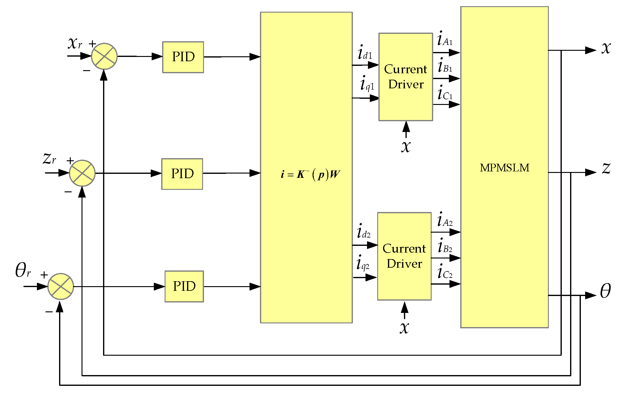
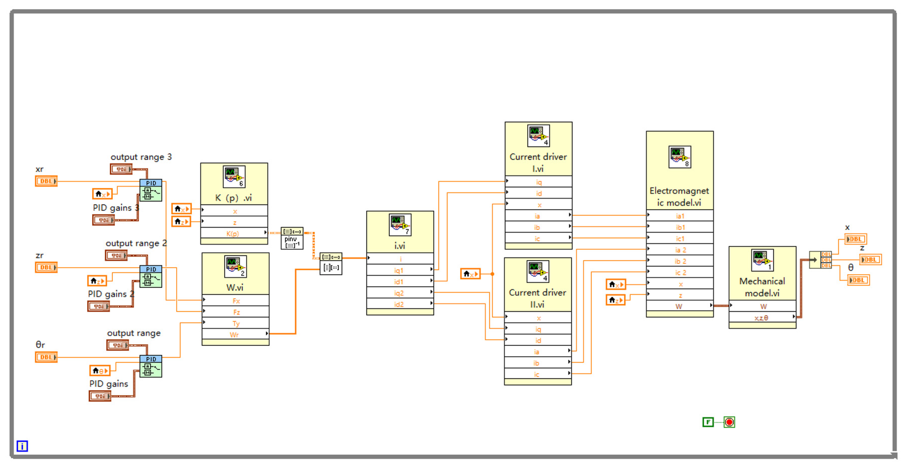
4.2. Structure of Control System
4.3. Position Closed-Loop Control
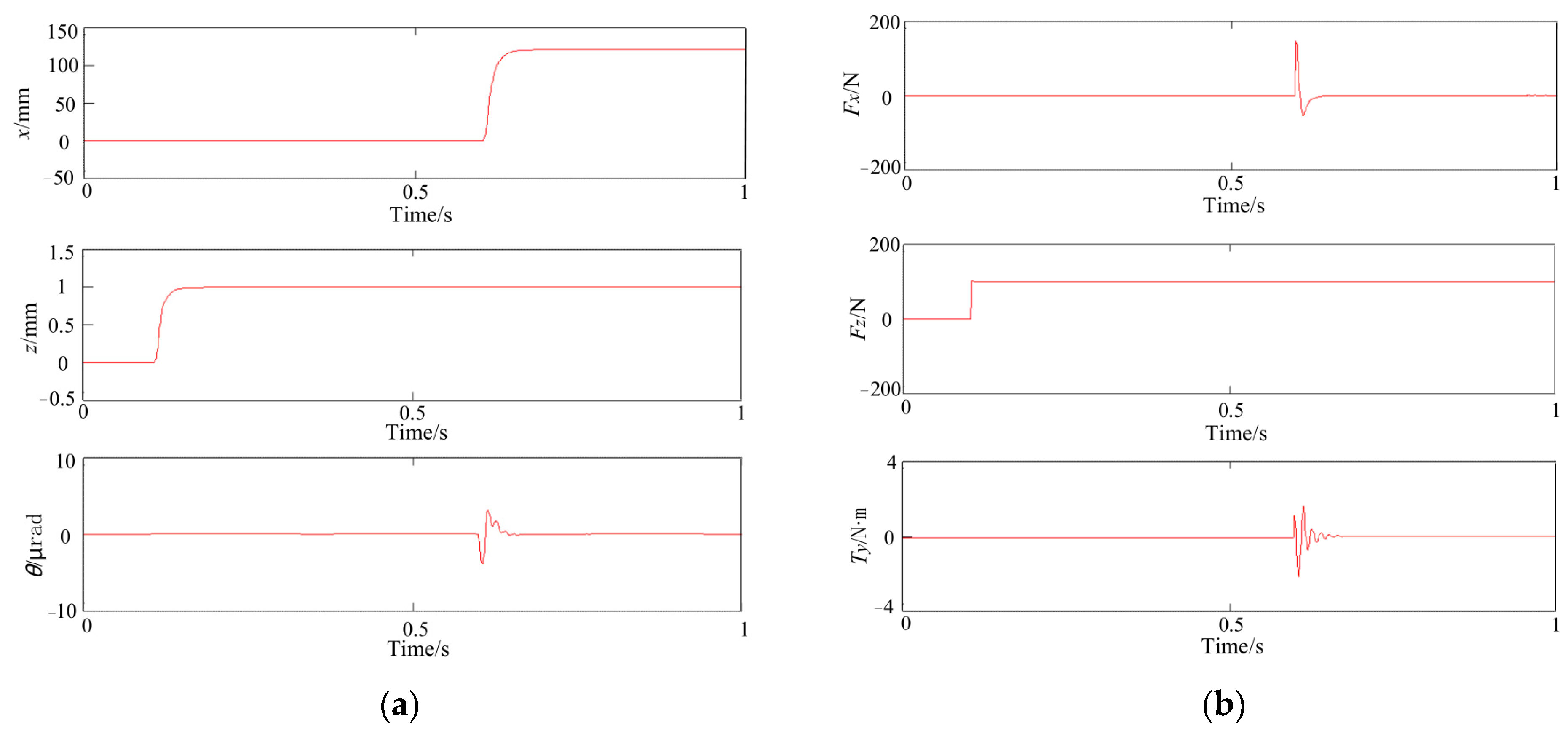
4.4. Result Analysis
5. Conclusions
Author Contributions
Funding
Data Availability Statement
Conflicts of Interest
References
- Lu, M.H.; Cao, R.W. Comparative investigation of high temperature superconducting linear flux-switching motor and high temperature superconducting linear switched reluctance motor for urban railway transit. IEEE Trans. Appl. Supercond. 2021, 31, 3600605. [Google Scholar] [CrossRef]
- Xu, L.; Sun, Z.M.; Zhao, W.X.; Liu, B.; Du, K.K.; Liu, G.H. Design and evaluation of linear primary permanent magnet vernier machines for urban railway transportation. IEEE Trans. Ind. Appl. 2023, 59, 1678–1688. [Google Scholar] [CrossRef]
- Liu, Z.H.; Cai, C.G.; Lv, Q.; Yang, M. Improved control of linear motors for broadband transducer calibration. IEEE Trans. Instrum. Meas. 2021, 70, 1004910. [Google Scholar] [CrossRef]
- Liu, Y.B.; Sun, W.C.; Buccella, C.; Cecati, C. Robust control of dual-linear-motor-driven gantry stage for coordinated contouring tasks based on feed velocity. IEEE Trans. Ind. Electron. 2023, 70, 6229–6238. [Google Scholar] [CrossRef]
- Deng, C.; Ye, C.Y.; Yang, J.T.; Sun, S.J.; Yu, D.Z. A novel permanent magnet linear motor for the application of electromagnetic launch system. IEEE Trans. Appl. Supercond. 2020, 30, 4902005. [Google Scholar] [CrossRef]
- Samimi, M.; Hassannia, A. Investigation of multi-layer secondary concept of an electromagnetic launcher. IEEE Trans. Energy Convers. 2022, 37, 921–926. [Google Scholar] [CrossRef]
- Cao, R.W.; Cheng, M.; Zhang, B.F. Speed control of complementary and modular linear flux-switching permanent-magnet motor. IEEE Trans. Ind. Electron. 2015, 62, 4056–4064. [Google Scholar] [CrossRef]
- Lu, Q.F.; Zhang, X.M.; Chen, Y.; Huang, X.Y.; Ye, Y.Y.; Zhu, Z.Q. Modeling and investigation of thermal characteristics of a water-cooled permanent-magnet linear motor. IEEE Trans. Ind. Appl. 2015, 51, 2086–2096. [Google Scholar] [CrossRef]
- Xi, J.S.; Dong, Z.G.; Liu, P.K.; Ding, H. Modeling and identification of iron-less PMLSM end effects for reducing ultra-low-velocity fluctuations of ultra-precision air bearing linear motion stage. Precis. Eng. 2017, 49, 92–103. [Google Scholar] [CrossRef]
- Mori, S.; Hoshino, T.; Obinata, G.; Ouchi, K. Air-bearing linear actuator for highly precise tracking. IEEE Trans. Magn. 2003, 39, 812–818. [Google Scholar] [CrossRef]
- Lv, G.; Zhang, Z.X.; Liu, Y.Q.; Zhou, T. Analysis of forces in linear synchronous motor with propulsion, levitation and guidance for high-speed maglev. IEEE J. Emerg. Sel. Top. Power Electron. 2022, 10, 2903–2911. [Google Scholar] [CrossRef]
- Lan, Y.P.; Li, J.; Zhang, F.G.; Zong, M. Fuzzy sliding mode control of magnetic levitation system of controllable excitation linear synchronous motor. IEEE Trans. Ind. Appl. 2020, 56, 5585–5592. [Google Scholar]
- Wang, H.L.; Li, J.; Qu, R.H.; Lai, J.Q.; Huang, H.L.; Liu, H.K. Study on high efficiency permanent magnet linear synchronous motor for maglev. IEEE Trans. Appl. Supercond. 2018, 28, 0601005. [Google Scholar] [CrossRef]
- Zhou, L.; Trumper, D.L. Magnetically levitated linear stage with linear bearingless slice hysteresis motors. IEEE/ASME Trans. Mechatron. 2021, 26, 1084–1094. [Google Scholar] [CrossRef]
- Teo, T.J.; Zhu, H.Y.; Pang, C.K. Modeling of a Two degrees-of-freedom moving magnet linear motor for magnetically levitated positioners. IEEE Trans. Magn. 2014, 50, 8300512. [Google Scholar] [CrossRef]
- Jansen, J.W.; van Lierop, C.M.M.; Lomonova, E.A.; Vandenput, A.J.A. Magnetically levitated planar actuator with moving magnets. IEEE Trans. Ind. Appl. 2008, 44, 1108–1115. [Google Scholar] [CrossRef]
- van Lierop, C.M.M.; Jansen, J.W.; Damen, A.A.H.; Lomonova, E.A.; van den Bosch, P.P.J.; Vandenput, A.J.A. Model-based commutation of a long-stroke magnetically levitated linear actuator. IEEE Trans. Ind. Appl. 2009, 45, 1982–1990. [Google Scholar] [CrossRef]
- Zhang, Y.M.; Ding, K.Z.; Du, S.S. Design study of a high loading superconducting magnetically levitated planar motor. IEEE Trans. Appl. Supercond. 2021, 31, 3601504. [Google Scholar] [CrossRef]
- Overboom, T.T.; Smeets, J.P.C.; Jansen, J.W.; Lomonova, E. Torque decomposition and control in an iron core linear permanent magnet motor. In Proceedings of the 2012 IEEE Energy Conversion Congress and Exposition (ECCE), Raleigh, NC, USA, 15–20 September 2012; pp. 2662–2669. [Google Scholar]
- van Lierop, C.M.M. Magnetically Levitated Planar Actuator with Moving Magnets: Dynamics, Commutation and Control Design. Ph.D. Thesis, Eindhoven University of Technology, Eindhoven, The Netherlands, November 2008. [Google Scholar]
- Xing, F.; Kou, B.Q.; Zhang, L.; Wang, T.C.; Zhang, C.N. Analysis and design of a maglev permanent magnet synchronous linear motor to reduce additional torque in dq current control. Energies 2017, 11, 556. [Google Scholar] [CrossRef]
- Kim, W.J. High-Precision Planar Magnetic Levitation. Ph.D. Thesis, Massachusetts Institute of Technology, Cambridge, MA, USA, June 1997. [Google Scholar]
- Teo, T.J.; Chen, I.M.; Yang, G.; Lin, W. Magnetic field modeling of a dual-magnet configuration. J. Appl. Phys. 2007, 102, 074924. [Google Scholar] [CrossRef]
- Zhu, H.Y.; Teo, T.J.; Pang, C.K. Design and modeling of a six-degree-of-freedom magnetically levitated positioner using square coils and 1-D Halbach arrays. IEEE Trans. Ind. Electron. 2017, 64, 440–450. [Google Scholar] [CrossRef]
- Jansen, J.W.; Lomonova, E.A.; Vandenput, A.J.A.; van Lierop, C.M.M. Analytical model of a magnetically levitated linear actuator. In Proceedings of the Fourtieth IAS Annual Meeting. Conference Record of the 2005 Industry Applications Conference, Hong Kong, China, 2–6 October 2005; pp. 2107–2113. [Google Scholar]
- Cao, J.C.; Deng, X.Q.; Li, D.; Jia, B. Electromagnetic analysis and optimization of high-speed maglev linear synchronous motor based on field-circuit coupling. CES Trans. Elect. Mach. Syst. 2022, 6, 118–123. [Google Scholar] [CrossRef]
- Jansen, J.W. Magnetically Levitated Planar Actuator with Moving Magnets: Electromechanical Analysis and Design. Ph.D. Thesis, Eindhoven University of Technology, Eindhoven, The Netherlands, November 2007. [Google Scholar]
- Zhang, S.G.; Niu, L.; Zhou, L.J.; Huang, J.T.; Hu, W.W.; Zhang, G.Q. Optimal matching design of length and width of rectangular ironless coils for magnetically levitated planar motors. IEEE Access 2019, 7, 185301–185309. [Google Scholar] [CrossRef]
- Liao, Z.M.; Yue, J.G.; Lin, G.B. Application research of HTS linear motor based on Halbach array in high speed maglev system. IEEE Trans. Appl. Supercond. 2021, 31, 3600707. [Google Scholar] [CrossRef]
- Shen, Y.M.; Lu, Q.F.; Li, Y.X. Design criterion and analysis of hybrid-excited vernier reluctance linear machine with slot Halbach PM arrays. IEEE Trans. Ind. Electron. 2023, 70, 5074–5084. [Google Scholar] [CrossRef]
- Qin, W.; Ma, Y.H.; Lv, G.; Wang, F.Y.; Zhao, J.D. New levitation scheme with traveling magnetic electromagnetic Halbach array for EDS maglev system. IEEE Trans. Magn. 2022, 58, 8300106. [Google Scholar] [CrossRef]


| Components | Materials |
|---|---|
| Coil | Copper |
| Permanent magnet | NdFe36 |
| Yoke plate | Steel_1010 |
| Parameters | Value | Unit |
|---|---|---|
| Pole pitch τ | 15 | mm |
| Air gap δ | 1 | mm |
| Winding size (lc × wc × hc) | 100 × 8 × 15 | mm |
| Major permanent magnet size (lm × w1 × hm) | 100 × 8.7 × 20 | mm |
| Auxiliary permanent magnet size (lm × w2 × hm) | 100 × 6.3 × 20 | mm |
| Controller | Kc | Ti | Td |
|---|---|---|---|
| x-axis controller | 112 | 0.032 | 0.00008 |
| z-axis controller | 120 | 0.036 | 0.000075 |
| θ-axis controller | 352 | 0.008 | 0.00001 |
| Parameters | Proposed Model (I) | Model in Figure 1 (II) | II/I |
|---|---|---|---|
| Positive direction θ | 3.25 μrad | 5.23 μrad | 1.61 |
| Negative direction θ | −3.89 μrad | −6.95 μrad | 1.79 |
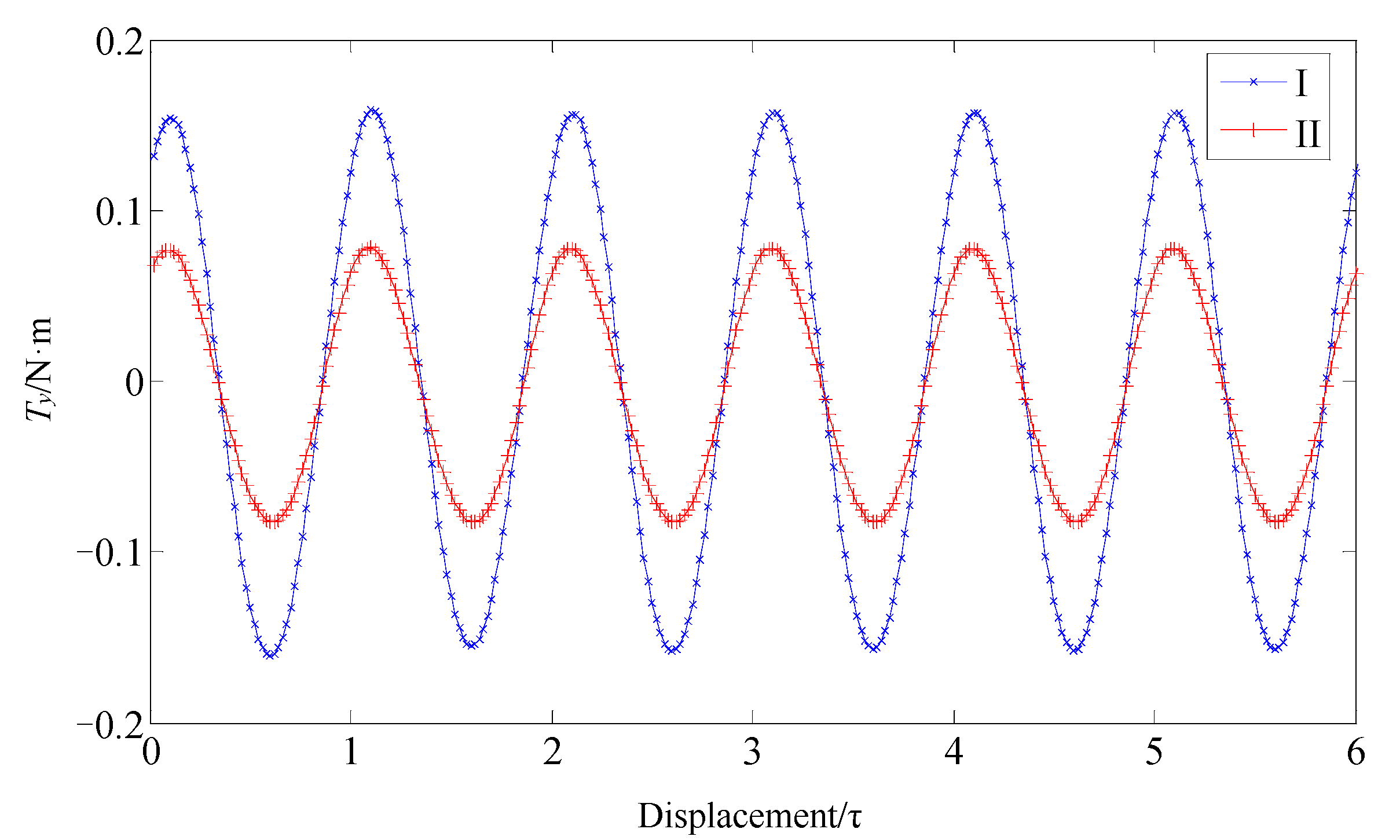
| Positive direction Ty | 1.62 N·m | 2.42 N·m | 1.49 |
| Negative direction Ty | −2.09 N·m | −2.85 N·m | 1.36 |
| Parameters | Proposed Model (I) | Model in Figure 1 (II) | II/I |
|---|---|---|---|
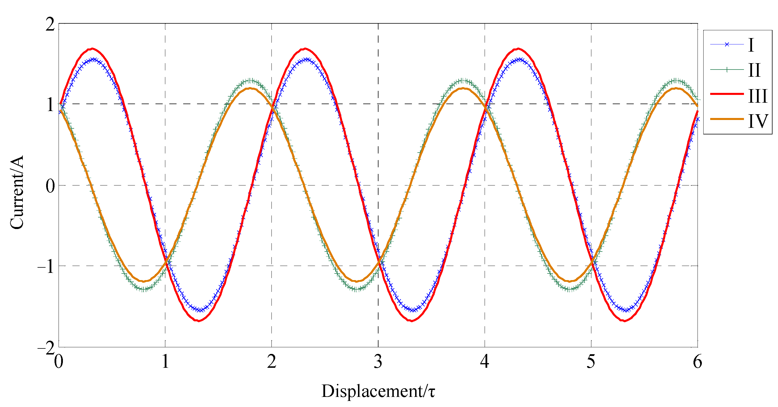
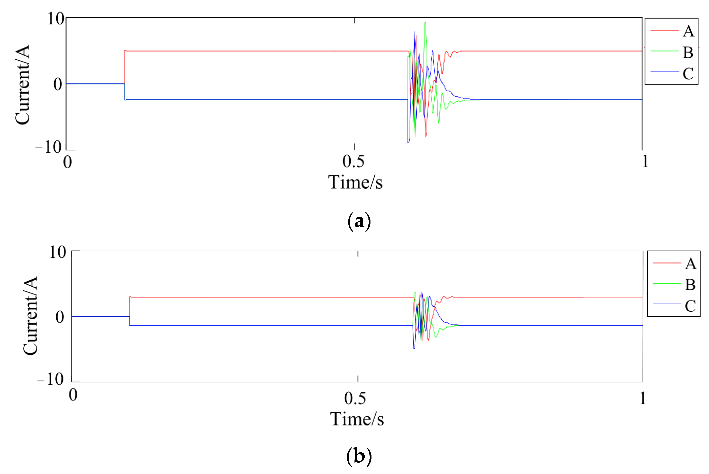
| |iAmax| | 3.55 A | 7.96 A | 2.24 |
| |iBmax| | 3.63 A | 9.26 A | 2.55 |
| |iCmax| | 4.85 A | 8.87 A | 1.83 |
Disclaimer/Publisher’s Note: The statements, opinions and data contained in all publications are solely those of the individual author(s) and contributor(s) and not of MDPI and/or the editor(s). MDPI and/or the editor(s) disclaim responsibility for any injury to people or property resulting from any ideas, methods, instructions or products referred to in the content. |
© 2023 by the authors. Licensee MDPI, Basel, Switzerland. This article is an open access article distributed under the terms and conditions of the Creative Commons Attribution (CC BY) license (https://creativecommons.org/licenses/by/4.0/).
Share and Cite
Xing, F.; Song, X.; Gao, Y.; Zhang, C. Toward Reducing Undesired Rotation Torque in Maglev Permanent Magnet Synchronous Linear Motor. Energies 2023, 16, 6066. https://doi.org/10.3390/en16166066
Xing F, Song X, Gao Y, Zhang C. Toward Reducing Undesired Rotation Torque in Maglev Permanent Magnet Synchronous Linear Motor. Energies. 2023; 16(16):6066. https://doi.org/10.3390/en16166066
Chicago/Turabian StyleXing, Feng, Xiaoyu Song, Yuge Gao, and Chaoning Zhang. 2023. "Toward Reducing Undesired Rotation Torque in Maglev Permanent Magnet Synchronous Linear Motor" Energies 16, no. 16: 6066. https://doi.org/10.3390/en16166066
APA StyleXing, F., Song, X., Gao, Y., & Zhang, C. (2023). Toward Reducing Undesired Rotation Torque in Maglev Permanent Magnet Synchronous Linear Motor. Energies, 16(16), 6066. https://doi.org/10.3390/en16166066