

Energy Storage Mix Optimization Based on Time Sequence Analysis Methodology for Surplus Renewable Energy Utilization


Abstract
:1. Introduction
2. Estimation of Surplus Renewable Energy in Future Carbon-Neutral Power Systems
2.1. Method of Surplus Renewable Energy Estimation
2.2. Method of Net Load Calculation
- NLt: Net Load per time slot (GW)
- GLt: Gross Load per time slot (GW)
- RGt: Renewable energy generation per time slot (GW)
- GLt: Gross Load per time slot (GW)
- Lt2018: Load historical data per time slot for 2018 (GW)
- Lpeak2018: Peak load historical data for 2018 (GW)
- Lpeak: Peak load forecast data for the analysis target year (GW)
- RGt: Renewable energy generation per time slot (GW)
- PVPt: PV generation pattern per time slot
- WPt: Wind generation pattern per time slot
- CapPV: PV generation capacity (GW)
- CapWind: Wind generation capacity (GW)
- PVGt: Solar power output per time slot (GW)
- PVGmax: Maximum solar power output (GW)
- WGt: Wind power output per time slot (GW)
- WGmax: Maximum wind power output (GW)
2.3. Method of Minimum Generation Constraint Calculation
- NGtCI_min: Minimum number of operating generators per time slot required to maintain the minimum inertia (units)
- CIt: Critical inertia; minimum inertia requirement per time slot (GWs)
- GCaverage: Average generation capacity (GW)
- ICaverage: Average generation inertia constant (sec)
- SGOtCI_min: Minimum generation constraint per time slot required to maintain the minimum inertia (GW)
- NGtCI_min: Minimum number of operating generators per time slot required to maintain the minimum inertia (units)
- GCaverage: Average generation capacity (GW)
- GOaveragemin: Average minimum level of generation output (%).
- NGtCI_min: Minimum number of operating generators per time slot required to maintain the operational reserve power (units)
- MSRmin: Minimum required operational reserve power (minimum spinning reserve) (GW)
- NLt: Net Load per time slot (GW)
- GCaverage: Average generator capacity (GW)
- RSRaverage: Average operational reserve power provision ratio per generator (%)
- SGOtSR_min: Minimum generation constraint per time slot required to maintain the operational reserve power (GW)
- NGtSR_min: Minimum number of operating generators per time slot required to maintain the operational reserve power (units)
- GCaverage: Average generator capacity (GW)
- GOaveragemin: Average minimum level of generation output (%)
- SGOtmin: Minimum generation constraint per time slot (GW)
- SGOtCI_min: Minimum generation constraint per time slot required to maintain the minimum inertia (GW)
- SGOtSR_min: Minimum generation constraint per time slot required to maintain the operational reserve power (GW)
2.4. Method of Surplus Renewable Energy Calculation
- SEt: Surplus energy per time slot (MW)
- NLt: Net Load per time slot (MW)
- MGt: Minimum generation constraint per time slot (MW)
3. Energy Storage Mix Optimization
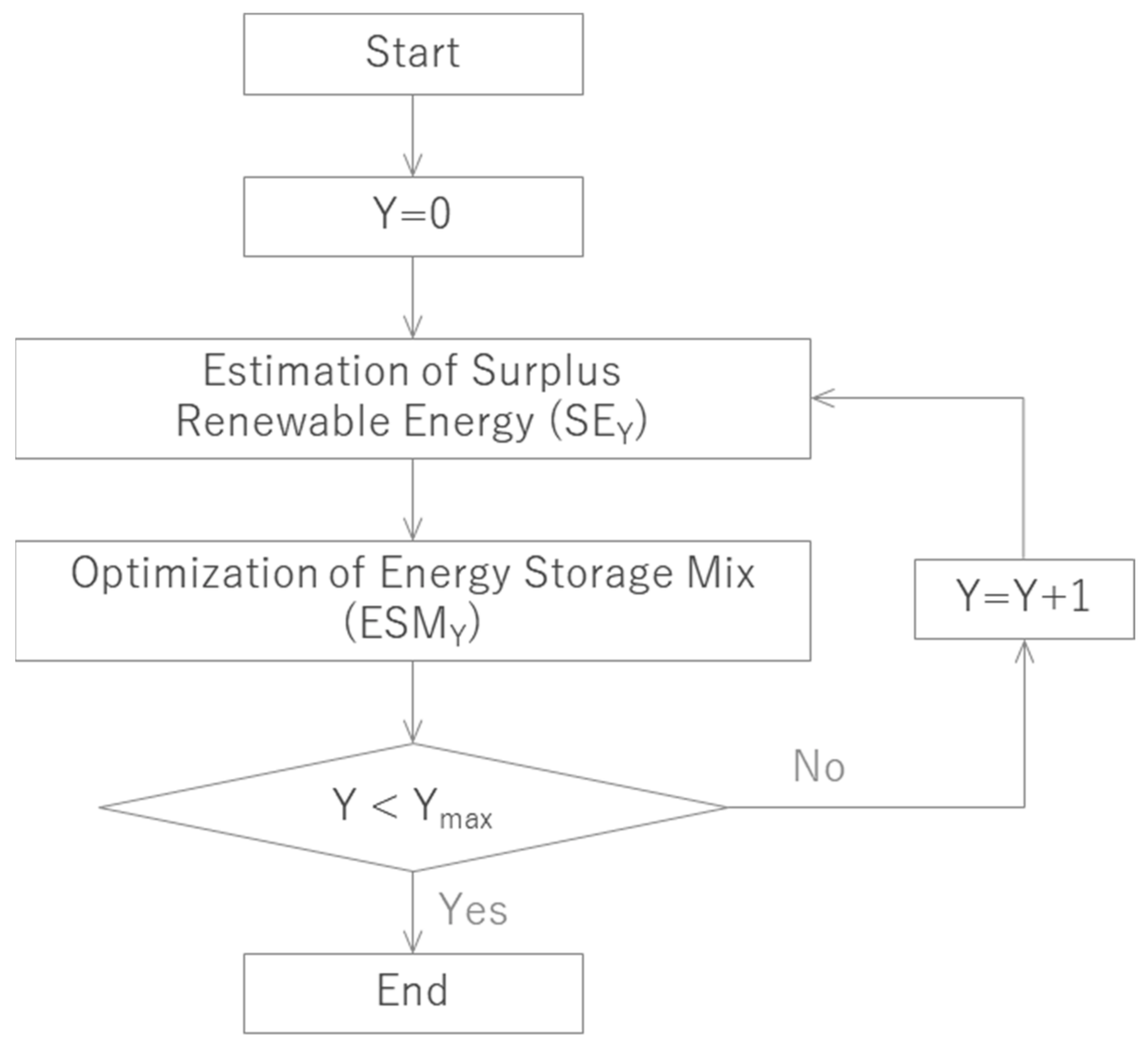
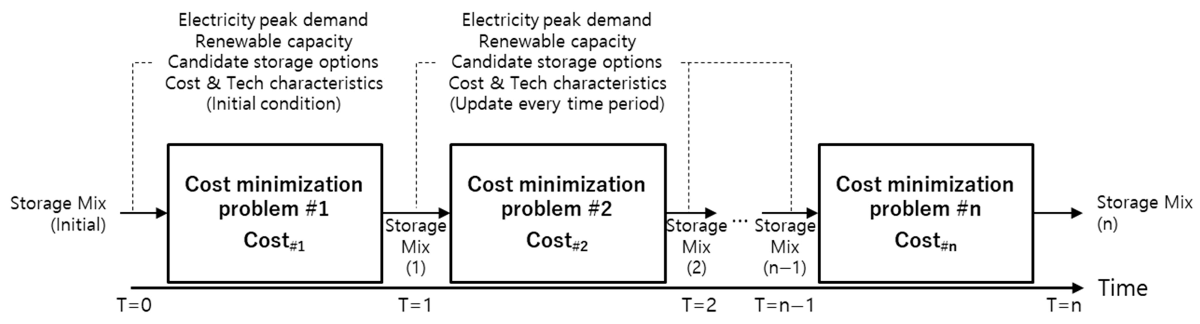
3.1. Time Sequence Analysis (TSA) Method
- COSTNPV: Net current value of the total cost over the entire period (hundred million KRW)
- COSTT: Cost per unit time (T) (hundred million KRW)
- r: Discount rate (%)
- ➀
- It efficiently resolves long-term equipment investment optimization problems. To resolve the entire long-term ESM optimization problem, the scale and complexity of the problem become enormous; thus, it is more efficient to divide the problem into set unit time slots and sequentially determine the optimal solution.
- ➁
- It considers the commercialization timing of target storage technology options. Currently, Li-ion batteries are the only energy storage technology that has been commercialized. The remaining technologies are currently under development, and the timing of their commercialization may vary based on various factors, such as the speed of technological development and economic feasibility. Therefore, the TSA method is applied to treat the commercialization timing of the target energy storage technology as an exogenous variable, not as an optimization target.
- ➂
- It considers changes in characteristics and costs of storage technologies for each step. In the long term, changes in characteristics and costs of storage technologies can occur owing to technological development and environmental changes. The TSA method is used to appropriately apply these changes for each step and to optimize the entire period.
3.2. Formulation of the Optimization Problem for Each Period
- COSTY: Total cost in year Y (hundred million KRW)
- ICY: Investment cost incurred to install new ESSs in year Y (hundred million KRW)
- RCY: Replacement and maintenance costs for the existing ESSs in year Y (hundred million KRW)
- LCY: Charging–discharging loss cost in year Y (hundred million KRW)
- ICY: Investment cost incurred to install new ESSs in year Y (hundred million KRW)
- RCY: Replacement and maintenance costs for the existing ESSs in year Y (hundred million KRW)
- LCY: Charging–discharging loss cost in year Y (hundred million KRW)
- CAPI,newpower: New power (PCS) equipment capacity for the I-th technology in the analysis year (MW)
- PIpower: Installation cost for new power (PCS) equipment for the I-th technology (hundred million KRW/MW)
- PIenergy: Installation unit cost for new energy (cell) equipment for the I-th technology (hundred million KRW/MWh)
- CAPI,Ypower: Power (PCS) equipment capacity for the I-th technology in year Y (MW)
- CAPI,Yenergy: Energy (cell) equipment capacity for the I-th technology in year Y (MWh)
- NCI,Y: Number of charging and discharging cycles for the I-th technology in year Y (Cycles)
- LTIpower: Lifespan of power (PCS) equipment for the I-th technology (Cycles)
- LTIenergy: Lifespan of energy (cell) equipment for the I-th technology (Cycles)
- μI: Charging and discharging loss rates for the I-th technology (%)
- PYelectricity: Price of electricity in year Y (KRW/kWh)
- CAPI,Ypower: Power (PCS) equipment capacity for the I-th technology in year Y (MW)
- CAPI,newpower: New power (PCS) equipment capacity for the I-th technology in the analysis year (MW)
- CAPI,Yenergy: Energy (cell) equipment capacity for the I-th technology in year Y (MWh)
- CAPI,newenergy: New power (PCS) equipment capacity for the I-th technology in the analysis year (MW)
- CAPYpower_req: Required power (PCS) equipment capacity in the analysis year (MW)
- CAPYenergy_req: Required energy (cell) equipment capacity in the analysis year (MWh)
- CAPI,newpower: New power (PCS) equipment capacity for the I-th technology in the analysis year (MW)
- CAPI,newenergy: New power (PCS) equipment capacity for the I-th technology in the analysis year (MW)
- CAPI,ypower_max: Maximum installation capacity of new power (PCS) equipment for the I-th technology (MW)
- CAPI,yenergy_max: Maximum installation capacity of new energy (cell) equipment for the I-th technology (MWh)
4. Case Study
4.1. Estimation of Surplus Renewable Energy
4.1.1. Preconditions and Input Data
- (1)
- Comparative analysis scenarios:
- (2)
- Electricity demand: The pattern of the gross electricity demand by time slot was normalized using the power demand pattern of 2018 when the proportion of renewable generation was less than 2%. The peak demand as shown in Table 1 for each year was obtained from the forecasts in South Korea’s 10th Basic Plan for Long-Term Electricity Supply and Demand and the 2050 Carbon-Neutrality Scenario [1,2,3].
- (3)
- Renewable generation: Solar and wind power were considered for renewable generation. The generation pattern by time slot was created using the actual generation output data from 2021. We created generation output patterns by time slot for each month to consider the characteristics of the renewable generation output by season. The capacity of the renewable energy generation equipment as shown in Table 2 was obtained from South Korea’s 10th Basic Plan for Long-Term Electricity Supply and Demand and the 2050 Carbon-Neutrality Scenario [1,2,3].
- (4)
- Critical inertia requirement: Although studies on the characteristics of the South Korean power system are yet to be conducted for critical inertia, we used the critical inertia level of 320 GW, as suggested in the 10th Basic Plan for Long-Term Electricity Supply and Demand, considering the frequency stability. The critical inertia suitable for the South Korean power system must be determined in future studies.
- (5)
- Minimum reserve power requirement: The minimum reserve power requirement can vary depending on changes in the proportion of renewable energy in the future; however, we used 1.7 GW, which is the sum of the frequency control and primary reserve power, as the minimum reserve power requirement based on the current reserve power standard. The Power Pool Rule (Grid Code) of the Korean power system divides the operational reserve power into four categories. The minimum requirement for securing the total reserve power is 4.5 GW (including 700 MW for frequency control, 1000 MW for primary reserve, 1400 MW for secondary reserve, and 1400 MW for alternative reserve). Among them, the minimum reserve power requirement was considered as 1.7 GW, which is the sum of the frequency control and primary reserve and is a spinning reserve [18].
- (6)
- Other matters: For calculating surplus energy, 1.0 GW was used as the equipment capacity of a standard thermal power generator, and the inertia constant was set to 5 s. In addition, the minimum stable output level of the generator was considered as 80% (nuclear power plant), 70% (coal-fired power plant), and 40% (gas-turbine power plant) of the rated capacity.
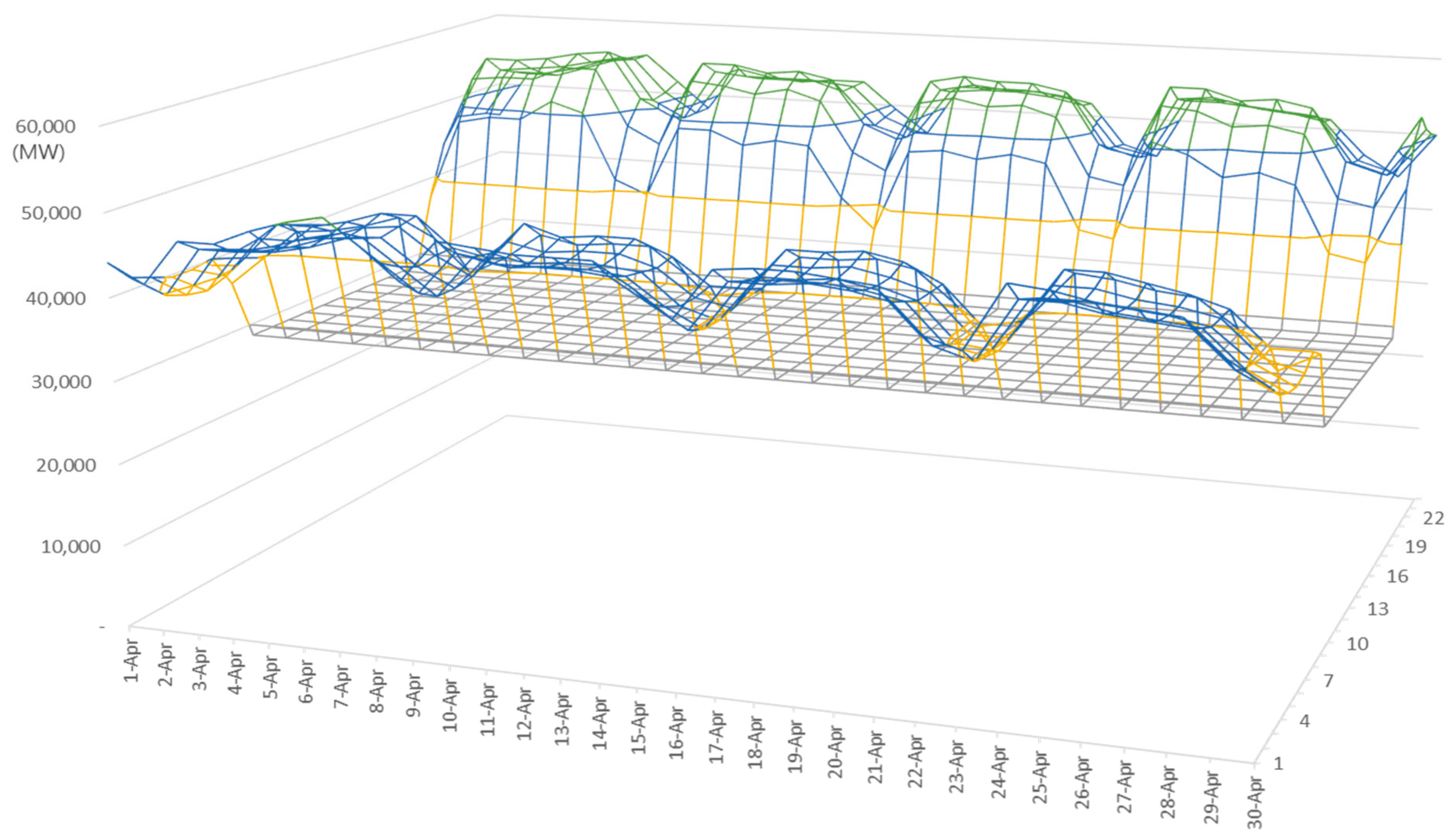
4.1.2. Calculation of Net Load
4.1.3. Minimum Generation Output Constraint
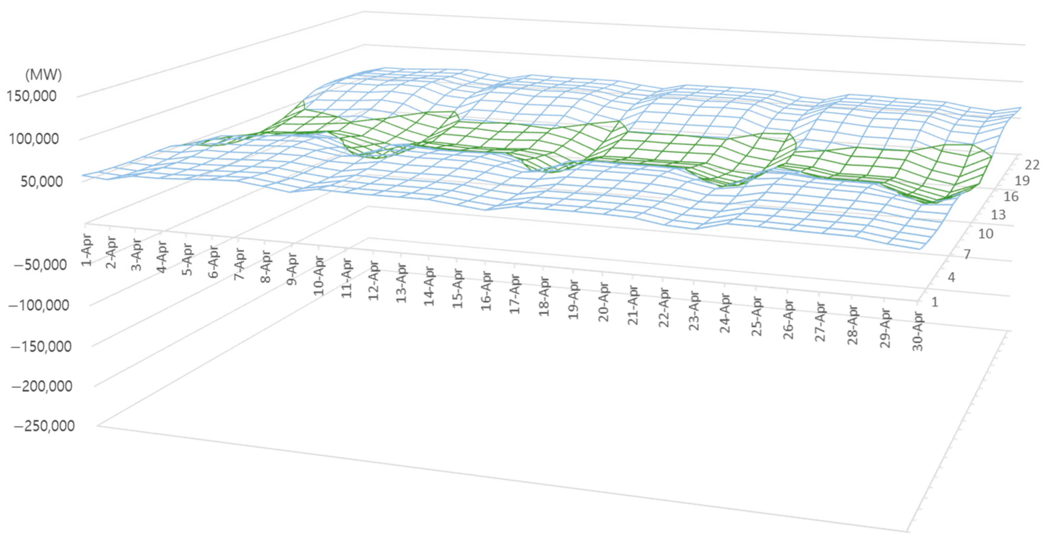
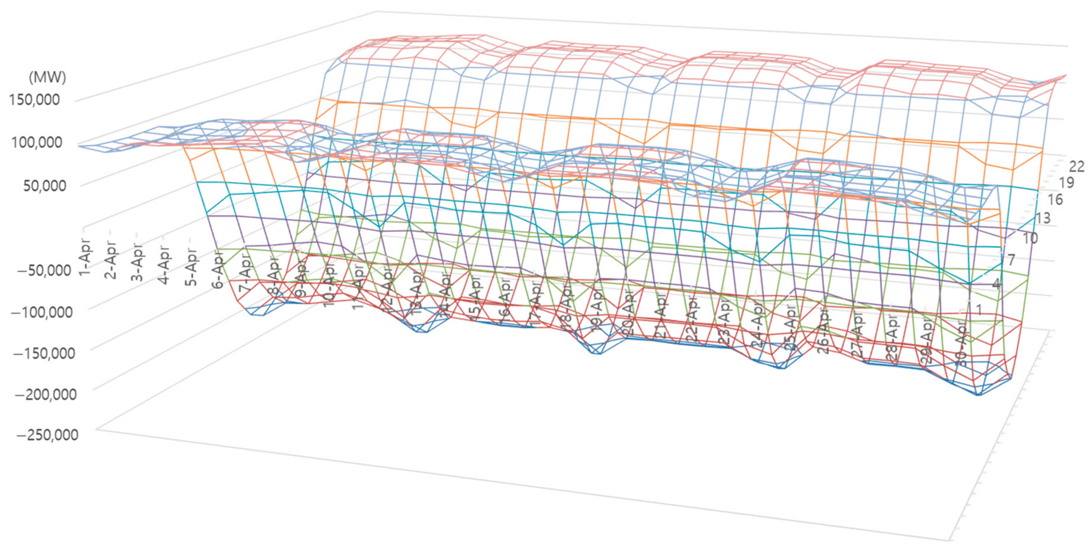
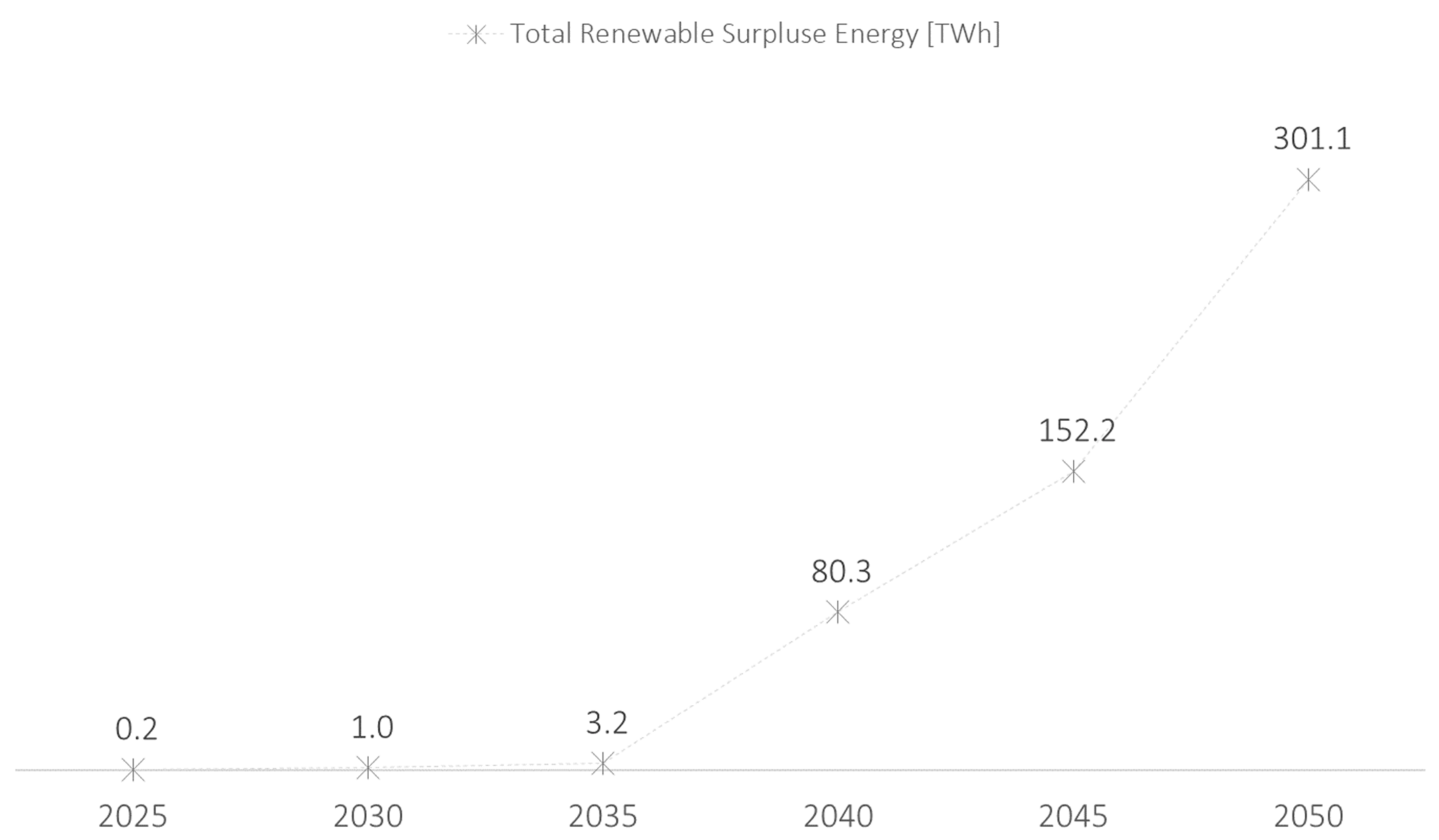
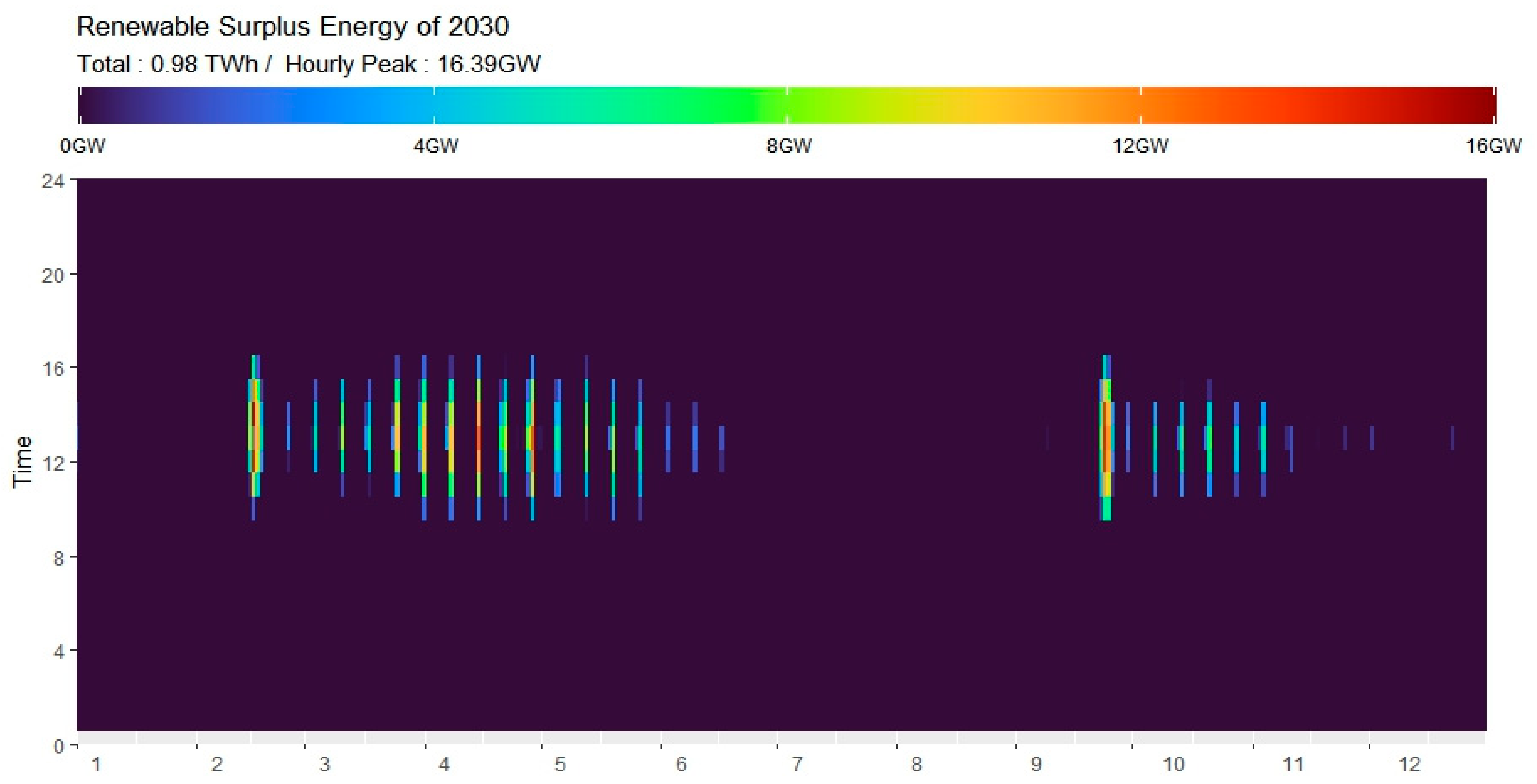
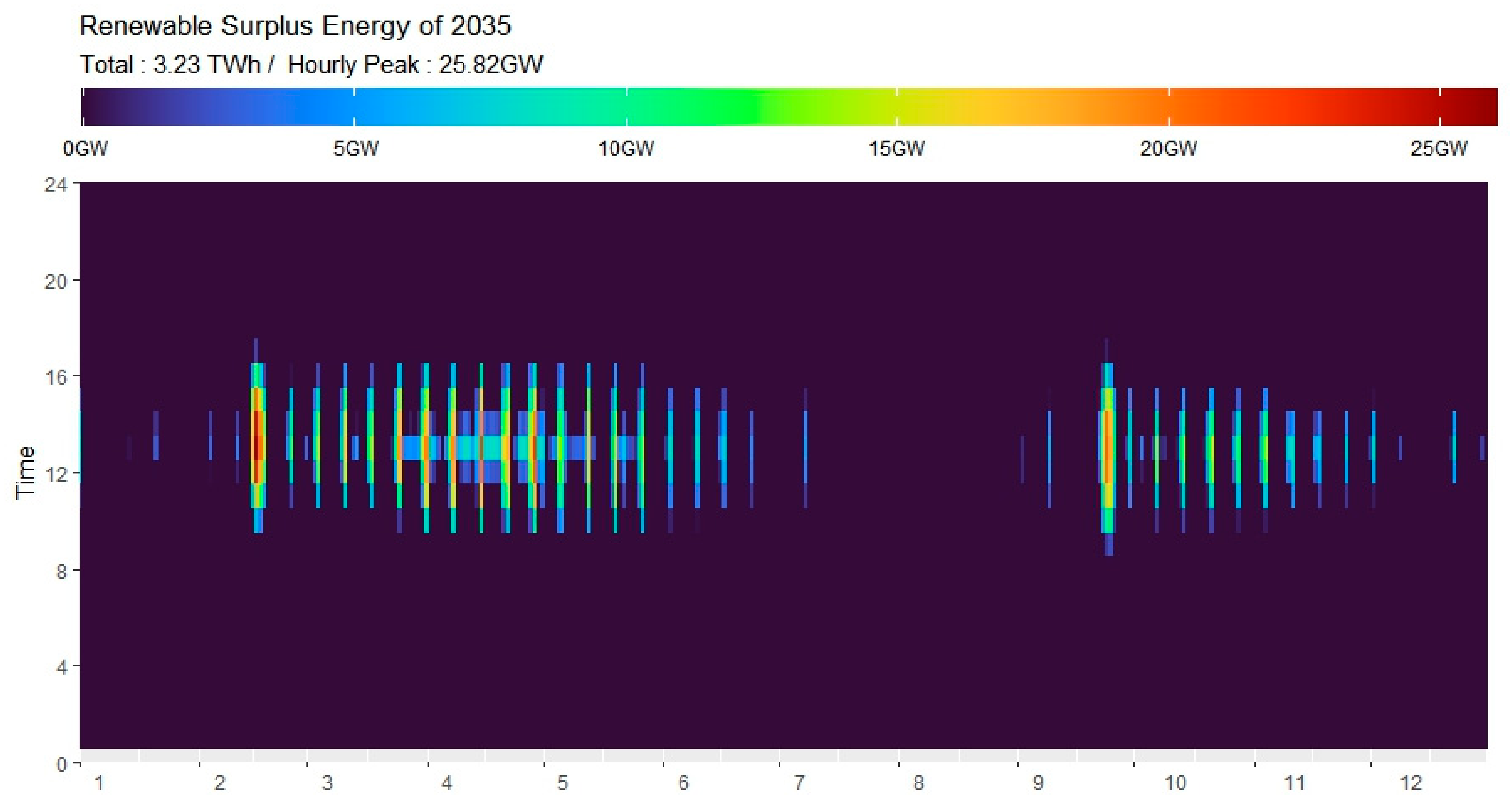
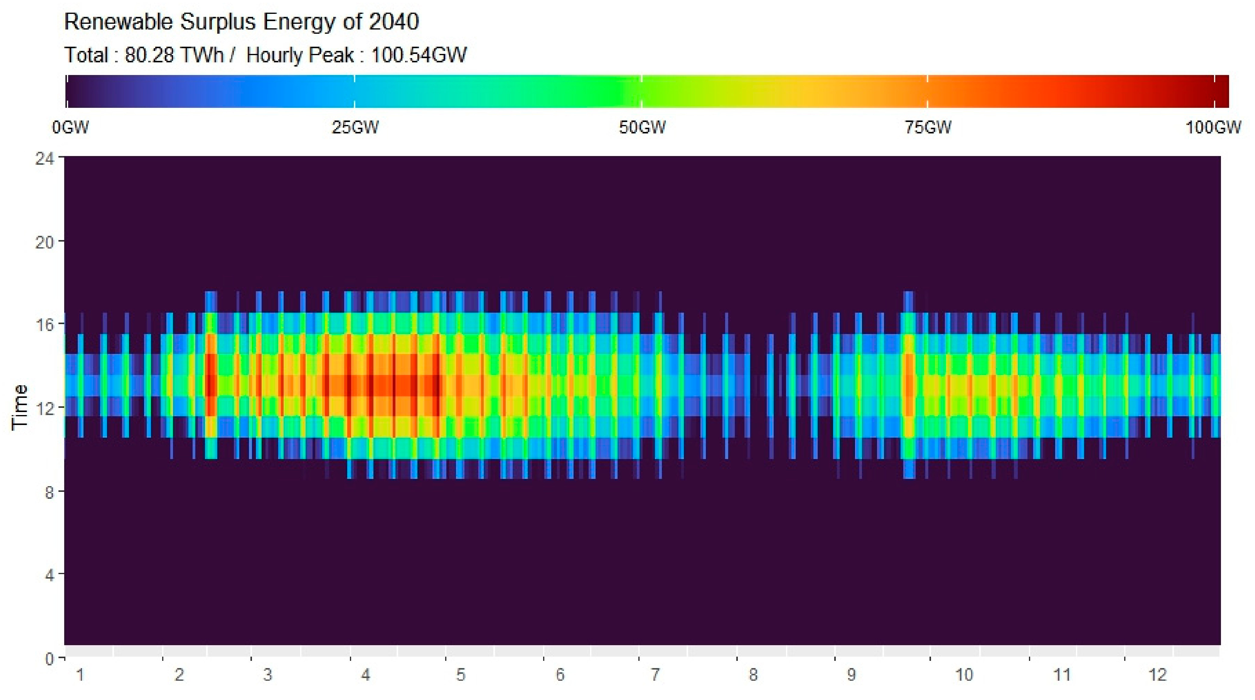
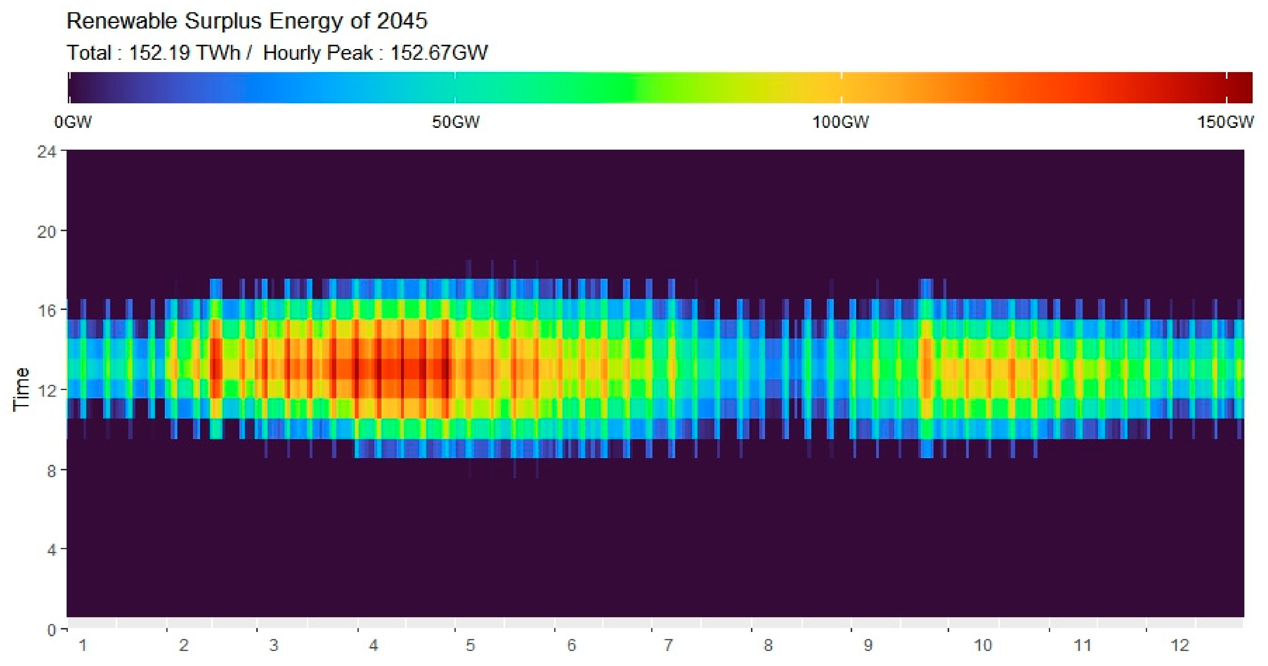
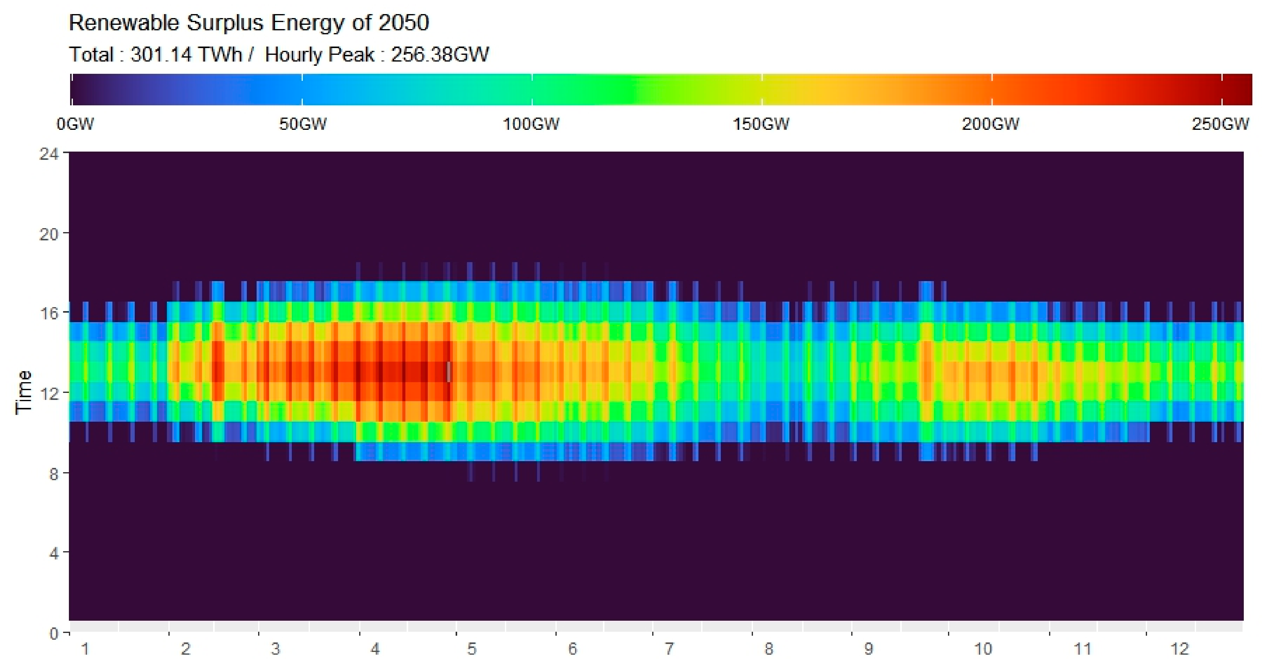
4.1.4. Estimation of Surplus Renewable Energy
- ➀
- It begins after 2030 and sharply increases from 2040.
- ➁
- Before 2035, it occurs only on holidays, when power demand is low; however, after 2040, it also occurs on weekdays.
- ➂
- Surplus renewable energy has a high concentration during daytime hours in spring and autumn, when solar generation increases, and power demand is low.
4.1.5. Energy Storage Capacity Requirement
4.2. Types and Characteristics of Energy Storage Technologies
4.3. Energy Storage Mix Optimization (2023–2050)
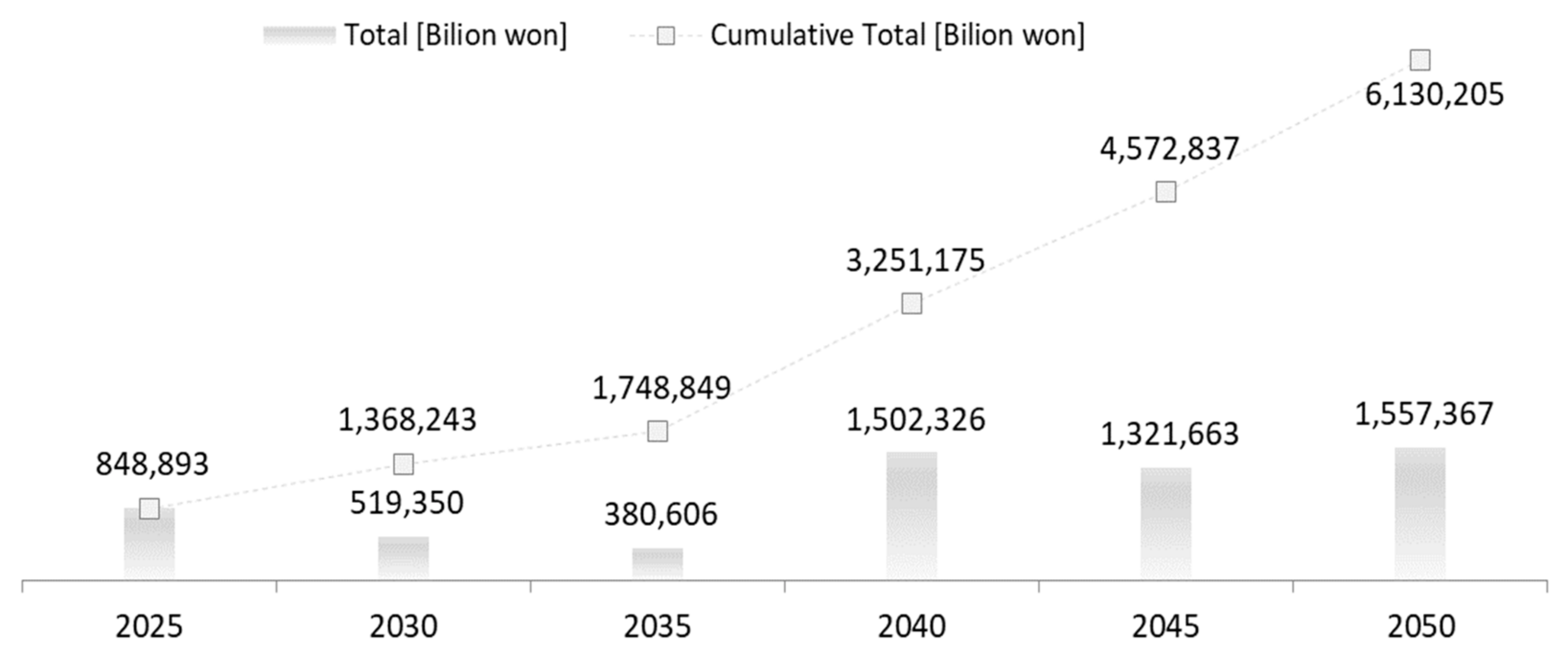
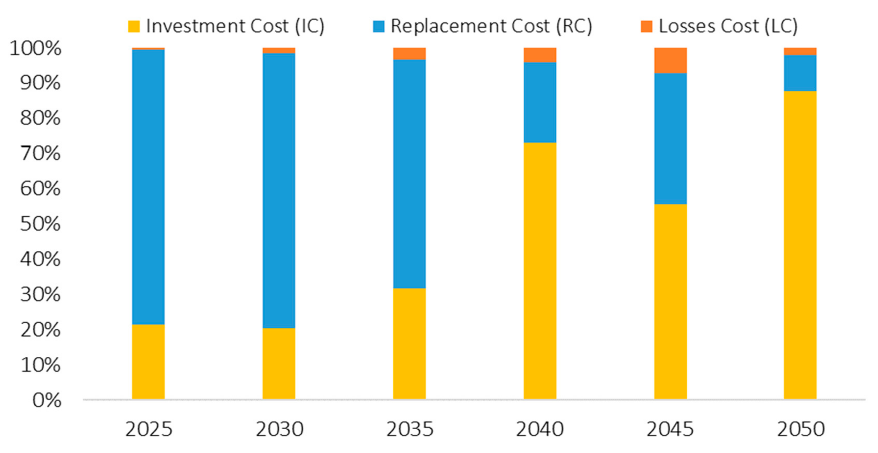
4.3.1. ESM Analysis Results Based on TSA
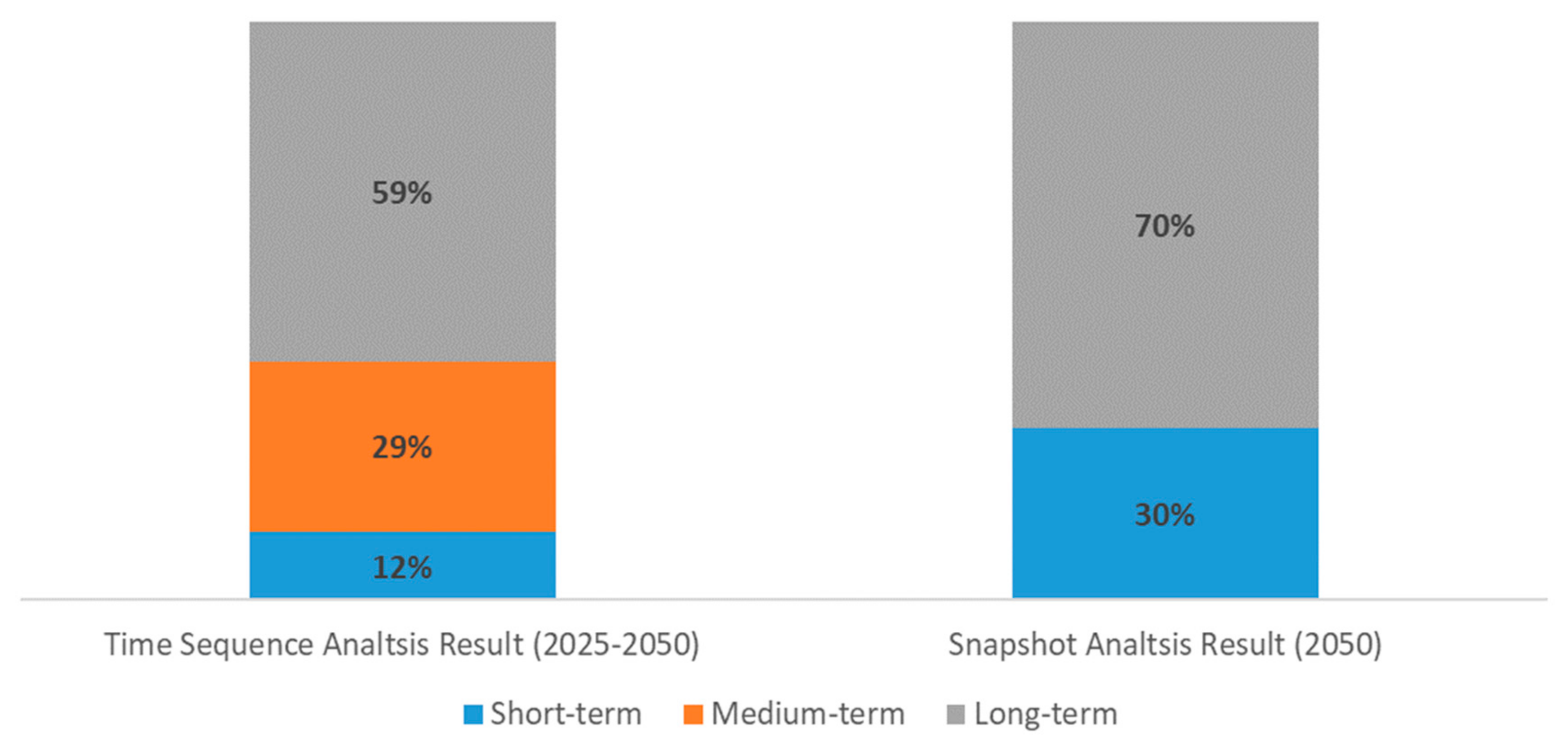
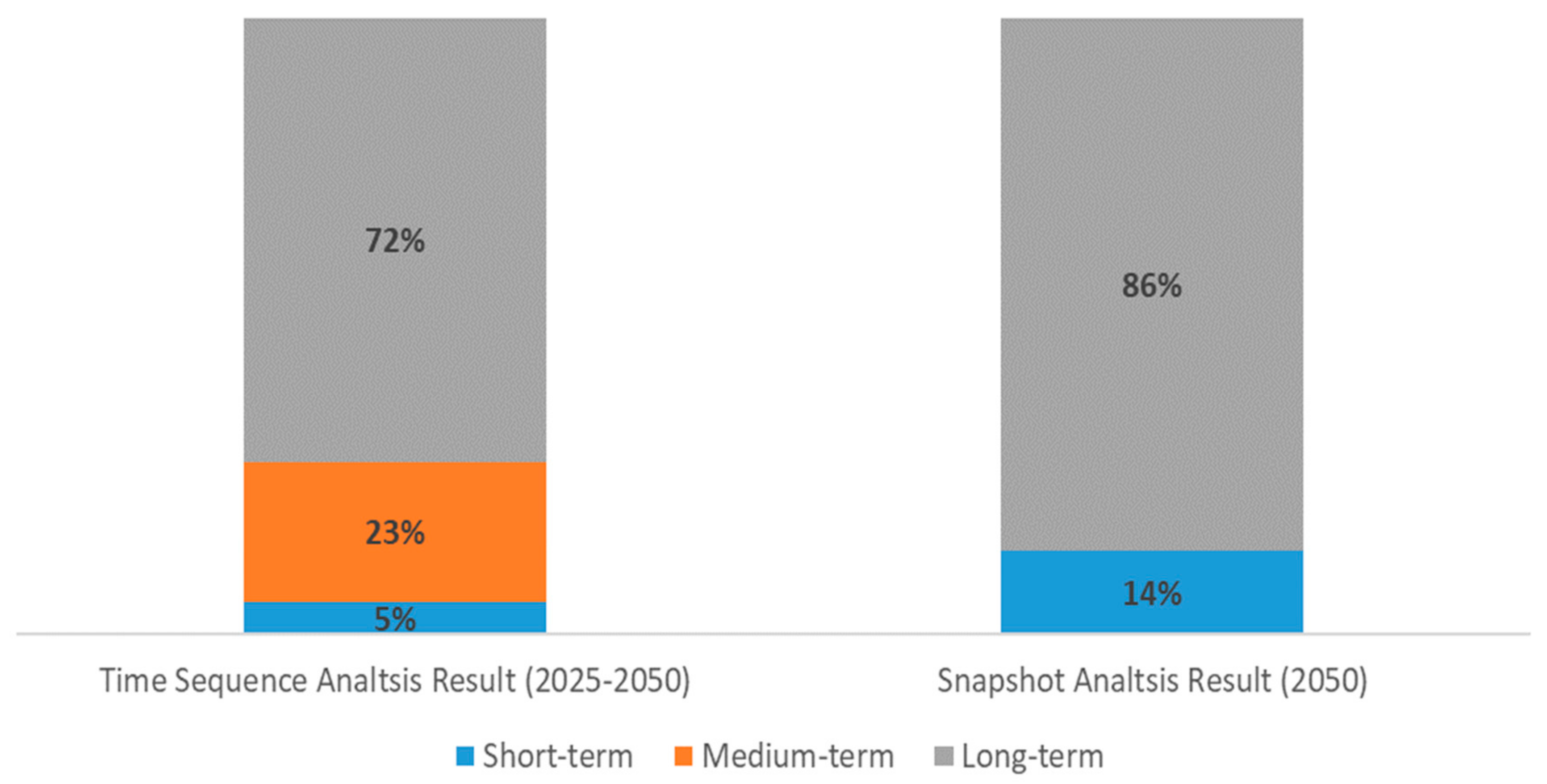
4.3.2. ESM Analysis Results and Comparison Based on Single-Year (2050) Optimization
5. Conclusions
Author Contributions
Funding
Data Availability Statement
Acknowledgments
Conflicts of Interest
References
- Government of the Republic of Korea. 2050 Carbon Neutral Scenario; Government of the Republic of Korea: Seoul, Republic of Korea, 2021.
- Ministry of Trade, Industry and Energy. The 10th Basic Plan for Electricity Supply and Demand; Ministry of Trade, Industry and Energy: Sejong City, Republic of Korea, 2023.
- Government of the Republic of Korea. National Carbon Neutrality and Green Growth Basic Plan; Government of the Republic of Korea: Seoul, Republic of Korea, 2023.
- Shi, Z.; Wang, W.; Huang, Y.; Li, P.; Dong, L. Simultaneous optimization of renewable energy and energy storage capacity with the hierarchical control. CSEE J. Power Energy Syst. 2020, 8, 95–104. [Google Scholar]
- Bian, B.P.; Du, Z.; Hao, C.; Wu, H.; Yan, L.; Hou, Z.; Chen, Y. Model and Method of Capacity Planning of Energy Storage Capacity for Integrated Energy Station. In Proceedings of the 2022 4th Asia Energy and Electrical Engineering Symposium (AEEES), Chengdu, China, 25–28 March 2022; IEEE: New York, NY, USA, 2022; pp. 410–415. [Google Scholar]
- Guo, Z.; Wei, W.; Chen, L.; Dong, Z.Y.; Mei, S. Impact of energy storage on renewable energy utilization: A geometric description. IEEE Trans. Sustain. Energy 2020, 12, 874–885. [Google Scholar] [CrossRef]
- Cao, X.; Cao, T.; Gao, F.; Guan, X. Risk-averse storage planning for improving RES hosting capacity under uncertain siting choices. IEEE Trans. Sustain. Energy 2021, 12, 1984–1995. [Google Scholar] [CrossRef]
- Salman, U.T.; Al-Ismail, F.S.; Khalid, M. Optimal sizing of battery energy storage for grid-connected and isolated wind-penetrated microgrid. IEEE Access 2020, 8, 91129–91138. [Google Scholar] [CrossRef]
- Geng, S.; Vrakopoulou, M.; Hiskens, I.A. Optimal capacity design and operation of energy hub systems. Proc. IEEE 2020, 108, 1475–1495. [Google Scholar] [CrossRef]
- Yao, M.; Cai, X. Energy storage sizing optimization for large-scale PV power plant. IEEE Access 2021, 9, 75599–75607. [Google Scholar] [CrossRef]
- Xie, P.; Cai, Z.; Liu, P.; Li, X.; Zhang, Y.; Xu, D. Microgrid system energy storage capacity optimization considering multiple time scale uncertainty coupling. IEEE Trans. Smart Grid 2018, 10, 5234–5245. [Google Scholar] [CrossRef]
- Yang, Y.; Bremner, S.; Menictas, C.; Kay, M. Battery energy storage system size determination in renewable energy systems: A review. Renew. Sustain. Energy Rev. 2018, 91, 109–125. [Google Scholar] [CrossRef]
- Sufyan, M.; Rahim, N.A.; Aman, M.M.; Tan, C.K.; Raihan, S.R.S. Sizing and applications of battery energy storage technologies in smart grid system: A review. J. Renew. Sustain. Energy 2019, 11, 014105. [Google Scholar] [CrossRef]
- Hannan, M.A.; Wali, S.B.; Ker, P.J.; Abd Rahman, M.S.; Mansor, M.; Ramachandaramurthy, V.K.; Dong, Z.Y. Battery energy-storage system: A review of technologies, optimization objectives, constraints, approaches, and outstanding issues. J. Energy Storage 2021, 42, 103023. [Google Scholar] [CrossRef]
- Alsaidan, I.; Khodaei, A.; Gao, W. A comprehensive battery energy storage optimal sizing model for microgrid applications. IEEE Trans. Power Syst. 2017, 33, 3968–3980. [Google Scholar] [CrossRef]
- Andrijanovits, A.; Hoimoja, H.; Vinnikov, D. Comparative review of long-term energy storage technologies for renewable energy systems. Elektron. Ir Elektrotech. 2012, 118, 21–26. [Google Scholar] [CrossRef]
- Haas, J.; Cebulla, F.; Nowak, W.; Rahmann, C.; Palma-Behnke, R. A multi-service approach for planning the optimal mix of energy storage technologies in a fully-renewable power supply. Energy Convers. Manag. 2018, 178, 355–368. [Google Scholar] [CrossRef]
- Korea Power eXchange (KPX). Power Pool Rule. Available online: https://marketrule.kpx.or.kr/lmxsrv/main/main.do (accessed on 14 August 2023).
- Spataru, C.; Kok, Y.C.; Barrett, M.; Sweetnam, T. Techno-economic assessment for optimal energy storage mix. Energy Procedia 2015, 83, 515–524. [Google Scholar] [CrossRef]
- Lund, H.; Münster, E. Management of surplus electricity-production from a fluctuating renewable-energy source. Appl. Energy 2003, 76, 65–74. [Google Scholar] [CrossRef]
- Bradbury, K. Energy Storage Technology Review; Duke University: Durham, NC, USA, 2010; pp. 1–34. [Google Scholar]
- Schmidt, O.; Hawkes, A.; Gambhir, A.; Staffell, I. The future cost of electrical energy storage based on experience rates. Nat. Energy 2017, 2, 1–8. [Google Scholar] [CrossRef]
- Guney, M.S.; Tepe, Y. Classification and assessment of energy storage systems. Renew. Sustain. Energy Rev. 2017, 75, 1187–1197. [Google Scholar] [CrossRef]


| Year | 2025 | 2030 | 2035 | 2040 | 2045 | 2050 |
|---|---|---|---|---|---|---|
| Peak Demand (GW) | 102.5 | 109.3 | 116.2 | 147.8 | 168.9 | 211.0 |
| Year | 2025 | 2030 | 2035 | 2040 | 2045 | 2050 |
|---|---|---|---|---|---|---|
| Renewable Generation Capacity (GW) | 34.7 | 65.8 | 94.6 | 261.5 | 372.7 | 595.3 |
| Year | Gross Load (MW) | Net Load (MW) | ||||
|---|---|---|---|---|---|---|
| Max | Min | Average | Max | Min | Average | |
| 2025 | 102,484 | 45,301 | 71,457 | 96,986 | 29,880 | 65,889 |
| 2030 | 109,300 | 48,314 | 76,210 | 101,467 | 20,521 | 64,507 |
| 2035 | 116,158 | 51,345 | 80,992 | 106,416 | 10,728 | 63,792 |
| 2040 | 147,772 | 65,320 | 103,035 | 132,125 | −66,295 | 70,155 |
| 2045 | 168,848 | 74,636 | 117,730 | 149,939 | −120,144 | 81,998 |
| 2050 | 211,000 | 93,268 | 147,121 | 186,193 | −227,842 | 104,369 |
| Year | Minimum Generation Output Constraint (MW) | ||
|---|---|---|---|
| Max | Min | Average | |
| 2025 | 59,018 | 38,542 | 42,182 |
| 2030 | 59,406 | 36,913 | 40,275 |
| 2035 | 61,676 | 36,548 | 40,120 |
| 2040 | 71,701 | 34,245 | 41,766 |
| 2045 | 76,739 | 32,525 | 42,688 |
| 2050 | 83,816 | 28,533 | 42,832 |
| Short Term | Medium Term | Long Term | |
|---|---|---|---|
| Rated output discharging duration (h) | 3 | 5 | 8 |
| Unit capacity (PCS/CELL) | 100 MW/300 MWh | 300 MW/1500 MWh | 500 MW/4000 MWh |
| Designed lifespan (PCS/CELL) | 1000/400 Cycles | 1000/2000 Cycles | 1000/5000 Cycles |
| Charging and discharging efficiency (%) | 90 | 50 | 40 |
| Year of Commercialization | Already commercialized | 2030 | 2035 |
| 2025 | 2030 | 2035 | 2040 | 2045 | 2050 | |
|---|---|---|---|---|---|---|
| Short term (PCS/CELL) | 1.00/4.00 | 0.99/3.92 | 0.98/3.84 | 0.97/3.76 | 0.96/3.69 | 0.95/3.62 |
| Medium term (PCS/CELL) | - | 0.99/3.00 | 0.98/2.85 | 0.97/2.71 | 0.96/2.57 | 0.95/2.44 |
| Long term (PCS/CELL) | - | - | 0.98/2.00 | 0.97/1.84 | 0.96/1.69 | 0.95/1.56 |
| 2025 | 2030 | 2035 | 2040 | 2045 | 2050 | |
|---|---|---|---|---|---|---|
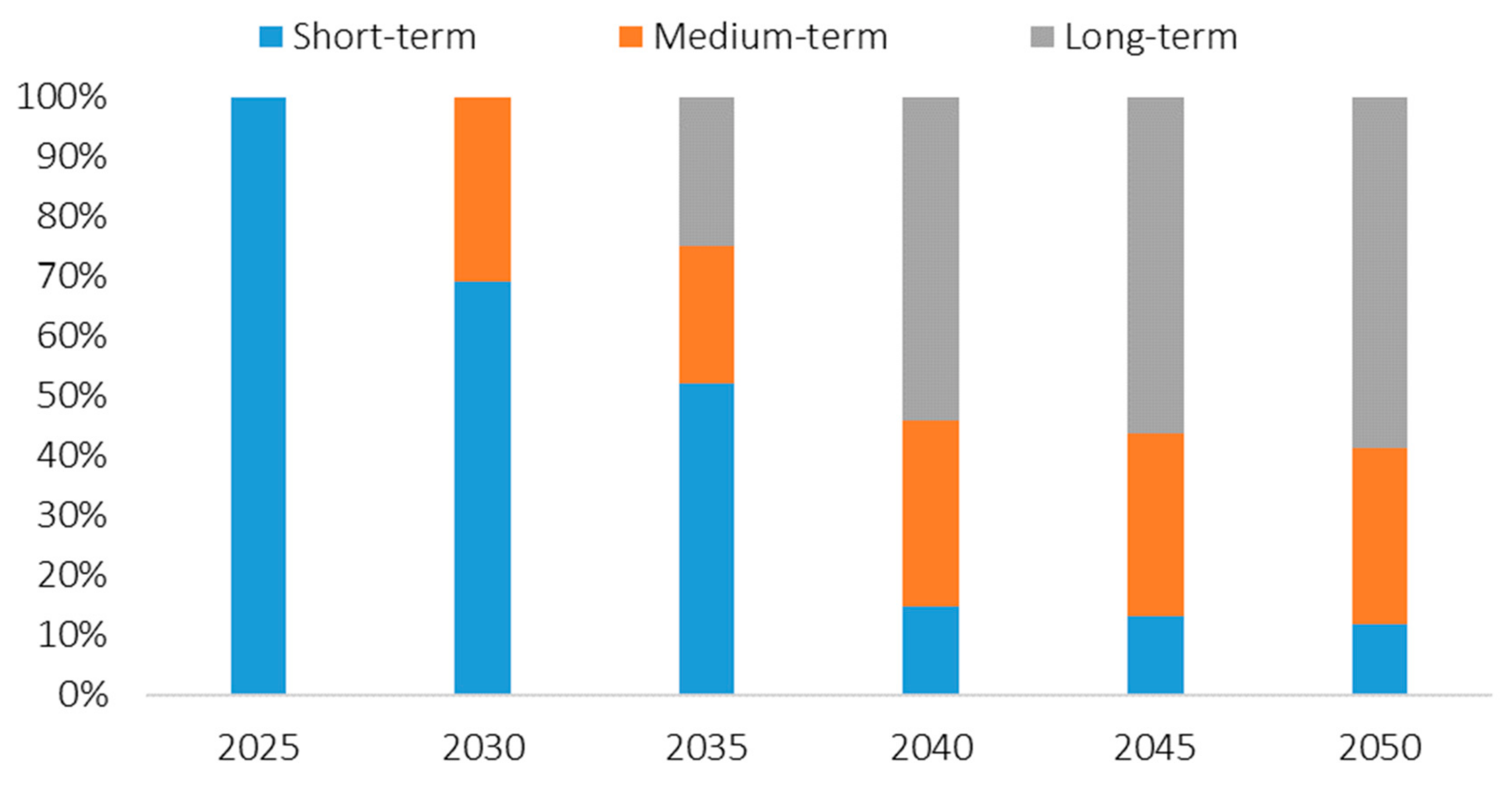
| Short term (GW) | 14.9 (100%) | 14.9 (69.2%) | 14.9 (52.1%) | 14.9 (14.9%) | 20.3 (13.3%) | 30.2 (11.8%) |
| Medium term (GW) | - | 6.6 (30.8%) | 6.6 (23.1%) | 31.3 (31.2%) | 46.7 (30.6%) | 75.6 (29.5%) |
| Long term (GW) | - | - | 7.1 (24.8%) | 54.2 (54.0%) | 85.7 (56.1%) | 150.6 (58.7%) |
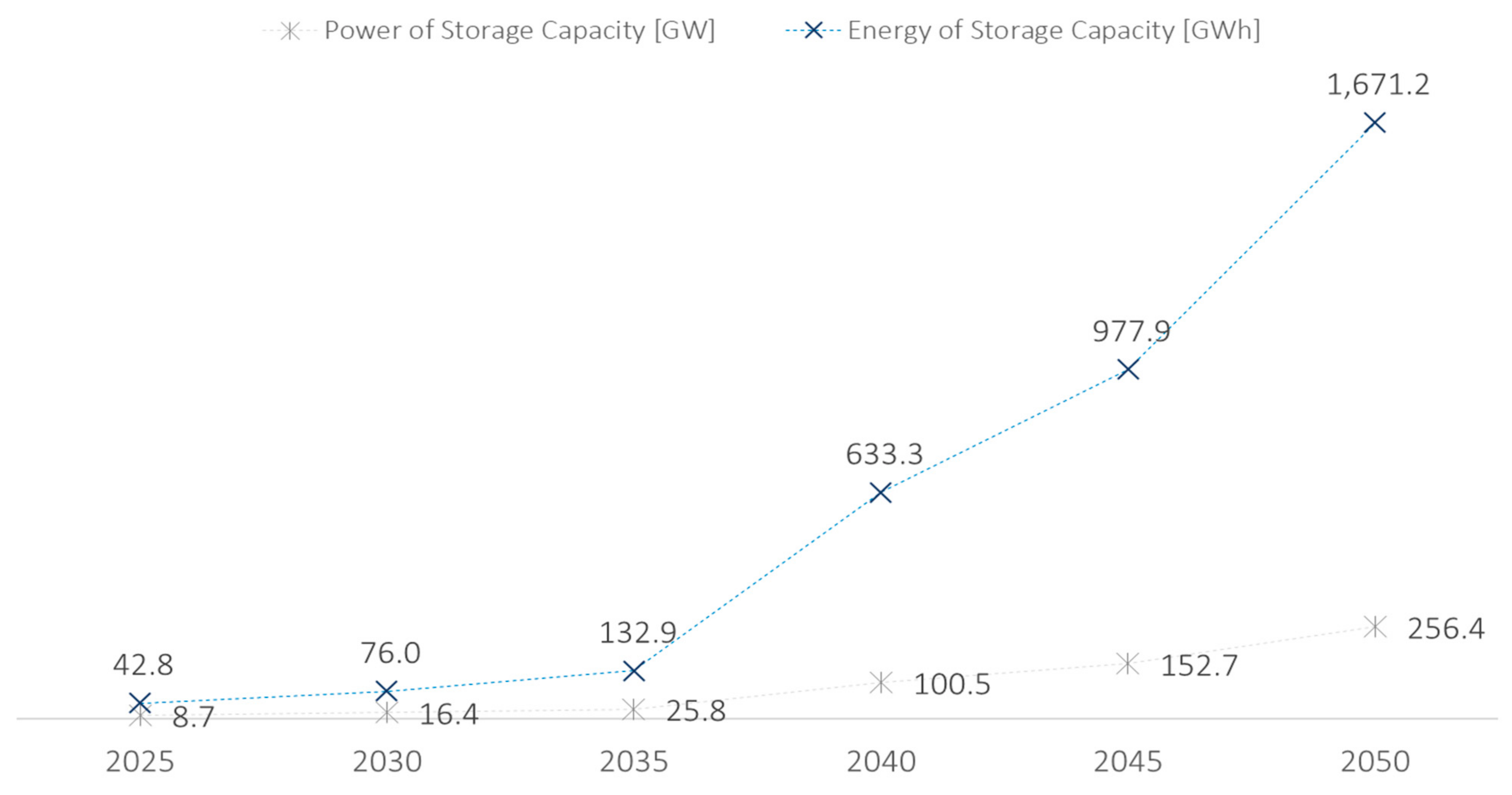
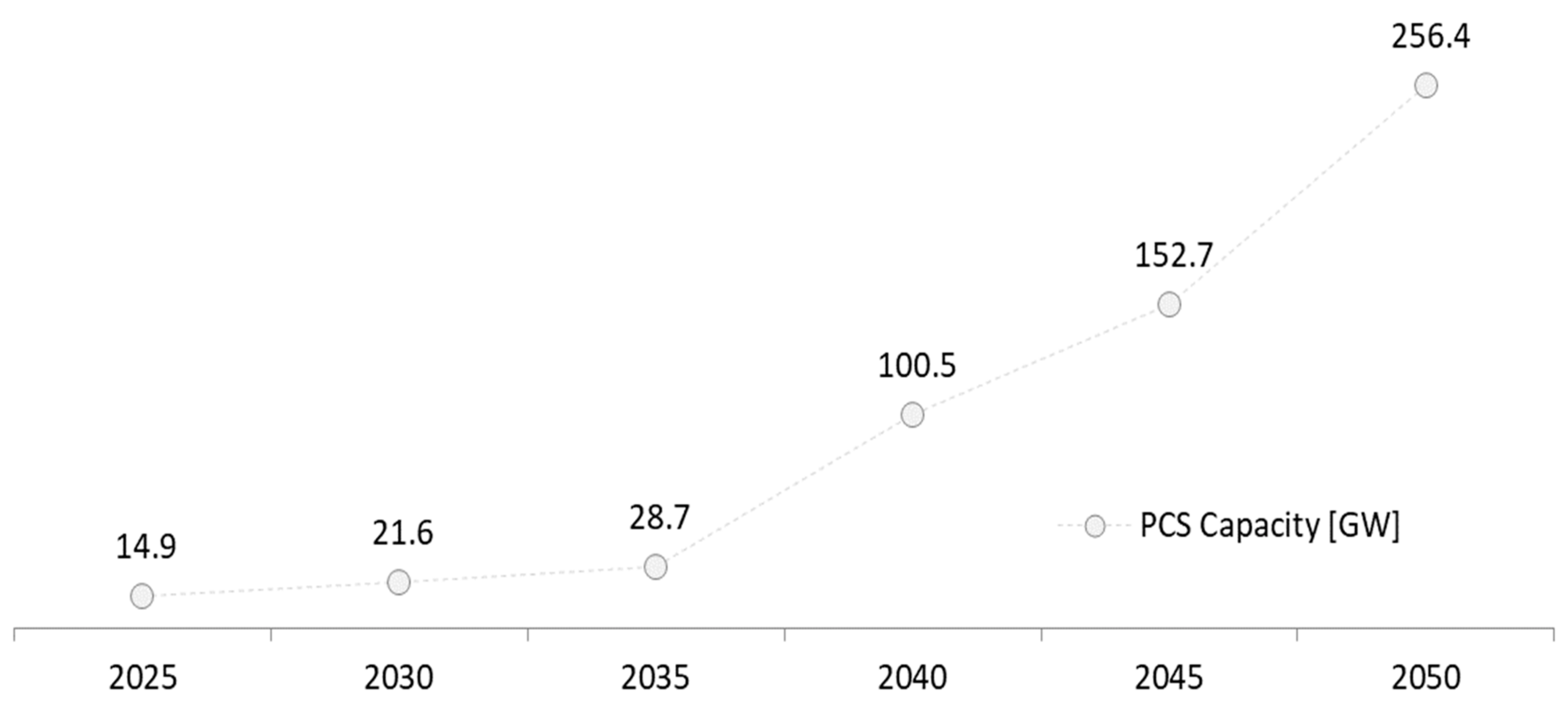
| Total (GW) | 14.9 | 21.6 | 28.7 | 100.5 | 152.7 | 256.4 |
| 2025 | 2030 | 2035 | 2040 | 2045 | 2050 | |
|---|---|---|---|---|---|---|
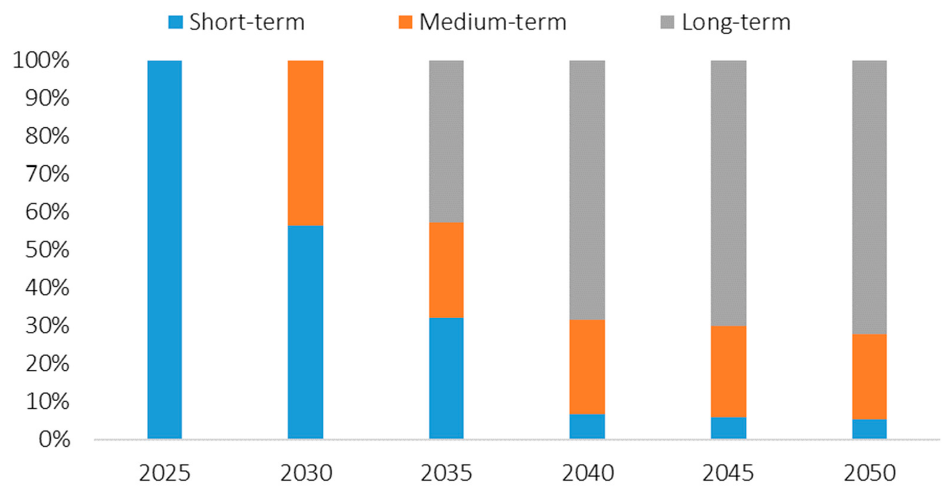
| Short term (GWh) | 42.8 (100%) | 42.8 (56.3%) | 42.8 (32.2%) | 42.8 (6.8%) | 59.0 (6.0%) | 88.7 (5.3%) |
| Medium term (GWh) | - | 33.2 (43.7%) | 33.2 (25.0%) | 156.7 (24.7%) | 233.5 (23.9%) | 378.0 (22.6%) |
| Long term (GWh) | - | - | 56.9 (42.8%) | 433.8 (68.5%) | 685.5 (70.1%) | 1204.5 (72.1%) |
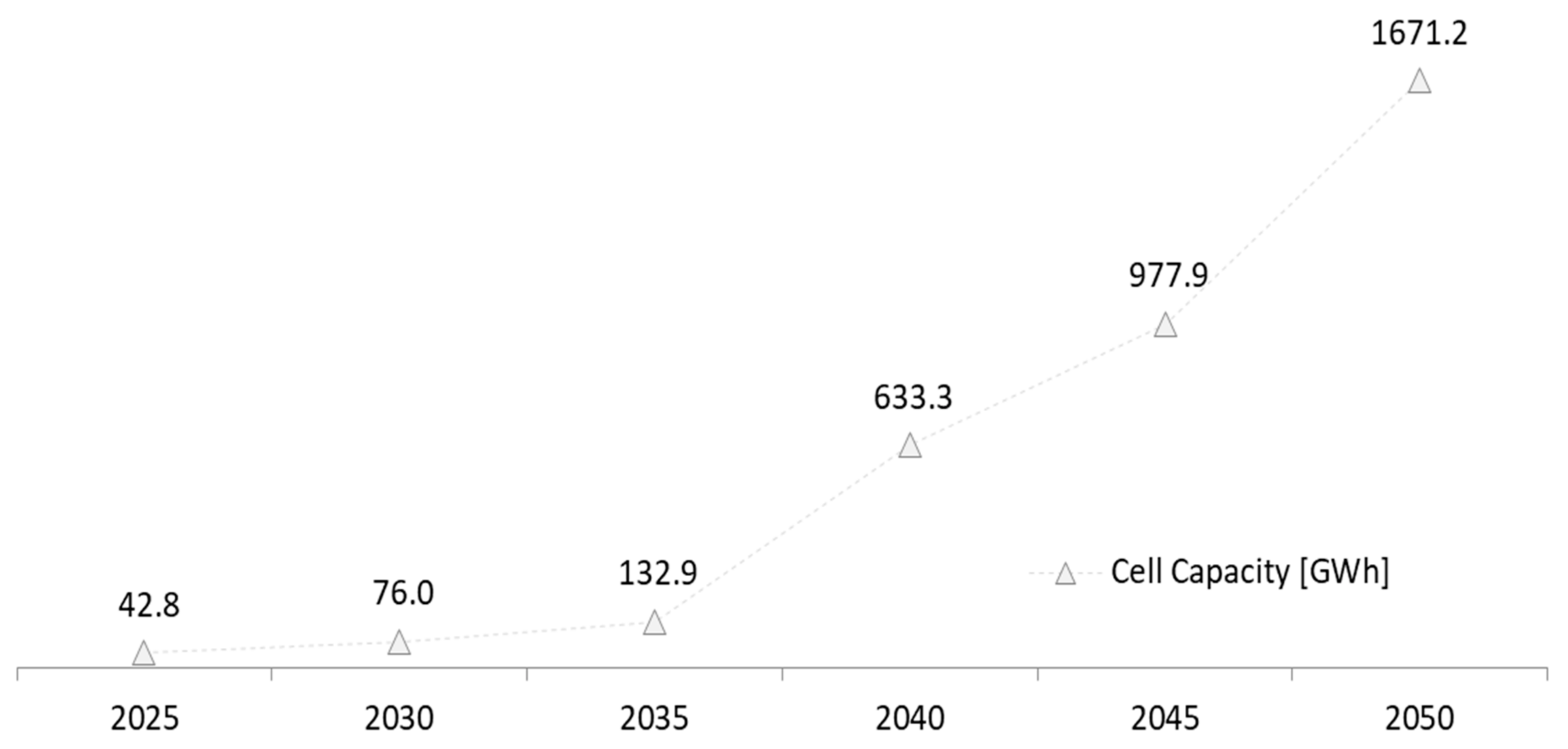
| Total (GWh) | 42.8 | 76.0 | 132.9 | 633.3 | 977.9 | 1671.2 |
| Time Sequence Analysis Result | Snapshot Analysis Result | |
|---|---|---|
| Short term (GW) | 30.2 | 76.0 |
| Medium term (GW) | 75.6 | 0.0 |
| Long term (GW) | 150.6 | 180.4 |
| Total (GW) | 256.4 | 256.4 |
| Time Sequence Analysis Result | Snapshot Analysis Result | |
|---|---|---|
| Short term (GWh) | 88.7 | 228.0 |
| Medium term (GWh) | 378.0 | 0 |
| Long term (GWh) | 1204.5 | 1443.2 |
| Total (GWh) | 1671.2 | 1671.2 |
Disclaimer/Publisher’s Note: The statements, opinions and data contained in all publications are solely those of the individual author(s) and contributor(s) and not of MDPI and/or the editor(s). MDPI and/or the editor(s) disclaim responsibility for any injury to people or property resulting from any ideas, methods, instructions or products referred to in the content. |
© 2023 by the authors. Licensee MDPI, Basel, Switzerland. This article is an open access article distributed under the terms and conditions of the Creative Commons Attribution (CC BY) license (https://creativecommons.org/licenses/by/4.0/).
Share and Cite
Lee, J.; Jung, S.; Lee, Y.; Jang, G. Energy Storage Mix Optimization Based on Time Sequence Analysis Methodology for Surplus Renewable Energy Utilization. Energies 2023, 16, 6031. https://doi.org/10.3390/en16166031
Lee J, Jung S, Lee Y, Jang G. Energy Storage Mix Optimization Based on Time Sequence Analysis Methodology for Surplus Renewable Energy Utilization. Energies. 2023; 16(16):6031. https://doi.org/10.3390/en16166031
Chicago/Turabian StyleLee, Jaegul, Solyoung Jung, Yongseung Lee, and Gilsoo Jang. 2023. "Energy Storage Mix Optimization Based on Time Sequence Analysis Methodology for Surplus Renewable Energy Utilization" Energies 16, no. 16: 6031. https://doi.org/10.3390/en16166031
APA StyleLee, J., Jung, S., Lee, Y., & Jang, G. (2023). Energy Storage Mix Optimization Based on Time Sequence Analysis Methodology for Surplus Renewable Energy Utilization. Energies, 16(16), 6031. https://doi.org/10.3390/en16166031