Graph Complexity Reduction of Exergy-Based FDI—A Tennessee Eastman Process Case Study

Abstract

When applying graph-based fault detection and isolation (FDI) methods to the attributed graph data of large and complex industrial processes, the computational abilities and speed of these methods are adversely affected by the increased complexity. This paper proposes and evaluates five reduction techniques for the exergy-graph-based FDI method. Unlike the graph reduction techniques available in literature, the reduction techniques proposed in this paper can easily be applied to the type of attributed graph used by graph-based FDI methods. The attributed graph data of the Tennessee Eastman process are used in this paper since it is a popular process to use for the evaluation of fault diagnostic methods and is both large and complex. To evaluate the proposed reduction techniques, three FDI methods are applied to the original attributed graph data of the process and the performance of these FDI methods used as control data. Each proposed reduction technique is applied to the attributed graph data of the process, after which all three FDI methods are applied to the reduced graph data to evaluate their performance. The FDI performance obtained with reduced graph data is compared to the FDI performance using the control data. This paper shows that, using the proposed graph reduction techniques, it is possible to significantly reduce the size and complexity of the attributed graph of a system while maintaining a level of FDI performance similar to that achieved prior to any graph reduction.

1. Introduction

Industrial processes play a vital role in the modern world and, as such, must produce a product that meets the necessary quality standards while operating according to the relevant safety guidelines [1]. For this to be accomplished, the control systems must be quite robust and identify faulty operational conditions as quickly as possible. By doing this, it becomes possible to remove the effects of the fault condition or to alert an operator to the faulty operation. A fault detection and isolation (FDI) scheme can be used to detect and identify fault conditions in an industrial system. This scheme is capable of detecting the presence of a fault and then determining which fault has occurred. This allows the system to be diagnosed quickly and accurately and the appropriate corrective action to be taken.

Over the years, a wide variety of FDI methods have been developed based on models and data to effectively detect and isolate faults [2,3,4]. Despite this, none of the individual methods are capable of meeting all the criteria of a fault-diagnostic system. This has led to the emergence of hybrid FDI techniques that blend model-based and data-driven approaches to surpass some of the restrictions of individual methods [3].

One such hybrid method which has shown significant potential is an exergy-based approach outlined by Marais et al. [5]. This method abstracts physical measurements such as pressure and temperature to exergy variables, which are then used for FDI. In the seminal work by Newman and Clauset [6], the notion of capitalising on the network structure of a system to characterise system behaviour is investigated. This work illustrates that network analysis, which borrows ideas from a number of areas, especially graph theory, aims to form a network’s structural features and gain insight on system behaviour. Van Schoor et al. [7] expands on the exergy hybrid approach by using the exergy and energy rate characteristics to create a graph representation of a process. The graph representation is then used for FDI and the technique has been coined the energy-graph-based visualisation (EGBV) approach. The work by Greyling et al. [8] illustrates the usefulness of the technique when applied to a gas-to-liquids process, accounting for both physical and chemical exergy attributes. The work by Wolmarans et al. [9] introduces generalised FDI steps for the EGBV technique and draws a parallel with principal component analysis.

When these graph-based FDI methods are applied to larger and more complex processes, the resulting graph representation of the process is then also significantly more complex. The increased degree of graph complexity makes the implementation of the FDI method more complicated since more process sensor data are required and the mathematical operation performed by the FDI method takes longer to execute [10]. Complex graph representations, therefore, adversely affect the speed of the FDI method, require more resources, and increase the risk of the FDI method being inaccurate.

While there are techniques available in literature that can reduce or summarise attributed graphs to reduce their complexity [11,12,13], these techniques cannot be applied to the type of attributed graphs used by the graph-based FDI methods, verbatim. It is, therefore, warranted to develop reduction techniques that can effectively reduce the size and complexity of the attributed graphs relevant to FDI.

The Tennessee Eastman process (TEP) is a well-known industrial benchmark process that was originally developed by the Eastman Chemical Company. This process model was initially implemented in FORTRAN code to generate simulated process data for advanced process control studies. The process model has become increasingly useful for verifying the performance of various Fault Detection and Diagnosis (FDD) studies [14]. As time passed, this process model was updated and converted to a MATLAB Simulink^® model [15]. Numerous research studies on FDD use this model to benchmark FDD techniques [16]. Furthermore, several studies incorporate graph-theoretic methods as a means of improving the diagnostic performance of the techniques [17].

This paper proposes and evaluates graph reduction techniques that can be used to reduce the size and complexity of the graph representation of a process while maintaining a similar level of FDI performance achieved with the original graph. For each reduction technique, three FDI methods are applied to the subsequently reduced graph data to evaluate the effectiveness of the reduction techniques. The results of this evaluation allow for the comparison of the proposed reduction techniques. An in-house MATLAB Simulink^® model of the TEP is used as a case study for the evaluation of the graph reduction techniques as it represents a large, complex system [18].

Section 2 contains a brief overview of the TEP, after which the three FDI methods used for the evaluation are introduced and discussed in Section 3. Section 4 outlines the graph reduction techniques as proposed in this paper. The results from the evaluation of the reduction techniques are provided in Section 5, which is followed by a section on combining individual reduction techniques in Section 6. Section 7 presents the concluding remarks.

2. Tennessee Eastman Bench Mark Process

The Tennessee Eastman process (TEP) is a model of an industrial chemical plant that is often used as a benchmark to evaluate fault diagnosis techniques. This process model was first proposed in the paper by Downs and Vogel [14]. In this study, the TEP model is used to generate healthy and faulty system data sets and to evaluate graph reduction techniques. The TEP is characterised by two simultaneous gas–liquid reactions and two additional byproduct reactions. These reactions are all exothermic and irreversible. The two gas–liquid reactions are given by:

$$A\left(g\right)+C\left(g\right)+D\left(g\right)\to G\left(liq\right),$$

(1)

$$A\left(g\right)+C\left(g\right)+E\left(g\right)\to H\left(liq\right).$$

(2)

The TEP diagram can be seen in Figure 1 [18]. The process constitutes five main units, which are the reactor, condenser, vapour–liquid separator, compressor, and stripper. Twelve valves can be manipulated in the process, and forty-one process measurements can be taken to control or monitor process operations. The process has 20 possible fault conditions and 21 process conditions when the normal operating condition (NOC) is considered.

Table 1. Fault conditions of the TEP [19].

Fault ID	Fault Description	Type of Change Introduced
Fault 1	A/C feed ratio, B composition constant (stream 4)	Step
Fault 2	B composition, A/C feed ration constant (stream 4)	Step
Fault 3	D feed temperature (stream 2)	Step
Fault 4	Reactor cooling water inlet temperature	Step
Fault 5	Condenser cooling water inlet temperature	Step
Fault 6	A feed loss (stream 1)	Step
Fault 7	C header pressure loss-reduced availability (stream 4)	Step
Fault 8	A, B, C feed composition (stream 4)	Random variation
Fault 9	D feed temperature (stream 2)	Random variation
Fault 10	C feed temperature (stream 4)	Random variation
Fault 11	Reactor cooling water inlet temperature	Random variation
Fault 12	Condenser cooling water inlet temperature	Random variation
Fault 13	Reaction kinetics	Slow drift
Fault 14	Reactor cooling water valve	Sticking
Fault 15	Condenser cooling water valve	Sticking
Fault 16	Unknown	Unknown
Fault 17	Unknown	Unknown
Fault 18	Unknown	Unknown
Fault 19	Unknown	Unknown
Fault 20	Unknown	Unknown

presents an overview of the 20 fault conditions of the TEP. Fault conditions 1 to 7 are as a result of a step change in the process variable associated with each fault. Fault conditions 8 to 12 are as a the result of random fluctuations in the process variable associated with each fault. Fault condition 13 replicates a gradual drift in the kinetics of the process reactions. Fault conditions 14 and 15 are due to stuck valves, and fault conditions 16 to 20 are caused by unidentified faults.

The original process was developed in FORTRAN and was adapted for Simulink^® by Vosloo et al. in [18]. The data generated by this Simulink^® model is used for this study.

For each process condition, the Simulink^® model generates time series data that represent a 25 h period. Process measurements are taken every 180 s, resulting in 501 measurements per condition. For every 25 h period, the first hour represents the NOC after which the process condition is introduced.

3. Graph-Based FDI

In the context of this paper, a graph can be defined as a set of nodes and a set of links, where each link connects two nodes [20]. Graph-based FDI methods require a graph representation of the process in the form of an attributed graph. An attributed graph is a graph that has information assigned to its nodes and/or links [21].

The energy-attributed graph is composed by regarding each main system component as a node with the links describing the energy interactions between the components. The node attributes are chosen to be the rate of exergy change across a node, denoted as $\Delta {\dot{B}}_i$ with i signifying the specific node. The link attributes are chosen to be the energy flow rate between nodes denoted by ${\dot{E}}_{i,j}$ with $i,j$ signifying the location between nodes i and j and the direction from i to j.

Assuming a total of n nodes, a node signature matrix ${\mathbf{N}}_s\in {\mathbb{R}}^{n\times n+1}$, with subscript s denoting the term signature, is given by:

$$\begin{array}{cccc}& \stackrel{\mathrm{Node} \mathrm{attr}.}{︷}& & \stackrel{\mathrm{Link}\mathrm{attr}.}{︷}\\ {\mathbf{N}}_s=& [\begin{array}{c}\Delta {\dot{B}}_1\\ \Delta {\dot{B}}_2\\ ⋮\\ \Delta {\dot{B}}_i\\ ⋮\\ \Delta {\dot{B}}_n\end{array} & |& \begin{array}{cccccc}{\dot{E}}_{1,1}& {\dot{E}}_{1,2}& \cdots & {\dot{E}}_{1,j}& \cdots & {\dot{E}}_{1,j}\\ {\dot{E}}_{2,1}& & & & & \\ ⋮& & \ddots & & & \\ {\dot{E}}_{i,1}& & & {\dot{E}}_{i,j}& & \\ ⋮& & & & \ddots & \\ {\dot{E}}_{n,1}& & & & & {\dot{E}}_{n,n}\end{array}]\end{array}$$

(3)

For nodes between which no energy interaction is taking place, the link attribute is made zero.

Online process monitoring requires the calculation of (3) for every k time instant, i.e., calculating ${\mathbf{N}}_{s,k}$. Furthermore, the calculation of ${\mathbf{N}}_{s,ref}$ is required, a reference node signature matrix composed with energy and exergy attributes of either the desired normal operating condition (NOC) of the process or known fault conditions. Continuously comparing ${\mathbf{N}}_{s,k}$ with the NOC reference matrix ${\mathbf{N}}_{s,refN}$ would reveal undesired process deviations, or faults, thus enabling fault detection. Continuously comparing ${\mathbf{N}}_{s,k}$ and a set of reference matrices which include both ${\mathbf{N}}_{s,refN}$ and known fault conditions ${\mathbf{N}}_{s,refFq}$ would enable characterising the differences in order to conduct fault isolation.

The attributed graph of the TEP can be seen in Figure 2. A summary of the TEP attributed graph nodes and their corresponding process components is given in

Table 2. TEP attributed graph nodes and their corresponding process components.

Process Component	Node Number	Process Component	Node Number
Feed stream A	Node 1	Feed stream D	Node 2
Feed stream E	Node 3	Feed stream A/B/C	Node 4
Mixing zone	Node 5	Reactor	Node 6
Reactor cooling bundle	Node 7	Condenser	Node 8
Condenser cooling side	Node 9	Vapour-liquid separator	Node 10
Purge stream	Node 11	Compressor	Node 12
Stripper	Node 13	Product stream	Node 14
Environment	Node 15	-

. As the process data from the TEP model is available in windows of 501 samples, 501 operational attributed graphs are available for each of the 21 process conditions mentioned in Section 2, i.e., 20 fault conditions and the NOC.

The three FDI methods used in this study are the distance parameter, eigendecomposition, and residual-based FDI methods. Each of these methods requires a reference attributed graph for each of the 21 process conditions. The reference attributed graph (${\mathbf{N}}_{s,ref}$) of a process condition is calculated by determining the average of all 501 operational attributed graphs for that condition.

For both the distance parameter and eigendecomposition FDI methods, the graph comparison process takes the form of the first step of graph matching according to the method described by Jouli et al. [22], using the heterogeneous euclidean overlap metric (HEOM). The comparison of ${\mathbf{N}}_{s,ref}$ and ${\mathbf{N}}_{s,k}$ therefore results in a cost matrix ${\mathbf{C}}_k\in {\mathbb{R}}^{n\times n}$ with its entries $c_{ij,k}$ given by:

$$c_{ij,k}=\sqrt{\sum _{a=1}^{n+1}{\left[\frac{|{\mathbf{N}}_{s,ref}(i,a)-{\mathbf{N}}_{s,k}(j,a)|}{{\left\{range\right\}}_a}\right]}^2},$$

(4)

with a the corresponding attribute number of nodes i and j being compared and

$${\left\{range\right\}}_a=|ma{x}_a-mi{n}_a|,$$

(5)

the range of the corresponding attribute in the reference graph. If the result of (5) is zero, then ${\left\{range\right\}}_a$ is set to be equal to one. The matrix ${\mathbf{C}}_k$ acts as a distance descriptor between ${\mathbf{N}}_{s,ref}$ and ${\mathbf{N}}_{s,k}$. Using (4) to compare ${\mathbf{N}}_{s,ref}$ with itself will result in ${\mathbf{C}}_{ref}$, which acts as the reference distance descriptor for the particular reference whether NOC or a known fault condition.

The distance parameter FDI method makes use of cost matrices that result from a comparison of an operational graph ${\mathbf{N}}_{s,k}$ with all 21 ${\mathbf{N}}_{s,ref}$ for FDI as portrayed in Figure 3. Each cost matrix in the resulting set of matrices (seen in the bottom grid of Figure 3) can then be quantified as a single parameter known as the distance parameters ($DC$). For the square cost matrix resulting from the EGBV method, the distance parameter is merely the average of the diagonal entries of the resulting cost matrix. By observing how the distance parameter of each operational cost matrix relates to the distance parameters of every reference cost matrix, the operational condition can be matched to the appropriate fault condition.

Figure 4 [19] shows how the eigendecomposition FDI method compares reference and operational conditions for FDI. The method compares the reference normal attributed graph (${\mathbf{N}}_{s,refN}$) with itself and the reference faulty attributed graphs (${\mathbf{N}}_{s,refFq}$) to generate a set of 21 cost matrices (Array A in Figure 4) based on this comparison. Eigendecomposition of these cost matrices results in 21 sets of reference eigenvalues (${\overrightarrow{\lambda }}_{Ref}$). Next, the method compares the reference normal attributed graph (${\mathbf{N}}_{s,refN}$) with an operational attributed graph (${\mathbf{N}}_{s,k}$) and generates a single cost matrix (Array B in Figure 4) based on this comparison. Upon eigendecomposition of the resulting cost matrix, a set of operational eigenvalues (${\overrightarrow{\lambda }}_k$) is generated. This operational set of eigenvalues is matched with one of the 21 reference sets of eigenvalues most similar to itself.

The illustration of Figure 4 [19] also applies to the residual-based FDI method. The method firstly compares the reference normal attributed graph (${\mathbf{N}}_{s,refN}$) with itself and the reference faulty attributed graphs (${\mathbf{N}}_{s,refFq}$). It then quantifies the resulting residual matrices as 21 reference binary matrices ($BI{N}_{ref}$) (contained in Array A in the figure) with statistical operations and creates a set of 21 reference frequency vectors (${\overrightarrow{fc}}_{NRef}$), each of which indicates the number of "1’s” in each column of its corresponding binary matrix ($BI{N}_{ref}$). The method then proceeds to compare the reference normal attributed graph (${\mathbf{N}}_{s,refN}$) with an operational attributed graph (${\mathbf{N}}_{s,k}$). It quantifies the resulting residual matrix as an operational binary matrix ($BI{N}_{OP}$) (contained in Array B seen in the figure) with statistical operations and creates an operational frequency vector (${\overrightarrow{fc}}_{NO}$), which indicates the number of “1’s” in each column of ($BI{N}_{OP}$). Finally, the method matches this operational frequency vector with one of the twenty-one reference frequency vectors most similar to the operational binary matrix to diagnose the faulty condition. In essence, these FDI methods mathematically determine the difference between an operational attributed graph and a group of reference attributed graphs. The distance parameter and eigendecomposition FDI methods express these mathematical differences in the form of a cost matrix. The distance parameter FDI method quantifies the cost matrix as a single distance parameter to determine which reference graph best represents the operational graph, while the eigendecomposition method quantifies the cost matrix as a set of eigenvalues to accomplish this goal. For the residual-based FDI method, the mathematical differences are encapsulated in a residual matrix and are ultimately quantified as frequency vectors to match the operational graph with its corresponding reference graph. The overall detection rate represents the average percentage of instances where a fault condition was present in the system and the FDI method detected that a fault was present. The overall isolation rate represents the average percentage of instances a fault condition was present and the FDI method correctly isolated that condition to its corresponding reference condition. The performance of the three FDI methods applied to the TEP attributed graph data can be seen in

Table 3. Summary of the detection and isolation performance of the three FDI schemes applied to the TEP [19].

Distance Parameter FDI Method		Eigendecomposition FDI Method		Residual-Based FDI Method
Overall detection rate (%)	89.81	Overall detection rate (%)	96.28	Overall detection rate (%)	98.86
Overall isolation rate (%)	19.90	Overall isolation rate (%)	17.55	Overall isolation rate (%)	20.15
Isolation of Fault 1 (%)	75.00	Isolation of Fault 1 (%)	90.00	Isolation of Fault 1 (%)	80.00
Isolation of Fault 2 (%)	85.00	Isolation of Fault 2 (%)	75.00	Isolation of Fault 2 (%)	61.00
Isolation of Fault 6 (%)	59.00	Isolation of Fault 6 (%)	100.00	Isolation of Fault 6 (%)	88.00

. These performance indicators will be used as a set of control data when evaluating the graph reduction techniques. Certain well-performing specific isolation rates are highlighted for each FDI method.

4. Graph Reduction Techniques Description

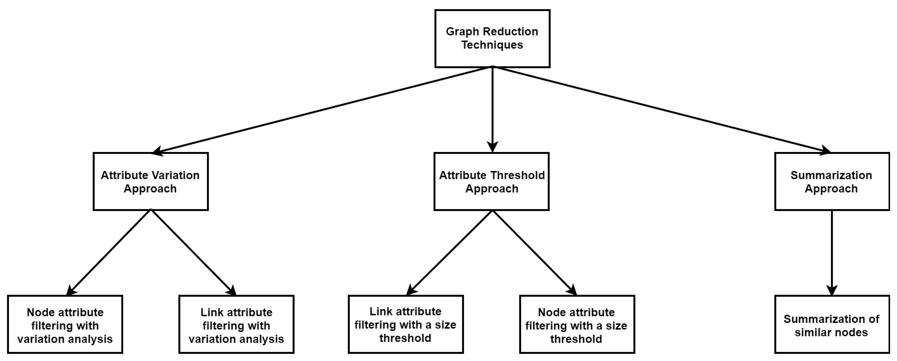
This study proposes five reduction techniques that were formulated from three principal approaches based on techniques found in the literature, as well as an understanding of how FDI methods detect and isolate fault conditions. The tree diagram depicted in Figure 5 illustrates how the three principal approaches branch off into five different techniques. The first principal approach (Attribute Variation Approach) determines the degree to which graph attributes under NOC vary when fault conditions are introduced into the process. The rationale for this strategy is that attributes that experience little change during a fault situation have a minimal impact on the cost or residual matrices used by FDI techniques and can be removed from the attributed graph information. Algorithm 1 represents the technique that results from applying the first principal approach to node attributes, while Algorithm 2 represents the resulting technique from applying the first principal approach to link attributes.

The second technique involves recognising attributes with relatively small values under NOC and eliminating them from the attributed graph data. This approach is based on the idea that attributes that are quite smaller compared to all the other graph attributes under NOC have a much smaller impact on the cost or residual matrices utilised by the FDI methods. The first and second approaches discussed up to now take into account node and link attributes individually, thus having two distinct techniques for each. Algorithm 3 is the resulting technique from applying the second principal approach to link attributes, while Algorithm 4 represents the resulting technique from applying the second principal approach to node attributes.

The final principal approach identifies nodes that have similar attribute values and summarises those nodes into a single node. The logic underpinning this approach is that, by summarising similar nodes, the structural size of the attributed graph is reduced, while all the attributes are retained. This, in theory, has a negligibly small effect on the FDI method and will not disrupt FDI performance too severely.

Table 4. Summary of the graph reduction techniques [19].

Technique Number	Name	Reduction Type	Description
1	Node attribute filtering with variation analysis	Node attribute	Eliminates node attributes based on their average variation from NOC over all fault conditions.
2	Link attribute filtering with variation analysis	Link attribute	Eliminates link attributes based on their average variation from NOC over all fault conditions.
3	Link attribute filtering with a size threshold	Link attribute	Eliminates link attributes based on the magnitude of the attributes in NOC.
4	Node attribute filtering with a size threshold	Node attribute	Eliminates node attributes based on the magnitude of the attributes in NOC.
5	Summarisation of similar nodes	Node attribute	Combines nodes that are alike into one node by summarising their attributes.

contains a summary of all five techniques with a brief discussion of each technique. Algorithm 5 is the technique that results from applying the final principal approach to summarise node attributes.

Algorithm 1 Node attribute filtering with variation analysis

Calculate how much each node varies from NOC for the 20 fault conditions. The physical and chemical exergy values of a node are summated. for$i\in [1,2,\dots ,14]\mathbf{do}$  for$j\in [1,2,\dots ,20]\mathbf{do}$   $Temp+=$$|N_{s,refN}(i,1:2)-N_{s,refF}\left(j\right)(i,1)|$  end for  $Avg\_Variation\left(i\right)=(Temp/N_{s,refN}(i,1))\times 100$ end for Arrange nodes into percentiles according to their percentage variation from NOC values. Use MATLAB’s ‘isoutlier()’ function to remove a percentile of nodes, iteratively. Start with the percentile of nodes with the smallest variation. $N_{Reduced}=N_{Original}$ for$k\in [1,2,\dots ,10]\mathbf{do}$  $N_{Reduced}\leftarrow isoutlier\left(N_{Reduced}\right)$  $FDI\left(N_{Reduced}\right)$ end for

Algorithm 2 Link attribute filtering with variation analysis

Calculate how much each link varies from NOC for the 20 fault conditions. for$i\in [1,2,\dots ,15]\mathbf{do}$  for$j\in [1,2,\dots ,15]\mathbf{do}$   for$k\in [1,2,\dots ,20]\mathbf{do}$    $Temp+=$$|N_{s,refN}(i,j+2)-N_{s,refF}\left(k\right)(i,j+2)|$   end for  $Avg\_Variation(i,j)=(Temp/N_{s,refN}(i,j+2))\times 100$  end for end for Arrange links into percentiles according to their percentage variation from NOC values. Use MATLAB’s ‘isoutlier()’ function to remove a percentile of links, iteratively. Start with the percentile of links with the smallest variation. $N_{Reduced}=N_{Original}$ for$m\in [1,2,\dots ,10]\mathbf{do}$  $N_{Reduced}\leftarrow isoutlier\left(N_{Reduced}\right)$  $FDI\left(N_{Reduced}\right)$ end for

Algorithm 3 Link attribute filtering with a size threshold

Arrange links into percentiles according to the size of their attribute values. Use MATLAB’s ‘isoutlier()’ function to remove a percentile of links, iteratively. Start with the percentile of nodes with the smallest values. $N_{Temp}=N_{s,refN\_avg}(1:15,3:17)$ for$m\in [1,2,\dots ,10]\mathbf{do}$  $N_{Reduced}\leftarrow isoutlier\left(N_{Temp}\right)$  $N_{Temp}=N_{Reduced}$  $FDI\left(N_{Reduced}\right)$ end for

Algorithm 4 Node attribute filtering with a size threshold

Arrange nodes into percentiles according to the size of their attribute values. Use MATLAB’s ‘isoutlier()’ function to remove a percentile of nodes, iteratively. The physical and chemical exergy values of a node are summated. Start with the percentile of nodes with the smallest values. $N_{Temp}=N_{s,refN}(1:14,1:2)$ for$m\in [1,2,\dots ,10]\mathbf{do}$  $N_{Reduced}\leftarrow isoutlier\left(N_{Temp}\right)$  $N_{Temp}=N_{Reduced}$  $FDI\left(N_{Reduced}\right)$ end for

Algorithm 5 Summarisation of similar nodes

Calculate the difference between each node and all the other system nodes. The physical and chemical exergy values of a node are summed. for$i\in [1,2,\dots ,15]\mathbf{do}$  for$j\in [1,2,\dots ,15]\mathbf{do}$   $Temp(i,j)=$$|N_{s,refN}(i,1:2)-N_{s,refN}(j,1:2)|$  end for end for Identify node pairs which have the smallest attribute differences between them and summarise each pair of nodes into a single node.  $N_{Summarized}\leftarrow min\left(Temp\right)$  $FDI\left(N_{Summarized}\right)$

Link attribute reduction techniques remove a link from the attributed graph by setting the corresponding entry in the node signature matrix (NSM) to zero. Node attribute reduction techniques remove a node from the attributed graph by removing that node’s corresponding row and column from the NSM. All five techniques are restricted from removing the environmental node in order to preserve critical structural information.

5. Results and Discussion

To determine the effectiveness of each graph reduction technique, an experimental evaluation is performed, by which the extent to which each technique reduces the graph data is increased incrementally and the performance of the FDI methods applied on the subsequently reduced data is measured, recorded with each iteration. For Techniques 1–4, the reduction intervals are represented by percentiles, and as the reduction interval increases, the percentile of attributes to be reduced is also increased. For Technique 5, the reduction intervals are represented by the number of summarisations (also referred to as the number of mergers), and as the reduction interval increases, the number of mergers is increased.

Consider, for example, Technique, 1 which is a node attribute reduction technique that reduces attributes according to the average amount they vary from NOC as fault conditions occur. The attributes are sorted into percentiles according to their average variation from NOC. For the first reduction iteration, all the attributes with average variation values that fall within the 10th percentile are removed from the graph data. Upon the second iteration, the interval is increased to the 20th percentile, and all attributes that lie between the 10th and 20th percentile are also removed. This is repeated until the 90th percentile is reached.

When considering Technique 5, the first iteration summarises one pair of similar nodes. Upon the second iteration, a second pair of similar nodes is also summarised. This is repeated until none of the remaining nodes have a high degree of similarity so as to prevent the structural information of the graph from being distorted too severely. All nodes may only be summarised once.

For the sake of brevity, only overall detection and overall isolation rates are considered in this paper. These two indicators are the most important performance indicators and accurately reflect the efficacy of an FDI method.

5.1. Detection Results

The overall detection rate results of all three FDI methods after evaluating reduction Techniques 1–5 on the TEP graph data are portrayed in Figure 6. Upon inspecting the overall detection rate results in Figure 6, it is firstly clear that, for all reduction techniques, the order of performance remains the same, namely, the residual method gives the best performance, the eigendecompoisition method the second best, and the distance method the worst performance. Furthermore, it is also characteristic that, as the number of attributes reduced becomes greater, the detection accuracy increases. This can be expected since, as the graphs are reduced, unnecessary information that do not contribute to detection are removed, resulting in more accurate fault detection. Upon further inspection of the results, it is clear that, for each graph reduction technique, there was at least one reduction interval where the FDI performance of at least one of the FDI methods maintained a similar level of FDI performance as achieved before reducing any attributes. This indicates that graph reduction is a viable solution to addressing the problems caused by large and complex graph structures.

5.2. Isolation Results

The overall isolation rate results after evaluating reduction Techniques 1–5 on the TEP graph data are portrayed in Figure 7. Techniques 1, 3, and 4 show a clear downward trend as more attributes are reduced. However, Techniques 2 and 5 show promising results with fairly consistent performance as attributes are reduced.

5.3. General Observations

Two types of anomalies could be observed when looking at the trends of the overall detection and isolation rates. The first type is the creation of a local maximum when a downward trend changes to an upward trend as the reduction interval is increased and changes back to a downward trend upon the following reduction interval increase. The second type is the creation of a local minimum when an upward trend changes to a downward trend as the reduction interval is increased, then changes back to an upward trend upon the following reduction interval increase. An example of such an anomaly can be seen in Figure 6d for both the eigendecomposition and residual-based FDI methods once 59.68% of the total number of link attributes present in the original graph have been reduced.

The occurrence of these local minima and maxima can be ascribed to the fact that the graph data contain attribute information that are vital to the FDI process, as well as attribute information that are non-vital to the FDI process. When the upward trend part of either the local minima or maxima occurs, it is the result of the reduction operation removing attributes that negatively impact the FDI process. The downward trend section of either the local minima or maxima occurs due to the reduction operation removing attributes that support the FDI process.

By doing an inter-technique comparison, it is possible to determine which reduction techniques work better than others. When doing this comparison, however, it should be noted that the scales of the x-axes in Figure 6 are not necessarily displayed linearly. By comparing all five reduction techniques, it is clear that attribute variation analysis techniques (Techniques 1 and 2) outperformed the attribute size analysis techniques (Techniques 3 and 4) across all three FDI methods when the same range of reduction is used for the comparison.

It is further evident that, when the effect of Technique 5 on the performance of the FDI methods is compared to that of all four other methods over the same range of reduction, Technique 5 has the most stable and consistent effect on both the overall detection and isolation rates of the FDI methods. This shows that Technique 5 is effective at reducing graph complexity without significantly affecting the performance of the FDI methods. This is expected since, by only summarising attributes, Technique 5 preserves the majority of vital attributes while still reducing complexity.

Each FDI method responded well to certain complementary reduction techniques applied at specific percentile thresholds. The distance parameter FDI method responded well to Techniques 1, 2, and 5 at specific threshold values. Techniques 2 and 5, at specific thresholds, had a favourable effect on the performance of the eigendecomposition FDI method. The residual-based FDI method also had a very good response to Techniques 1, 2, and 5 at specific threshold values.

In seeking validation of the trends reported with the TEP as a case study, the techniques were also evaluated on a gas-to-liquids process model. Similar trends were observed; however, future work is warranted to make more general conclusions [19].

6. Combining Individual Reduction Techniques

After applying each of the five individual reduction techniques to the attributed graph data used by the FDI methods, the efficacy of combining reduction techniques is briefly considered. This is accomplished by identifying complementary reduction techniques (techniques that were able to significantly reduce graph data while still maintaining a similar level of FDI performance) for each FDI method and applying these reduction techniques to the graph data simultaneously. For instance, if Techniques 1 and 2 are identified as complementary to a certain FDI method, and if Technique 1 removes nodes 1 and 3 from the graph data, while Technique 2 removes nodes 5 and 8, then the combined reduction technique removes nodes 1, 3, 5, and 8, and all the links connected to these nodes, from the graph data.

While this paper’s investigation into the efficacy of these combined reduction techniques may not have been extensive, the initial results show that combined approaches have value. By combining Techniques 1, 2, and 5 at certain reduction intervals and applying the distance FDI method to the resulting reduced graph data, the overall detection rate increased, the overall isolation rate remained nearly unchanged, and the FDI execution time decreased by nearly 38% relative to the results obtained from applying this FDI method to the original graph data.

By combining Techniques 2 and 5 at certain reduction intervals and applying the eigendecomposition FDI method to the resulting reduced graph data, the overall detection rate increased by nearly 2%, the overall isolation rate fell by only 0.9%, and the FDI execution time decreased by nearly 61%, relative to the results obtained from applying this FDI method to the original graph data. For the residual-based FDI method, it could be observed that, by combining Techniques 1, 2, and 5 at certain reduction intervals, and applying the FDI method to the reduced graph data, the overall detection rate increased by 0.45%, the overall isolation rate also improved with 0.5%, and the FDI execution time decreased by 42%, relative to the results obtained from applying this FDI method to the original graph data. These results clearly show that using the proposed reduction techniques in specific combinations offer several advantages and thus warrant further investigation.

7. Conclusions

The results as outlined in this paper indicate that it is possible to reduce the attributed graph data of a process and maintain a similar level of FDI performance as achieved before any reduction. By comparing the effectiveness of all five graph reduction techniques over the same reduction range, it can be seen that Techniques 1 and 2, which rely on attribute variation, outperformed Techniques 3 and 4, which rely on attribute size, in terms of detection and isolation capabilities. The comparative investigation also revealed that, out of all five techniques, Technique 5 had the most stable effect on the performance of all three FDI methods. This is because Technique 5 summarises attributes while the four other techniques remove attributes from the graph data. The understanding gained from evaluating these proposed reduction techniques can now be used as the basis for implementing optimisation algorithms, such as a genetic algorithm, to further optimise complex attributed graph structures used for FDI. This study’s findings also hold significant value for future studies concerned with effective sensor placement. Once an effectively reduced version of the attributed graph of a process has been produced, sensors should be deployed in such a way that they primarily measure process data from the components and streams which are present in the reduced version of the attributed graph.