Day-Ahead Dynamic Assessment of Consumption Service Reserve Based on Morphological Filter

Abstract

With the development goal of a low-cost and low-carbon reserve market, this paper proposes a dynamic assessment method for day-ahead consumption service reserve demand considering the forecast error of uncertainty power. The iterative self-organizing data analysis techniques algorithm is adopted to cluster the historical actual power into typical scenarios. In addition, the online matching between the typical scenario and the day-ahead forecast power is conducted. In order to realize the hierarchical quantification of reserve demand, the reserve resources in the whole power system are classified according to their response time. Furthermore, the mathematical morphology filter based on the structural elements that are consistent with the response time of the hierarchical reserve resources is initially applied to decompose the historical forecast error of the matched scenarios. The simulation results verify that the proposed dynamic assessment effectively reduces the reserve cost on the basis of being able to cope with multi-time-scale power fluctuations.

1. Introduction

With the Chinese national energy strategic goals of having carbon dioxide emissions peak before 2030 and achieving carbon neutrality before 2060, China has entered a period of rapid development in wind and photovoltaic power [1]. By the end of 2022, the cumulative installed capacity of wind power and photovoltaic in China will have reached 328 GW and 306 GW, respectively, accounting for 13.8% and 12.9% of the total installed capacity of power generation. In addition, the installed capacity proportions of wind and solar energy in many provinces have already exceeded 30%, which are likely to continue increasing in the future. However, the uncertainty of a new power system with a high proportion of renewable energy is significantly enhanced due to the innate nature of randomness, intermittency, and volatility of wind and photovoltaic power. Compared with the traditional power grid dominated by synchronous power generation, dispatch operators are faced with much more severe challenges of real-time power balance due to the complex and changeable characteristics of system operation [2,3,4].

The reserve refers to dispatchable power with different day-ahead response times preserved to ensure the operational safety and reliability of power supply. At present, the seven major regional electricity markets in the United States are organized by the registered training organization (RTO) or independent system operator (ISO). In general, the major regional markets in the United States divide reserves into spinning reserves (synchronous reserves), non-spinning reserves (non-synchronous reserves), and thirty-minute reserves. Contrastingly, European transmission network operators collectively refer to reserve as balance power, corresponding to the primary frequency response, secondary frequency response, and tertiary frequency response processes. Thus, the reserve plays a crucial role in balancing the forecast deviation of load and renewable energy power, as well as dealing with the real-time imbalance of active power caused by various grid faults and other unpredictable events. Therefore, scientific and rational assessment of reserve demand in the day-ahead power generation plan is the premise to ensure the safe, reliable, and economical operation of power systems.

With the surge in the penetration rate of wind and photovoltaic power, power forecast errors and power fluctuations inevitably exist in current power systems. There have been some studies on reserve assessment [5,6,7,8] aiming at the phenomenon of excessive reserve reservation. A dynamic assessment model of reserve demand with invalid reserve capacity expectation is proposed in [9]. The analysis in [10] shows that the probability density function (PDF) of the reserve demand is consistent with the PDF of wind power deviation. The reserve demand is equal to the upper limit of the integral by integrating the PDF of the forecast deviation to meet the confidence level. A dynamic assessment method for the probability of reserve demand based on non-parametric kernel density estimation is constructed in [11] and the effectiveness of the results is evaluated through indicators such as reserve coverage and invalid reserve rate. An optimization model for quantifying reserve demand under typical scenarios is established in [12] based on the proposed wind ramp events prediction. A flexible dynamic reserve assessment method is proposed in [13], in which non-parametric density estimation and machine learning method are adopted to extract the uncertain part of the day-ahead forecast power to estimate the up- and down-reserve demand.

Dividing the typical scenarios of power fluctuation is an effective way to improve the reasonableness of reserve capacity. For scenario classification methods, some commonly used clustering algorithms include K-means algorithm [14], density-based spatial clustering of applications with noise (DBSCAN) algorithm [15], and hierarchical clustering [16], fuzzy c-means clustering [17], etc. The fuzzy c-means clustering method proposed in [17] divides the wind power cluster based on the dynamic characteristics. The Ng-Jordan-Weiss spectral clustering algorithm combined with K-means is proposed in [18] to classify the load power scenarios. Among the above clustering algorithms, the K-means algorithm is the most commonly used because of its simple principle and easy implementation, but the cluster number of the K-means algorithm is difficult to determine in advance when the sample data are huge and multi-dimensional. Therefore, the iterative self-organizing data analysis techniques algorithm (ISODATA) is applied to tackle the issue. The ISODATA clustering algorithm is adopted in [19] to cluster the load power, demonstrating its superior clustering effect compared to the traditional K-means algorithm.

However, with all the relevant research mentioned above, there are still some technical issues which are yet to be resolved, which are summarized as follows. First, most of the relevant studies on reserve demand assessment focus on the spinning reserve that can be called up within 10 min or the operating reserve that can be called up within 30 min, while hardly considering the fluctuation characteristics of wind and photovoltaic power. Second, in view of the randomness and irregularity of wind power generation, the commonly used K-means clustering algorithm makes it difficult to predetermine the number of clusters. Third, the current reserve demand assessment methods have not fully taken the impact of wind and solar energy power forecast errors into consideration which leads to the incomprehensive reflection of the real reserve demand. In addition, there is little research focusing on the hierarchical and dynamic assessment of reserve demand based on the response time of various dispatch resources.

To address the above problems, this paper innovatively proposes a hierarchical dynamic assessment method for the day-ahead consumption service reserve demand that takes both renewable energy and load forecast errors into account. Compared with the existing works, the main work and contributions of this study are summarized as follows:

(1) The concept of consumption service reserve considering the uncertainty of wind and photovoltaic power is proposed, aiming to deal with the forecast deviation.

(2) The scenario clustering is carried out accordance with historical power based on the ISODATA clustering algorithm without the pre-definition of clustering number. Moreover, the online matching between the typical scenario and the day-ahead forecast data is realized.

(3) The morphology filter is adopted to decompose the historical forecast error of the matched scenarios according to the response time of the system hierarchical reserve resources and realize the extraction of multi-time-scale fluctuation characteristics and decomposition of the uncertainty degree.

The rest of this article is organized as follows: the operation rules of morphological filter and its structural elements selection are introduced in Section 2. The concept of consumption service reserve is proposed, and hierarchical classification of reserve resources is introduced in Section 3.1. The ISODATA clustering algorithm is introduced in Section 3.2, and dynamic assessment of day-ahead consumption service reserve demand is introduced in Section 3.3. Section 4 presents the scenario clustering results and the assessment results of reserve demand.

2. Decomposition of Forecast Error Based on Morphological Filter

2.1. Basic Operations of Mathematical Morphology

The operation of mathematical morphology takes erosion and dilation as the basic operations and leads to common morphological operations such as morphological opening and morphological closing, and the cascade combination of both [20]. Let the domains of one-dimensional discrete input signal $f(n)$ and sequence structure elements $g(m)$ be $D_f=\{x_0,x_1,\cdots x_{N-1}\}$ and $D_g=\{y_0,y_1,\cdots y_{M-1}\}$, respectively, with $N>M$, and the erosion $(\oplus )$ and dilation $(\Theta )$ of $f(n)$ defined as Formula (1) and Formula (2), respectively.

$$(f\Theta g)(n)=\min \{f(n+m)-g(m)\}$$

(1)

$$(f\oplus g)(n)=\max \{f(n-m)+g(m)\}$$

(2)

where, $n+m,n-m\in D_f$, $m\in D_g$.

The shape opening operation can smooth and suppress the peak noise of the signal curve and eliminate the scattered points and burrs of the signal. On the other hand, the closing operation can suppress the trough noise of the signal and fill in the small groove structure in the signal. The geometric meaning of the opening operation and the closing operation is that the structural elements are translated from the top and bottom of the time series to approach the forecast error curve, and the undetectable part will be replaced by the structural element’s own morphological characteristics. The morphological opening and morphological closing operations are defined as Formula (3) and Formula (4), respectively.

$$(f\circ g)(n)=[(f\Theta g)\oplus g](n)$$

(3)

$$(f•g)(n)=[(f\oplus g)\Theta g](n)$$

(4)

where, the symbol of $\circ$ and $•$ represent the morphological opening operation and morphological closing operation, respectively.

The morphological opening-closing (OC) and closing-opening (CO) filters are formed by the cascaded combination of morphological opening and closing operations. These filters have the functions of peak clipping and valley filling, and can simultaneously filter out positive and negative pulse noise in the signal. Due to the anti-expansion of the opening operation and the expansion of the closing operation, the output amplitude of the morphological OC filter is relatively small, while the output amplitude of the morphological CO filter is relatively large. Consequently, neither the OC nor CO filter alone can obtain favorable results. However, the filter formed by the cascade combination of morphological opening and closing operations can filter out different noises on the curve. Therefore, in this paper, the average value of OC and CO operations is used to bring the filtering result closer to the original signal.

$$h_{\mathrm{OCCO}}=0.5\times (f\circ g•g+f•g\circ g)$$

(5)

where, $h_{\mathrm{OCCO}}$ is the average value of the cascaded combination of opening operation and closing operation, $f\circ g•g$ is the morphological OC operation, and $f•g\circ g$ is the morphological CO operation.

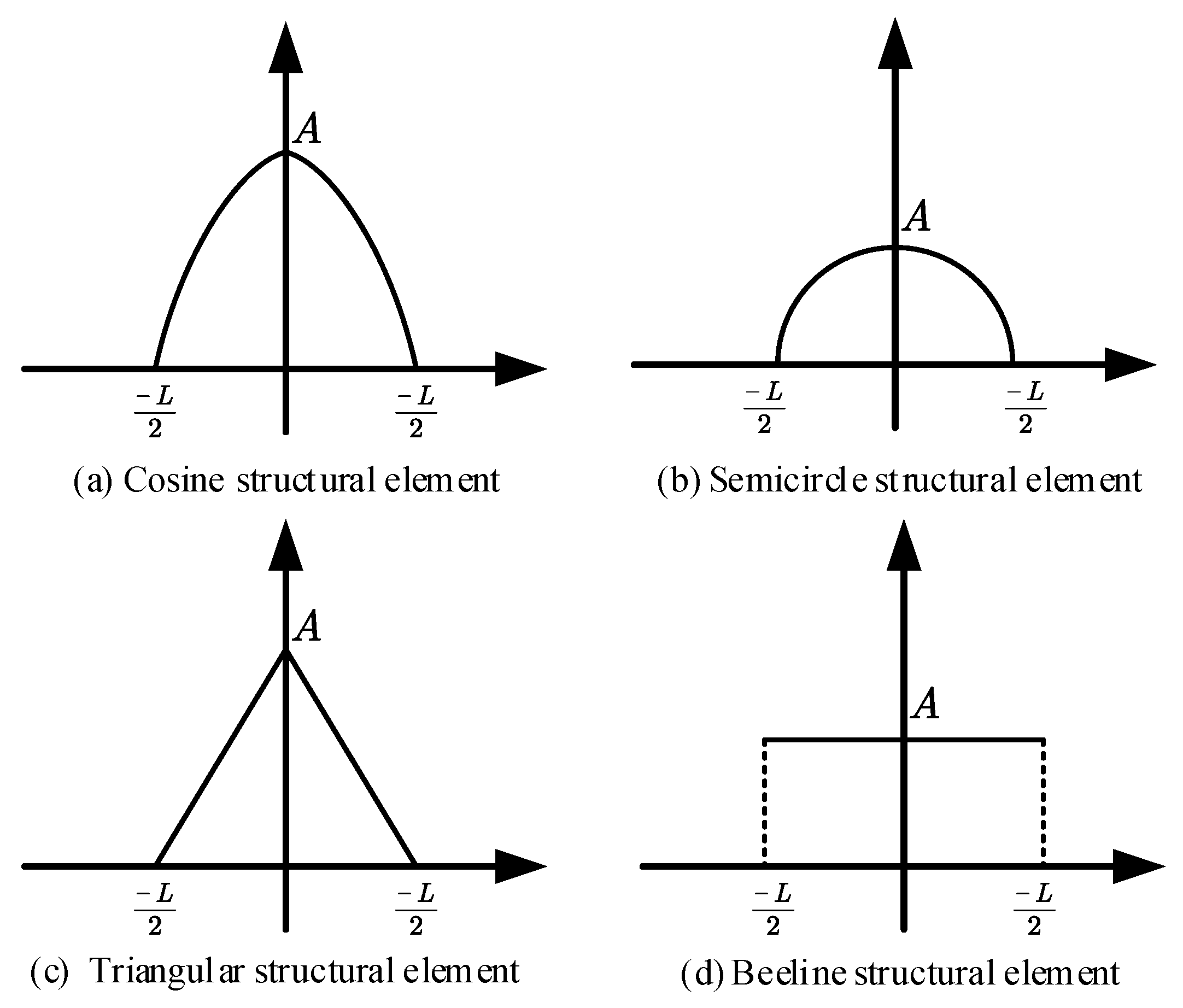
2.2. Selection of Morphological Filter Structural Elements

Once the operation mode of the morphological filter is determined, the shape of the selected structural element becomes the next main factor affecting the output effect of the filter. Commonly used structural elements include cosine, semicircle, triangle, straight line, and their combinations, etc., as shown in Figure 1. The exact shape of each element is determined by the amplitude (A) and width (L). Different selections of the values of A and L can also obtain different filter effects.

The morphology filter is a specific type of cellular automata that modifies the pixel value based on its neighborhood. The neighborhood is referred to as the structured element, which is used to perform set operations such as shift, intersection, and union on the original error curve. By constructing structural elements with different time scale characteristics, it is possible to extract the fluctuation rules of different time periods in the time series. Therefore, the purpose of decomposing historical forecast errors based on the morphological filter is to decompose the forecast error curve into fluctuation components of corresponding time scales by constructing multi-time-scale structural elements.

3. Day-Ahead Dynamic Assessment of Consumption Service Reserve Demand

3.1. Hierarchical Classification of Day-Ahead Reserve Resources

In traditional power grids, the types of reserve include load reserve, frequency containment reserve, and fault reserve. Among them, load reserve is also called peak-shaving reserve, and the demand assessment of load reserve mainly considers the uncertainty caused by load forecast error and load fluctuation. China’s power grid stipulates that the spinning reserve capacity servicing for load forecast error should be 2–5% of the maximum power generation load. According to the regulations of California, the load reserve is 5% of the maximum load during the load steady period; the load reserve is 10% of the maximum load during the load climbing stage. As the penetration rate of wind and solar energy continues to increase, the traditional reserve type is no longer able to cope with the forecast error caused by their strong uncertainty. Therefore, a power grid with a high proportion of wind and solar energy should increase the corresponding consumption reserve to accommodate the expanding deviation between forecast power and the actual output power of wind and solar energy.

Power reserve is categorized into up-reserve and down-reserve: up-reserve, also called spinning reserve, refers to the power that can be put into grid operation immediately, while the power that can be quickly withdrawn is down-reserve. The accurate assessment of reserve requirements is based on reasonable reserve classification criteria. Considering the performance of various units, the regulation resources are classified into automatic generation control (AGC) frequency modulation reserve, 10 min spinning reserve, 30 min reserve, and 60 min reserve according to the response time characteristics [21].

Table 1. Frequency adjustment and alternate resources.

Alternate Resources	Response Time	Unit Type
Primary regulatory resources (AGC)	<5 min	Gas-fired units, fast coal-fired units, pumped storage power, and cascade hydropower station.
Secondary regulatory resources	<10 min	Gas-fired units, fast coal-fired units, pumped storage power station, and cascade hydropower station.
Tertiary regulatory resources	<30 min	Slow coal-fired unit and single cycle gas unit.
Four levels of regulatory resources	>60 min	Combined cycle gas turbine in warm start.

shows the classification results of reserve resources with multiple time scales.

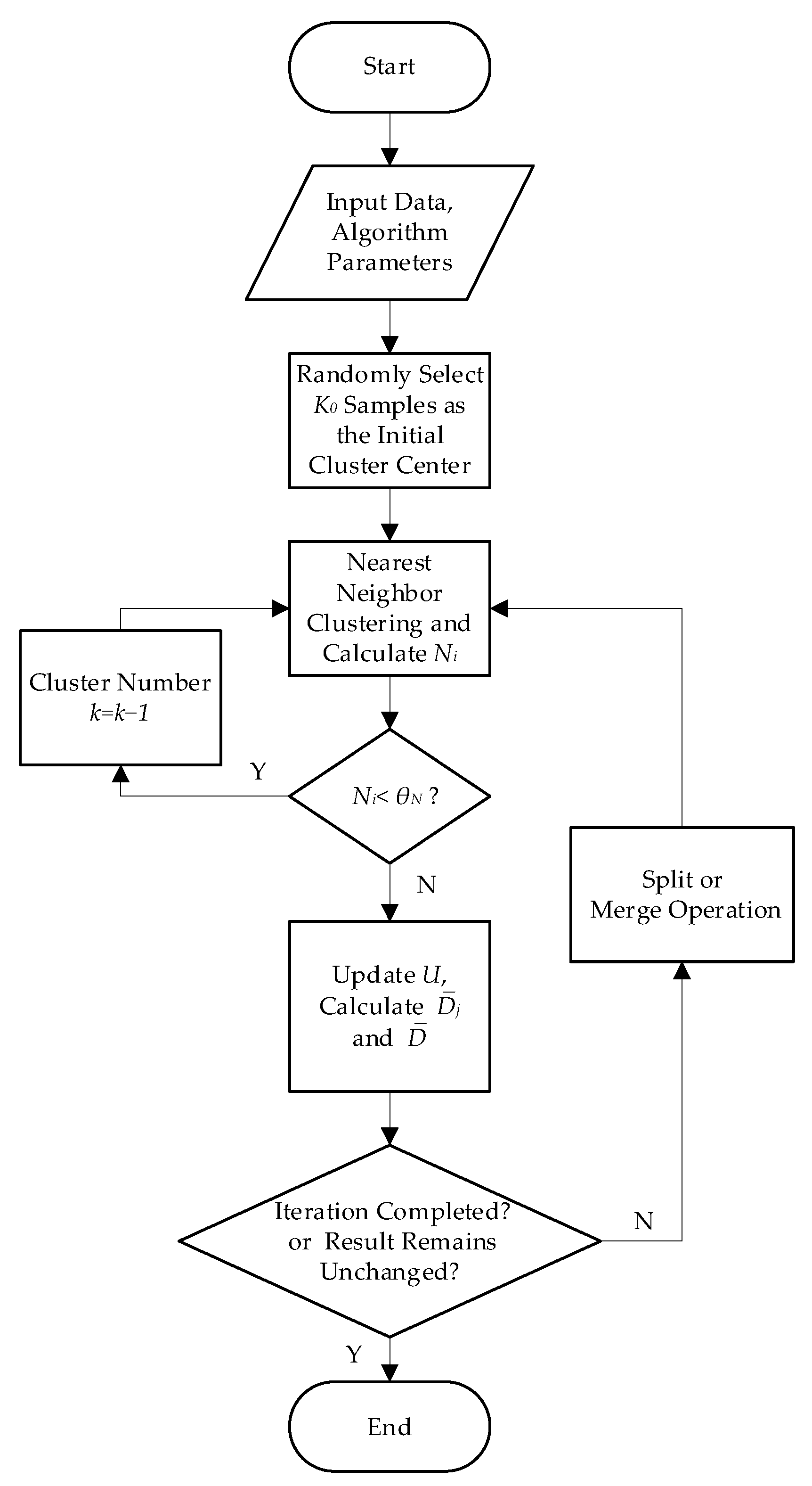
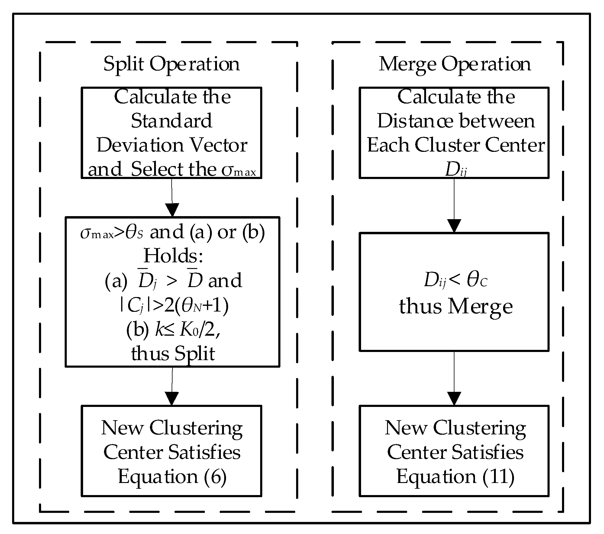
3.2. Cluster Analysis of Historical Scenarios

The ISODATA clustering algorithm is based on the K-means clustering algorithm. Aimed at the problem of how the number of clusters cannot be artificially determined in advance, splitting and merging operations are introduced in the clustering process to achieve dynamical adjustment of the number of clusters to make the clustering results more reliable. Therefore, the ISODATA algorithm is adopted to cluster the historical real wind power and photovoltaic power. The ISODATA clustering algorithm has the following six key parameters.

(1) Expected number of clusters $K_0$: when using the ISODATA clustering algorithm, the number of clusters $K_0$ needs to be given in advance. During the dynamic adjustment process, the number of clusters can be changed within a certain range of $[K_0/2,2K_0]$.

(2) The minimum number of samples ${\theta }_N$ in the cluster: if the number of samples in the cluster after clustering is less than ${\theta }_N$, it cannot be used as a new cluster. During the split operation, it is necessary to ensure that the number of samples in the two subsets after splitting is more than that ${\theta }_N$, otherwise the split fails.

(3) Standard deviation parameter ${\theta }_S$: if the component in the standard deviation vector of a sample in a cluster is greater than ${\theta }_S$, and the number of samples in the subset after splitting is more than ${\theta }_N$, splitting can be performed.

(4) Minimum distance between cluster centers ${\theta }_C$: if the distance between two cluster centers is smaller than ${\theta }_C$, a merge operation is required.

(5) The number of cluster pairs $L$ that are allowed to be merged in each iteration:, the number of cluster pairs to be merged cannot be more than $L$ in each iteration, which is used to limit the number of cluster pairs to be merged.

(6) The maximum number of iterations $I$.

The ISODATA clustering algorithm is shown in Figure 2.

The specific steps are as follows:

(1) Initialize the number of cluster centers $K_0$ and the set of cluster centers $U=\{u_1,u_2,\cdots ,u_n\}$.

(2) For each sample point $x$ in the data set, calculate its distance from all cluster centers and classify it to the nearest cluster center.

(3) Determine whether the number of samples in each cluster $N_i$ is less than ${\theta }_N$, if so, the cluster needs to be discarded, the number of clusters $k=k-1$, and the samples in the cluster are reclassified to the nearest cluster center.

(4) Update the cluster center set C and calculate the mean value of all sample points belonging to the cluster center:

$$u_j=\frac{1}{\left|C_j\right|}{\displaystyle \sum _{x\in C_j}x}$$

(6)

So far, the position of the cluster center is updated.

(5) Calculate the average distance ${\overline{D}}_j$ from the samples in each cluster to the cluster center and the average distance $\overline{D}$ from all samples to the cluster center:

$${\overline{D}}_j=\frac{1}{\left|C_j\right|}{\displaystyle \sum _{x\in C_j}\Vert x-u_j\Vert }$$

(7)

$$\overline{D}=\frac{1}{\left|C_j\right|}{\displaystyle \sum _{j=1}^{\left|C_j\right|}\left|C_j\right|}{\overline{D}}_j$$

(8)

(6) If the clustering result does not change, the iteration is terminated in advance, otherwise, the splitting and merging operations are performed. The detailed process of the splitting and merging operations is shown in Figure 3.

(7) Split clustering: if there is a maximum component in the standard deviation vector of a certain cluster $C_j$ satisfying ${\sigma }_{\max }>{\theta }_S$, and the condition of (a) or (b) holds, the split operation is required.

(a) The current cluster number $k\le K_0/2$

(b) ${\overline{D}}_j>\overline{D}$ and $\left|C_j\right|>2({\theta }_N+1)$

After the split operation, the new cluster center is assumed to be $u_1$ and $u_2$:

$$u_1=u_j+t{[0,\cdots ,{\sigma }_{\max },\cdots ,0]}^T$$

(9)

$$u_2=u_j-t{[0,\cdots ,{\sigma }_{\max },\cdots ,0]}^T$$

(10)

In (9) and (10), $t$ varies in the range of $(0,1]$ and can take 0.5 here.

(8) Merge clustering: if the distance $D_{ij}$ between two cluster centers is smaller than that ${\theta }_C$, then the merge operation can be performed to form a cluster, and the new cluster center is:

$$u=\frac{1}{\left|C_i\right|+\left|C_j\right|}(\left|C_i\right|u_i+\left|C_j\right|u_j)$$

(11)

(9) Return to step (3) until the clustering result remains unchanged or the maximum number of iterations is reached, and the final cluster center set $U$ and clustering result are returned.

3.3. Determination of Day-Ahead Consumption Service Reserve Demand

According to the time scale division standard of reserve resources in Table 1, three structural elements with corresponding time scale characteristics are designed. The time scales are divided into four levels, which are 10 min, 30 min, 60 min, and over 60 min, and the disc-shaped structural elements with heights of 5 MW, 10 MW, and 20 MW are selected to carry out three-level filtering on the forecast error curve sample with four fluctuation components corresponding to the different time scales extracted. In this way, the multi-time-scale fluctuation characteristics of the forecast error curve are drawn out, including fluctuation components within 10 min, 10–30 min, 30–60 min, and over 60 min.

For all levels of fluctuation components of all historical forecast error sample curves in the same scenario set, the absolute amplitudes of the positive and negative envelopes of the fluctuation components are extracted by using the cubic spline interpolation method. According to the absolute values of the envelopes, the hierarchical consumption service reserve demand for each period in the matched scenario under a certain confidence level is formulated as follows:

$$\mathrm{Pr}\left(a{u}_{i,j}(t)<N{U}_{j,t}\right)=\beta \forall i\in [1,n],t\in [1,T]$$

(12)

$$\mathrm{Pr}\left(a{d}_{i,j}(t)<N{D}_{j,t}\right)=\beta \forall i\in [1,n],t\in [1,T]$$

(13)

where, $T$ is the total dispatch period, $n$ is the total number of samples in a certain scenario, and $\mathrm{Pr}(•)$ is the probability distribution function of the absolute value of the envelope. $j$ is the reserve level, $j=1,2,3,4$, and $\beta$ is the confidence level. $a{u}_{i,j}(t)$ and $a{d}_{i,j}(t)$ are the absolute values of the positive and negative envelopes of the level fluctuations of any sample i in the period t in this scenario. $N{U}_{j,t}$ and $N{D}_{j,t}$ are the upward and downward reserve demand for level 1 of the t dispatch period.

4. Discussion

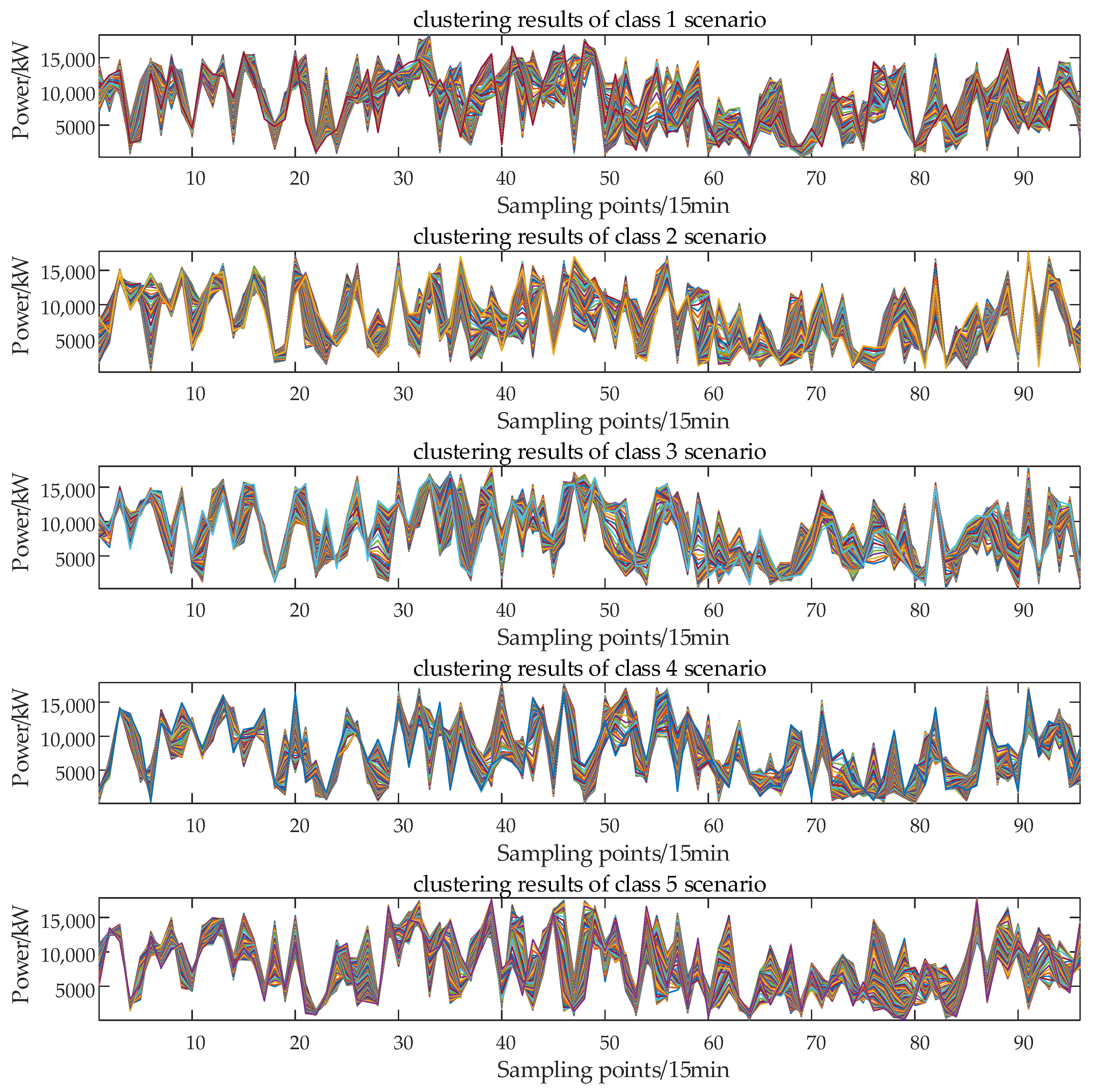
4.1. Scenario Clustering Results

Taking the total output power of all the wind farms in north China as an example, the ISODATA clustering is performed on its actual historical output power in 2022. The advantages of the algorithm are further verified. We set the ISODATA algorithm parameters $K_0=8$, ${\theta }_N=10$, ${\theta }_S=0.15$, ${\theta }_C=2$, $L=1$, $I=100$. The real output of wind power is clustered, and the results of each scenario are shown in Figure 4. The initial number of clusters is eight categories, and after the splitting and merging operations in the iterative process, the algorithm finds the best cluster number of five.

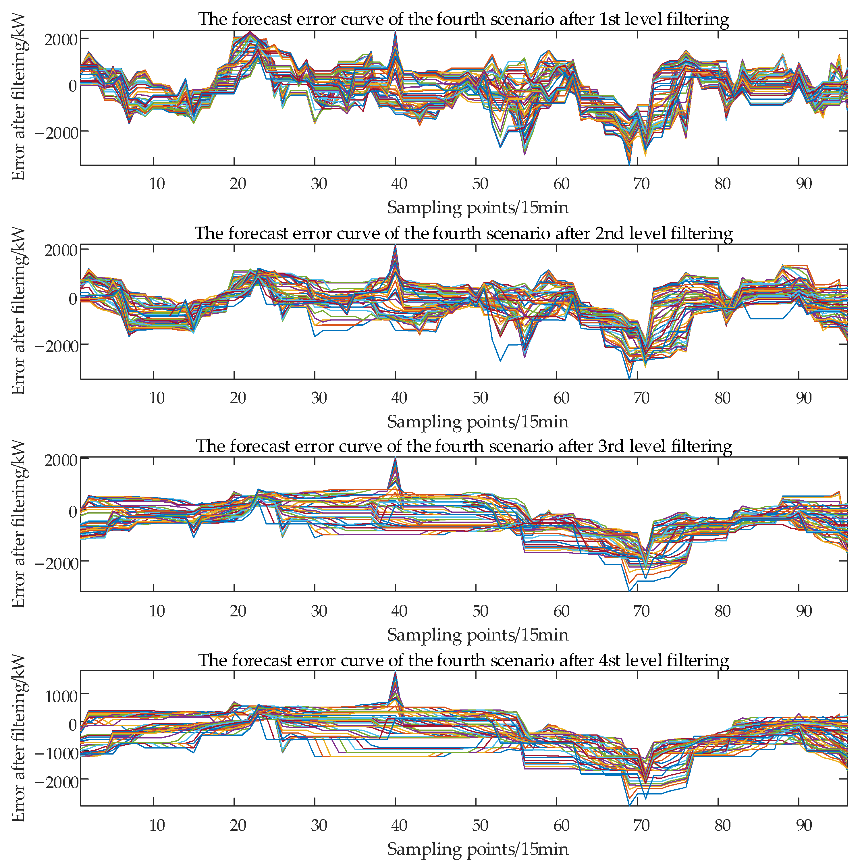
4.2. Forecast Error Decomposition Results

The power forecast data on 1 December 2022 were selected as the example day to be analyzed for scenario matching. Firstly, the distance between it and the cluster center of each clustering scenario is calculated, and then the scenario of the wind power forecast data on that day was obtained as the fourth clustering scenario. Based on the mathematical morphology filter, the corresponding multi-time-scale decomposition is performed on the error sample curves of all net load forecasts in different scenarios. According to the time scale classification standard of reserve resources at all levels, disc-shaped structural elements with time scales of 10 min, 30 min, and 60 min and heights of 5 MW, 10 MW, and 20 MW were, respectively, selected in each scenario. The error sample curve is decomposed on multiple time scales. Among them, the decomposition results of the forecast error in the fourth type of clustering scenario are shown in Figure 5.

4.3. The Dynamic Assessment Results of Consumption Service Reserve Demand

According to the information on day-ahead forecast power data, the matched scenario is the fourth scenario. For the forecast error curve of the fourth scenario, the four-level fluctuation component is obtained through three-level filtering. Then, the positive fluctuation maximum value sequence and the negative fluctuation minimum value sequence of the decomposition results obtained by morphology are, respectively, extracted by cubic spline interpolation. The hierarchical reserve demand of the fourth scenario is calculated based on the envelope extraction results when the confidence level is 95%, as shown in Figure 6. The red line is the assessment result of the up-reserve demand, while the blue line represents the down-reserve demand.

5. Conclusions

With the goal of achieving safe and economical operation of the power system with high penetration of renewable energy power, this paper puts forward a hierarchical and dynamic assessment method for consumption service reserve demand which is designed to cope with uncertain power in real-time dispatch. The dynamic assessment method is proposed based on the combination methods of the ISODATA clustering algorithm and the morphological filter decomposition algorithm; thus, it effectively reduces the redundancy of reserve and improves the economy of power systems. By incorporating the ISODATA clustering algorithm, an iterative solution method for cluster number is established to construct the typical scenarios of wind power. Moreover, the morphology filter is adopted to decompose the historical forecast error of the matched typical scenario and realize the multi-time-scale extraction of the uncertainty degree.

References

1. Zhuo, Z.; Zhang, N.; Xie, X.; Li, H.; Kang, C. Key Technologies and Developing Challenges of Power System with High Proportion of Renewable Energy. Autom. Electr. Power Syst. 2021, 45, 171–191. [Google Scholar]
2. Xia, S.; Song, L.; Wu, Y.; Ma, Z.; Jing, J.; Ding, Z.; Li, G. An Integrated LHS–CD Approach for Power System Security Risk Assessment with Consideration of Source–Network and Load Uncertainties. Processes 2019, 7, 900. [Google Scholar] [CrossRef] [Green Version]
3. Ullah, Z.; Arshad; Hassanin, H.; Cugley, J.; Alawi, M.A. Planning, Operation, and Design of Market-Based Virtual Power Plant Considering Uncertainty. Energies 2022, 15, 7290. [Google Scholar] [CrossRef]
4. Falvo, M.C.; Panella, S.; Caprabianca, M.; Quaglia, F. A Review on Unit Commitment Algorithms for the Italian Electricity Market. Energies 2022, 15, 18. [Google Scholar] [CrossRef]
5. Lee, T.-Y. Optimal Spinning Reserve for a Wind-Thermal Power System Using EIPSO. IEEE Trans. Power Syst. 2007, 22, 1612–1621. [Google Scholar] [CrossRef]
6. Morales, J.M.; Conejo, A.J.; Perez-Ruiz, J. Economic Valuation of Reserves in Power Systems With High Penetration of Wind Power. IEEE Trans. Power Syst. 2009, 24, 900–910. [Google Scholar] [CrossRef]
7. Yang, H.-T.; Wu, Y.-S.; Liao, J.-T. Economic Dispatch and Frequency-Regulation Reserve Capacity Integrated Optimization for High-Penetration Renewable Smart Grids. In Proceedings of the 2019 IEEE Innovative Smart Grid Technologies—Asia (ISGT Asia), Chengdu, China, 21–24 May 2019; pp. 2980–2985. [Google Scholar]
8. Cheng, J. Capacity Assessment of Agricultural Irrigation Load Participating in Operating Reserve of Power System. In Proceedings of the 2021 IEEE Sustainable Power and Energy Conference (iSPEC), Nanjing, China, 23–25 December 2021; pp. 2511–2517. [Google Scholar]
9. Zhang, D.; Xu, J.; Sun, Y.; Liao, S.; Ke, D. Day-ahead dynamic estimation and optimization of reserve in power systems with wind power. Power Syst. Technol. 2019, 43, 3252–3260. [Google Scholar] [CrossRef]
10. Wang, D.; Chen, Z.; Tu, M.; Yang, Z.; Ding, Q. Reserve capacity calculation considering large-scale wind power integration. Autom. Electr. Power Syst. 2012, 36, 24–28. [Google Scholar]
11. Wu, S.; Chi, F.; Ye, X.; Kuang, L.; Wang, Z.; Wen, Y. Probabilistic Dynamic Assessment for Operating Reserve Requirements of Power System with High Penetrated Renewables. Power Constr. 2023, 44, 126–134. [Google Scholar]
12. Gong, Y.; Jiang, Q.; Baldick, R. Ramp Event Forecast Based Wind Power Ramp Control With Energy Storage System. IEEE Trans. Power Syst. 2016, 31, 1831–1844. [Google Scholar] [CrossRef]
13. Bhavsar, S.; Pitchumani, R.; Ortega-Vazquez, M.A. A Reforecast-Based Dynamic Reserve Estimation for Variable Renewable Generation and Demand Uncertainty. Electr. Power Syst. Res. 2022, 211, 108157. [Google Scholar] [CrossRef]
14. Qian, K.; Wang, X.; Yuan, Y. Research on Regional Short-Term Power Load Forecast Model and Case Analysis. Processes 2021, 9, 1617. [Google Scholar] [CrossRef]
15. Li, Y.; Bai, X.; Meng, J.; Zheng, L. Multi-Level Refined Power System Operation Mode Analysis: A Data-Driven Approach. IET Gener. Transm. Distrib. 2022, 16, 2654–2680. [Google Scholar] [CrossRef]
16. Zhang, X.; Chen, Y.; Wang, Y.; Ding, R.; Zheng, Y.; Wang, Y.; Zha, X.; Cheng, X. Reactive Voltage Partitioning Method for the Power Grid With Comprehensive Consideration of Wind Power Fluctuation and Uncertainty. IEEE Access 2020, 8, 124514–124525. [Google Scholar] [CrossRef]
17. Lin, Z.; Chen, Z.; Qu, C.; Guo, Y.; Liu, J.; Wu, Q. A Hierarchical Clustering-Based Optimization Strategy for Active Power Dispatch of Large-Scale Wind Farm. Int. J. Electr. Power Energy Syst. 2020, 121, 106155. [Google Scholar] [CrossRef]
18. Lin, S.; Li, F.; Tian, E.; Fu, Y.; Li, D. Clustering Load Profiles for Demand Response Applications. IEEE Trans. Smart Grid 2019, 10, 1599–1607. [Google Scholar] [CrossRef]
19. Li, Z.; Yu, X. Power Load Curve Clustering Based on ISODATA. In Proceedings of the 2022 IEEE 7th International Conference on Smart Cloud (SmartCloud), Shanghai, China, 8–10 October 2022; pp. 104–108. [Google Scholar]
20. Xie, F.; Liang, K.; Wu, W.; Hong, W.; Qiu, C. Multiple Harmonic Suppression Method for Induction Motor Based on Hybrid Morphological Filters. IEEE Access 2019, 7, 151618–151627. [Google Scholar] [CrossRef]
21. Wang, X. Electric network security setup in electricity market environment. Power Syst. Technol. 2004, 7–13. [Google Scholar] [CrossRef]
Figure 1. Several common structural elements.
Energies 16 05979 g001
Figure 2. Flow chart of the ISODATA clustering algorithm.
Energies 16 05979 g002
Figure 3. Flow chart of merge operation and split operation in the ISODATA clustering algorithm.
Energies 16 05979 g003
Figure 4. Clustering scenarios of historical wind power.
Energies 16 05979 g004
Figure 5. Decomposition results of forecast error of scenario 4.
Energies 16 05979 g005
Figure 6. Dynamic assessment results of reserve demand at all levels.
Energies 16 05979 g006