Advancing Sustainable Decomposition of Biomass Tar Model Compound: Machine Learning, Kinetic Modeling, and Experimental Investigation in a Non-Thermal Plasma Dielectric Barrier Discharge Reactor

Abstract

This study examines the sustainable decomposition reactions of benzene using non-thermal plasma (NTP) in a dielectric barrier discharge (DBD) reactor. The aim is to investigate the factors influencing benzene decomposition process, including input power, concentration, and residence time, through kinetic modeling, reactor performance assessment, and machine learning techniques. To further enhance the understanding and modeling of the decomposition process, the researchers determine the apparent decomposition rate constant, which is incorporated into a kinetic model using a novel theoretical plug flow reactor analogy model. The resulting reactor model is simulated using the ODE45 solver in MATLAB, with advanced machine learning algorithms and performance metrics such as RMSE, MSE, and MAE employed to improve accuracy. The analysis reveals that higher input discharge power and longer residence time result in increased tar analogue compound (TAC) decomposition. The results indicate that higher input discharge power leads to a significant improvement in the TAC decomposition rate, reaching 82.9%. The machine learning model achieved very good agreement with the experiments, showing a decomposition rate of 83.01%. The model flagged potential hotspots at 15% and 25% of the reactor’s length, which is important in terms of engineering design of scaled-up reactors.

1. Introduction

Biomass processing is a dual approach for handling biowaste [1,2] and energy production simultaneously [3,4]. It is a predominant resource in thermochemical processes, i.e., gasification and pyrolysis, to simultaneously produce heat and clean energy [5,6,7,8]. Typically, producer gas consists of H₂, CO, CO₂, CH₄, as well as other hydrocarbons, and N₂ if air is used as a gasifying agent [9,10,11,12]. Among the variety of hydrocarbons produced during gasification, one should distinguish tars, which are problematic in terms of downstream processing of the producer gas [13,14,15,16].

Different classifications of tars exist, with the most common being the ECN classification. According to this classification, all tars undetectable by gas chromatography (heaviest tars) belong to class 1, heterocyclic compounds (e.g., phenol, pyridine, cresol) belong to class 2, aromatic compounds with one ring (e.g., xylene, styrene, toluene) belong to class 3, light polyaromatic hydrocarbons with two to three rings (e.g., naphthalene, biphenyl, acenaphthylene, phenanthrene, anthracene) belong to class 4, and heavy polyaromatic hydrocarbons with more than three rings (e.g., fluoranthene, pyrene, chrysene) belong to class 5 [17].

Tar can be removed by primary and secondary methods [18,19,20,21]. In primary methods, tars are removed within the gasifier, while secondary methods involve post-gasifier treatment [22,23,24]. Thermal cracking, which is one of the methods of decomposition of tars, requires a relatively high reaction temperature of 800 °C [25], which leads to large energy consumption [24,26]. Deficiencies in the primary methods and conventional technologies i.e., thermal cracking, oxidation, and adsorption, lead to intensive research on novel methods of tar removal.

Non-thermal plasma (NTP) technologies are energy-efficient and produce the required results for the removal of volatile organic compounds (VOC), organic solvents, and chlorofluorocarbon, as well as other pollutants present in exhaust streams, and industrial waste gases [18,24]. “Plasma” term refers to partial or full ionization of available gas for ions and radical propagation from atoms and molecules by inducing electrons [27,28]. Plasma is categorized by temperature ranges [28]. In thermal plasma, all the substituents have the same temperature, whereas in NTP no temperature equilibrium exists between kinetically energized excited electrons and constituent gaseous or pollutant particles such as ions, atoms, radicals, etc. [28]. NTP reactors are characterized on an electrical discharge basis named dielectric barrier discharge (DBD), electron beam irradiations, glow discharge, and pulse corona discharge [28]. Plasma discharge reactors are convenient due to instantaneous electron temperature and reactivity because of available ions, radicals, and pulses [29]. The electron beam process is quite efficient in the removal of emissive pollutants, while corona and dielectric discharges are suitable for domestic and industrial applications due to the variable reactor length and streamer frequency [29]. DBD reactors can be used to purify gas, reduce tar contents, and increase the quality of the processed gases [29]. They usually have greater selectivity and optimum operating conditions and operate at room temperature [29]. Radicals produced are short-lived and have good removal efficiency [30]. The major energy input of the NTP reactor goes into the production of an electron rather than for heating purposes. Firstly, electron generation starts by exciting gas molecules and direct collision with atoms, producing radicals such as O•, OH⁻¹, H•, etc. This leads to multiple reaction paths and eventually causes the desired decomposition of reactants. In DBD reactors (see Figure 1), the amount of pollutant for decomposition, the energy cost of toxic molecule removal, and energy efficiency are the main parameters for consideration. These factors are based on reaction rates, electrode configurations, reactor packing, and the input energy transfer from the power source with available reactor length [31].

Among all the VOCs, benzene is the least reactive and has a slower reaction rate constant [32]. Although current tar definition excludes benzene, it is still used as a model compound in many studies on plasma decomposition of tars [30,33,34,35,36]. The reason for this is the aforementioned stability and low reactivity. Furthermore, benzene is a border compound, defining tars, and many of the heavier compounds classified as tars contain multiple benzene rings [17].

Plasma modeling and reaction engineering is complex and confined to a generalized model, confining major properties of physical and chemical nature [37]. In recent years, machine learning (ML) has attracted significant attention as a powerful tool for a wide variety of chemical process optimization and online active prediction. ML has been extensively used in environmental and pollution-oriented processes due to greater error reduction quality. Earlier researchers employed conventional artificial neural network (ANN) methods for the complex plasma conversion of syngas and methane. In plasma-centered studies, different ML algorithms are used according to their applicability and drawbacks [38,39,40]. ML algorithms are shortlists based on performance and solutions of process in industry vital for nonlinear and complex systems. An increase in the number of variables entails a significant complication in calculations and reliable result forecasting, due to labeled and unlabeled datasets, missing values, random errors, bad points, data distributions, etc.

Liu et al. [41] highlighted an ML application for gas conversion for environmental pollutant control in a plasma environment through three-layer back propagation ANN for studying the non-oxidative reaction conversion of methane molecules. In plasma process modeling, discharge power is the most significant parameter for conversion, while the least significant factor is excitation frequency [42]. Chang’s ANN model is a four-experimental-parameter study for better understating the effect on toluene removal. Parameters were input discharge power, initial concentration, flow rate, and relative humidity [43].

The novelty of this study is the application of machine learning techniques for modeling of benzene conversion in a DBD plasma reactor.

Figure 1. Discharge barrier NTP technology characteristics for gasification tar reduction, based on [44].

Figure 1. Discharge barrier NTP technology characteristics for gasification tar reduction, based on [44].

2. Materials and Methods

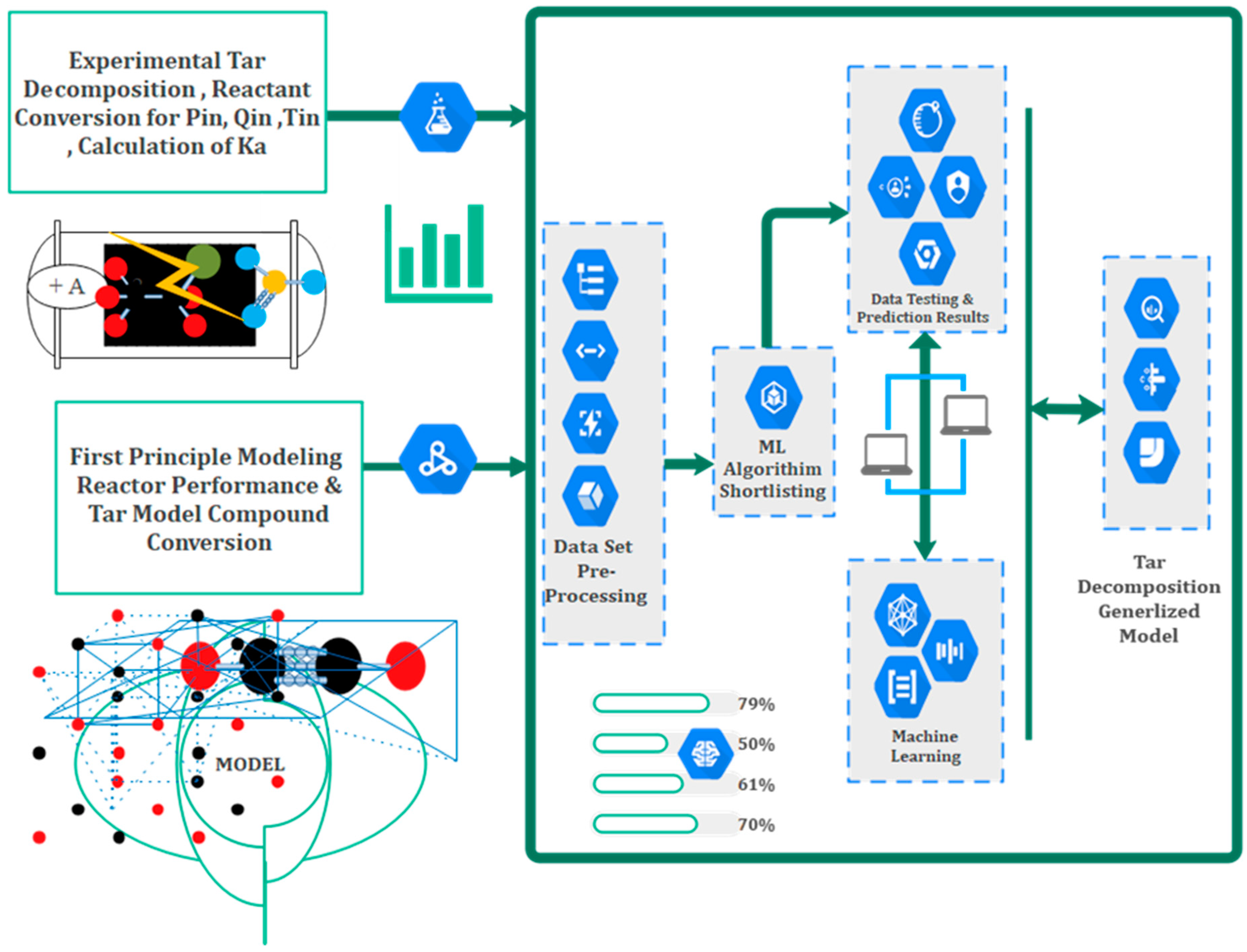
2.1. Non-Thermal Plasma Kinetic Modeling with Machine Learning Algorithms

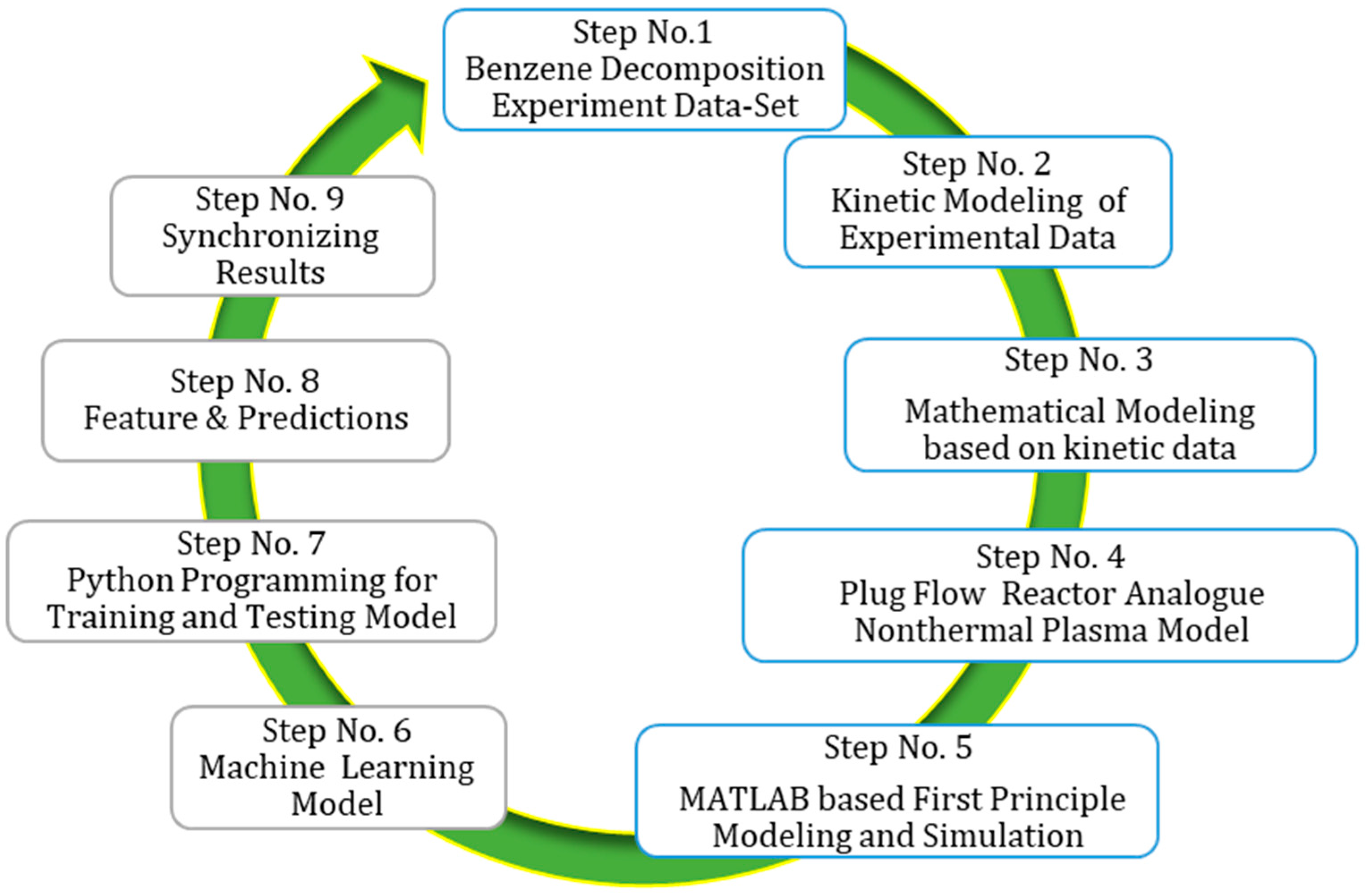
Plasma modeling systems degenerate into smaller and general global models depending on variables of interest. These usually comprise three methods: kinetic, fluid, and hybrid plasma modeling. Kinetic modeling becomes tedious owing to high computation and difficulty in chemistries of reaction and multiple species propagations within a duration of nanoseconds.

Supervised learning deals with labeled datasets and has two processes for regression and classification. Unsupervised learning mainly uses unlabeled data with no idea about the type of results and is divided into clustering and dimensionality reductions. Semisupervised learning is a hybrid and lies between supervised and supervised learning combining labeled and unlabeled data. Reinforcement learning has no training datasets and utilizes a reward-based scheme. The framework of the research performed is shown in Figure 1. Through the integration of kinetic-based modeling, simulation of experimental data, and the tar analogue model, we embarked on a transformative journey. This joint endeavor aimed to unravel the intricate process parameters and multifaceted reaction complexities inherent in non-equilibrium plasma conditions. By delving deep into the depths of understanding, a profound insight into plasma chemistry is uncovered, igniting a pathway for further exploration.

One of the noteworthy outcomes of this advanced research is aligning experimental findings with modeling and knowledge-driven results, for a comprehensive understanding of plasma dynamics is obtained. It is important to acknowledge that although there may be variations between the experimental and reactor models, these deviations are primarily due to streamlined assumptions made for efficient calculations.

In this compelling narrative, machine learning emerges as a game-changer. Serving as an invaluable black box tool, it seamlessly integrates with the kinetic and reactor models, reducing statistical errors and bolstering accuracy. This triumvirate approach between kinetic-based modeling, reactor simulation, and machine learning sets the stage for a paradigm shift in NTP reaction chemistry, decomposition kinetics, and result validation. The culmination of these novel insights fuels an unyielding passion for plasma studies and paves the way for ingenious solutions to intricate engineering problems. Given the urgency of the times, the commercialization of an economically viable tar removal process assumes paramount importance. Not only does it offer a sustainable solution but it also creates an environment conducive to biomass gasification-based energy production applications.

2.2. Working Cycle

This paper focuses on proposing and shortlisting a working cycle for the process industry connecting experimentation to a data-driven process model. The goal is to address the challenges posed by an increased number of variables, such as labeled and unlabeled datasets, missing values, random errors, and data distribution, in order to achieve reliable result forecasting. The detailed working cycle is presented in Figure 2. The proposed working cycle consists of several key steps. Step 1 involves obtaining experimentation results to analyze the decomposition of benzene. Step 2 entails the kinetics of hypothetical ideal plug flow reactor performance, which are then compared against experimental results from the DBD reactor. In Step 3, comparison and synchronization of the experimental and modeling results are performed to reduce errors and lay the foundation for future scale-up studies.

The subsequent steps involve the application of various methodologies and tools. Step 4 focuses on the development of a plug flow reactor analogue model for non-thermal plasma. Step 5 utilizes MATLAB for first-principle modeling and simulation. Step 6 incorporates machine learning models to enhance the analysis. Step 7 involves using Python programming for training and testing the models. Step 8 revolves around extracting features and making predictions based on the trained models. Finally, in Step 9, the results are synchronized and evaluated. This comprehensive working cycle aims to provide valuable insights into the complex dynamics of the process industry, bridging the gap between experimentation and modeling for improved accuracy and scalability.

2.3. Experimental Methodology and Materials

In this study, a dataset was obtained from an experiment [36] using a coaxial NTP single-stage DBD reactor to decompose benzene, a tar model compound. The experimental setup involved a plasma reactor with a plasma zone between quartz tubes, operating at a frequency of 20 kHz and a voltage of 20 kV. The power of the DBD reactor ranged from 5 to 40 W, determined by the length of the outer electrode at ambient temperature conditions. Analysis of the plasma reaction’s end products was conducted using a gas chromatograph (GC), i.e., a Varian 450-GC equipped with flame ionization and thermal conductivity detectors. The DBD reactor’s external electrode was composed of stainless steel and wrapped with a quartz tube. Discharge power was regulated using a Variac AC transformer and measured with an energy meter. Gas flow was controlled by computer-controlled mass flow controllers, with a fixed flow rate of 40 mL/min for methane and nitrogen. Product composition was analyzed using the Varian 450-GC with flame ionization and thermal conductivity detectors. The same experimental conditions were employed for kinetic modeling, reactor assessment, and machine learning.

Total benzene removal efficiency and specific input energy are defined as:

$$Benzene Removal Efficiency\left(d_b\right)=\frac{C_6{H}_{6 in}-C_6{H}_{6 out}}{C_6{H}_{6 in}}\times 100$$

(1)

$$Specific Input Energy\left(SIE\frac{Joule}{Liter}\right)=\frac{Power\left(Joule/Second\right)}{Total gas flow rate\left(\frac{Liter}{Second}\right)}$$

(2)

Faisal et al. [36] reveals clear trends regarding the effects of input power, concentration of the tar analogue compound, and residence time. Increasing the input power results in higher decomposition of benzene. This correlation can be attributed to the generation of high-energy electrons and reactive species at higher plasma input power. The trend shows a gradual rise in benzene decomposition as the power input varies from 5 W to 40 W, reaching 82.9% at 40 W for a constant residence time of 2.86 s and a concentration of 36 mg/Nm³. The R² value of 0.856 suggests a significant influence of input power on benzene decomposition, as shown in Figure 3a.

The theoretical understanding indicates that the increase in decomposition is due to the presence of high-energy electrons generated at high plasma input power. These electrons collide with CH₄, generating reactive species such as radicals, excited molecules, and ions, which actively contribute to the decomposition of benzene. The reactions involved include the formation of reactive species and the production of lower hydrocarbons by breaking the aromatic ring [36,45]. The high-energy electrons also decompose the carrier gas, CH₄, resulting in the formation of reactive radicals such as CH₃ and H. These radicals directly break aromatic rings, leading to the generation of lower hydrocarbons. Radical termination reactions can occur, producing CH₄ through the combination of CH₃ and H radicals. Agglomeration reactions may also take place within this mechanism [36,46].

Initiation:

CH₄ + e⁻ --------------------------- > CH₃· + H⁺ + e⁻

Propagation:

C₆H₆ + e⁻ --------------------------- > C₆H₅ + e⁻

C₆H₆ + H⁺ --------------------------- > C₆H₅ + H₂

Termination:

C₆H₅ + Energetic Species --------------------------- > Solid Residue + Lower Hydrocarbon

The results demonstrate that the decomposition of CH₄ increases with higher input power, attributed to the presence of reactive species and energetic electrons. These radicals contribute to the decomposition of methane into valuable hydrocarbons and hydrogen through combination and agglomeration reactions. Regarding the effect of residence time on benzene removal, increasing residence time leads to higher removal efficiency. The removal of benzene shows a linear increase from 37.5% to 68.8% as residence time increases to 2.86 s at a power input of 20 W and a concentration of 36 g/Nm³. This trend suggests that longer exposure to the plasma discharge zone enhances collisions between the tar model compound and active species, resulting in increased benzene removal, as shown in Figure 3b [36,38,47,48].

The R² value of 0.996 indicates a good likelihood of dependence on both residence time and power input simultaneously. On the other hand, the removal of benzene decreases as the concentration of the tar analogue compound increases at a constant power input of 15 W and residence time of 2.86 s, as shown in Figure 3c. The higher concentration of benzene leads to a greater number of benzene molecules in the discharge zone, increasing the probability of unconverted benzene escaping and reducing overall removal efficiency. This trend is observed regardless of the nature of the carrier gas, indicating that the impact of concentration on removal efficiency and energy utilization remains consistent [36,39].

These findings provide valuable insights for understanding and predicting the system’s behavior and can be utilized to optimize process parameters. Kinetic modeling, simulation, and machine learning studies can incorporate the observed reactions and trends to better understand mechanisms and predict behavior under different conditions, as shown in Figure 4. This information is particularly useful in plasma chemistry and catalysis research, aiding in reactor design, process optimization, and catalyst development.

Further analysis and consideration of factors such as flow rate and concentration may be necessary for a comprehensive understanding and accurate modeling of the relationship between input power and benzene decomposition. Nonetheless, the experimental findings and trends offer valuable guidance for kinetic modeling, simulation, and machine learning studies, advancing research in plasma chemistry and catalysis.

2.4. Kinetic Modeling and Reactor Performance Assessment

Three types of kinetic models are present in the literature for tar removal kinetics. Kinetic modeling has been widely used for the abatement of emissions of pollutants [49]. Studies have been based on the time-dependence characteristics of input power, feed flow rate, gas hourly space velocity, instantaneous conversion, reactor-based radical generation, and energy efficiency. The kinetic behavior of tar removal within a plasma reactor accounts for the rate constant, reaction order, activation energy, and radical propagation [50,51]. Best-fit line, sum of square of error, standard deviation, and numerical methods were used for simulation and conversion of naphthalene with nitrogen and carrier gas mixtures for 350 elementary and 77 component species in RADICAL software. It defined a new self-consistent chemical kinetic model based on G values [52]. The Chemkin software Plug Flow module simulates a 257 set of reactions and compares the modeling and bench-scale experimentation results. Global kinetics are proposed. Toluene and benzene show zero- and first-order kinetics, respectively. Benzene gives the least specific energy density in comparison to toluene and styrene. The overall reaction rate constant compares systems and predicts the removal rate of VOCs, especially in NTP reactors [45].

In our research model, a global kinetic model for removal of a tar model compound from a synthetic gasifier output gas stream shall be developed and extended, as a suggested principle discussed in the literature [53,54]. Reaction conditions are room temperature plasma within single-stage dielectric barrier discharge reactor geometry with varying operational conditions with the help of computer-aided tools such as MATLAB R.21, Python 3.8 Anaconda Version, Design Expert 12 for modeling and simulation studies of a kinetic model for the DBD reactor as empirical modules for studying decomposition reactions. Reactor modeling investigates different parameters, such as input power, removal rate, and residence time within the DBD reactor. Validating a plasma kinetic behavior model at inputs (power and process conditions) and reactor performance evaluation (reactant decomposition) should be conducted against the experimental setup in present and future scenarios for scale-up studies. Kinetic theory is the basis for complex reactions and aims to develop a comprehensive and reliable simplified kinetic reaction model for the decomposition of benzene, serving as the tar analogue compound.

Figure 4 shows the extended methodology employed based on a novel strategy synergizing experimental data with kinetics, modeling and machine learning studies. It involves the utilization of both integral and differentiation methods in the MATLAB environment. Extensive concentration-based investigations reveal that the second step of the reaction is rate-determining, primarily due to its higher concentration. To facilitate the modeling process, several key assumptions are made. Firstly, the system is assumed to be in a quasi-steady state, ensuring the constancy of reaction rates over time.

Secondly, the mixture is considered heterogeneous, acknowledging the presence of multiple phases. The system is assumed to operate under ideal plug flow reactor conditions, which ensure uniform flow and minimal mixing. The process is assumed to occur under isothermal conditions, maintaining a constant temperature throughout the reaction. Lastly, it is assumed that the energy density of the system remains constant during the entire reaction process. These assumptions, in conjunction with a combination of mathematical techniques, allow for the development of a simplified kinetic reaction model that enhances our understanding of the benzene decomposition process [36] for experimental work and overcomes the data noise and unavoidable errors during experimentation of the plasma process.

Five additional assumptions are considered to maintain a reliable and efficient computation of differential equations in one dimension. The ideal plug flow reactor exhibits similar reactant conversion for decomposition characteristics, as observed in popular software, such as Chemkin and Comsol. NTP reactors, which are less affected by temperature variations, perform well within lower temperature ranges. Lastly, the assumption of constant energy density is justified by the uniform nature of discharge plasma along the length of the reactor.

3. Results

3.1. Rate-Constant Calculation

Plasma kinetic modeling simulates the general reaction sequence and mechanism for the calculation of the rate constant. It commences with initiation reactions, and the second step is the decomposition reaction that involves the reaction of radical interaction with benzene molecules. The reaction sequence terminates with the formation of yellow solid formation, indicating the decomposition of benzene compounds into multiple- and single-chain carbon compounds.

Based on the reaction mechanism rate of decomposition of benzene, a tar analogue compound is dependent on the initiation reaction and decomposition step. The initiating reaction amount of available concentration of benzene and carrier mixture is directly under the power input as influx. It results in radical propagation due to high energy electrons and decomposes the available benzene. Hence, the decomposition step is the rate-determining step and calculates the rate constant for the global macro-kinetic model under uniform energy density conditions. Radical concentration is difficult to account for and accurately measured, and hence the mechanistic kinetic theory is the basis for the rate-constant calculations.

Initiation:

Gas (Benzene + Synthetic Mixture Gas) ------ > Radical (R)

$$R1=K_1\left(\frac{P_{in}}{Vr}\right)$$

(3)

Decomposition step:

Benzene --------- > Intermediates (Y) + Lighter Hydrocarbon Compounds

$${ R}_2=K_2\ast C_a$$

(4)

Completing Reaction Step:

Y + R ------ > Solid Carbons + Light Hydrocarbons + Complex Products

Based on the reaction mechanism rate of decomposition of benzene, a tar analogue compound is dependent on the abovementioned Equations (3) and (4). For the initiation reaction, the amount of available benzene and carrier mixture depends directly on the power input. It results in radical propagation due to high energy electrons and decomposes the available benzene. Hence, the decomposition step is the rate-determining step and calculates the rate constant for the global macro-kinetic model under uniform energy density conditions. Radical concentration is difficult to account for and accurately measure; hence, the mechanistic kinetic theory is the basis for the rate-constant calculations. An ideally 1-D plug flow reactor with quasi-steady-state plasma is considered and explicitly expressed as mainly used in literature as an alternative to an NTP DBD reactor as well as in such commercial software as Chemkin design and model equations.

$$R_a=-\frac{d{C}_a}{dt}=R_1\ast R_2$$

(5)

R₁ is the effectiveness of the available active species that react with benzene at a certain input power P_in across discharge reactor length for the model compound concentration C_a, while K₁ is the radical production constant and K₂ is the resultant decomposition of benzene for the reaction time for carrier gas flow rate (Q_in) defining the specific input energy (SIE). The product of K₁ and K₂ is the apparent benzene decomposition rate constant (K_d).

$$R_a=-\frac{d{C}_a}{dt}=K_1\left(\frac{P_{in}}{Vr}\right)\ast K_2\ast C_a$$

(6)

$${Decomposition Constatnt K}_{d }=K_1\ast K_2$$

(7)

$$Reaction time t=\frac{V_r}{Q}$$

(8)

$$-Ln\left(\frac{C_{out}}{C_{in}}\right)=K_d\ast \frac{P}{Q}$$

(9)

$$-Ln\left({1-X}_A\right)=K_d\ast \frac{P}{Q}$$

(10)

$$SIE=\left(\frac{P_{in}}{Q}\right)$$

(11)

$$-Ln\left({1-X}_A\right)=K_d\ast SIE$$

(12)

A dual technique for calculating the apparent decomposition constant is using the regression technique by analyzing the experimentation results using Equation (12). The other method is the differentiation method for a model in MATLAB R-21 for dC_a/dt Vs t. The reaction rate constant by the regression technique is 0.040 (L/kJ), as shown in Figure 5. The differentiation method deduces the order of reaction of n = 1, and the rate constant is the same as the earlier decomposition rate constant.

The apparent rate constant for the decomposition of benzene, obtained through the regression technique as 0.040 (L/kJ), represents the rate at which benzene molecules undergo decomposition under the given experimental conditions, and gives a better R² value of 0.99 in comparison to 0.96 obtained in the experiment of Faisal et al. [36]. This value indicates the rate of the overall reaction and reflects the effectiveness of the reaction in converting benzene into the desired products. It signifies the relationship between the concentration of benzene (in moles per liter) and the input energy (in kilojoules). It indicates the change in concentration of benzene per unit time, per unit concentration, and per unit input energy. The obtained value of 0.040 (L/kJ) represents the best estimate of the rate constant based on the available experimental data. The value of the rate constant can vary depending on the specific experimental conditions. Different experimental setups and conditions can result in different apparent rate constants, as they influence the reaction kinetics and increase the noise, as highlighted in Figure 3a–c and value of R². The apparent rate constant serves as a crucial parameter in understanding and characterizing the kinetics of the benzene decomposition reaction. It provides information about the speed and efficiency of the reaction and can be used to model and predict the behavior of the reaction under different conditions.

3.2. Reactor Mathematical Model for Performance Assessment

Generalized kinetic modeling mirrors fast plasma reactions authentically. Variable discharge power length of DBD reactor in a relationship can be studied well in the analytical geometrical model. Apparent kinetic decomposition constant is calculated on derived specific input energy factor and contains the variables term of gaseous mixture flow rate and discharge input power, as studied for benzene decomposition in various discharge reactors. The rate-constant assumptions for a plug flow reactor model for a DBD reactor in a quasi-steady-state material balance over the reactor length has been considered and is expressed as:

$$\left(D_e\frac{d{C}_{a^2}}{d{z}^2}\right)-\left(u_a\ast \frac{d{C}_A}{dz}\right)-R_a=0$$

(13)

D_e is the coefficient of axial dispersion and $u_a$ is carrier gas linear velocity along the reactor length z for the benzene decomposition rate R_a. Analogue tar compound concentration is considered radially uniform due to extreme discharges and propagation rate of plasma within the reaction zone.

$$D_e\frac{d{C}_{a^2}}{d{z}^2}=0$$

(14)

An ideal condition of the plug flow reactor is considered for simplification so that no axial dispersion or mixing is assumed. The reaction rate of decomposition in the model is dependent on the power input and changes in the concentration of the tar model compound concerning the available reactor volume due to the active species, i.e., radicals and electrons produced by the carrier gaseous mixture.

$$R_a=K_d\ast C_a\frac{Pin}{V_r}$$

(15)

$$-\left(u_a\ast \frac{d{C}_A}{dz}\right)=R_a$$

(16)

$$-\left(u_a\ast \frac{d{C}_A}{dz}\right)=K_d\ast C_a\frac{Pin}{V_r}$$

(17)

Figure 6 illustrates the results of MATLAB simulations for different benzene concentrations (18 g/Nm³, 36 g/Nm³, and 62 g/Nm³) in a DBD reactor. The simulations were performed at a constant power input of 15 W for a duration of 2.86 s under ambient conditions. The reactor length is 0.33 m, and the graph shows the change in reactant concentration (C_A) along the reactor length leading to the product concentration (C_B) at t = 2.86 s. The simulations reveal the decomposition of benzene (C_A) into various products such as lower hydrocarbons, hydrogen, solid residues, and other related end products, as described by Equations (4)–(6). The three different benzene concentrations are compared to investigate their impact on the reaction.

The behavior observed in the simulation graph (Figure 6, simulations 1, 2 and 3) exhibits typical plug flow reactor characteristics, with over 80% decomposition achieved along the reactor length. At the start of the reaction kinetics, electrons produced by the DBD plasma reactor react with the available benzene concentration and the carrier gas mixture within the first 0 to 0.01 m length of the reactor. As the reactant conversion increases, it reaches a maximum in the plasma zone region due to repeated discharges by the DBD reactor.

In the region between 0.01 m and 0.05 m of the reactor length, the carrier gas is converted into radicals and activated species, and benzene conversion is facilitated by electrons, radicals, and other active species. This results in a sudden dip in the model simulation graph due to these reactive species. A conversion of 60% is achieved in the region between 0.02 m and 0.03 m of the reactor length, showcasing the spontaneous conversion and decomposition behavior of benzene in the plasma reaction zone at nanosecond timescales.

At a reactor length of 0.1 m, a total benzene decomposition (C_A to C_B) of 70% to 80% of total decomposition is achieved, primarily decomposing tar analogue compounds. This behavior is observed in all three simulations with different benzene concentrations. The reaction zones are divided into three segments: the inlet zone, reaction zone, and post-decomposition zone. The reactivity of radicals is highest in the first two zones, while the third zone consists of post-reaction by-products and unconverted gaseous streams. This behavior is consistent across all three simulations.

An important observation is that higher benzene concentrations (as seen in simulation 3, with a concentration of 0.80 kmol/Nm³) result in greater decomposition. The increased concentration leads to the generation of more species, contributing to enhanced decomposition, particularly in the latter section of the reactor length. The simulation results exhibit R² values up to 0.99, indicating a good fit with the experimental data and validating the assumptions made regarding apparent decomposition and the reactor model. The only standard deviation error is less than 0.01% and shows great agreement with experimental and simulation results.

$$-\left(\frac{d{C}_A}{dPin}\right)=K_d\ast C_a\frac{z}{u_a\ast V_r}$$

(18)

$$\frac{Velocity\left(u_a\right)}{length\left(z\right)}=time(t)$$

(19)

$$-\left(\frac{d{C}_A}{dPin}\right)=K_d\ast C_a\frac{t}{V_r}$$

(20)

t is the total residence time for benzene in carrier gas mixture takes to uniformly move within one reactor length within DBD reactor. K_d is the apparent rate constant calculated earlier using the regression and differentiation technique for first-order reaction kinetics.

$$-\frac{d{(1-X}_A)}{dPin}=K_d\ast ({1-X}_a)\ast \frac{t}{V_r}$$

(21)

$$\frac{d(X_A)}{dPin}=K_d\ast ({1-X}_a)\ast \frac{t}{V_r}$$

(22)

In the reactor model, power input ranges from 5 W to 40 W for 2.86 s with a carrier gaseous mixture flow rate of 40 mL/min, as shown in Figure 7. A steep direct relation was observed during experimentation. During simulation of the reactor model in MATLAB software, a linear trend was observed between discharge input power and decomposition of a compound. A little edge and steepness were shown at the end of reactor length. TAC decomposition reaction is mainly faster. Synthetic mixture reduces TAC at multiple discharge input power, but the flow rate is constant.

Equation (21) and the accompanying simulation results demonstrate the substantial impact of power input on the tar analogue compound decomposition process. Interestingly, these factors exhibit an inverse relationship while keeping the power inputs constant for simulations 1, 2, 3 for different benzene concentrations. Upon conducting a detailed analysis of the simulation results, it becomes evident that a reactor model with a shorter reaction time can achieve decomposition rates exceeding 83%. Moreover, an increase in power input leads to a significantly higher degree of decomposition. To visually represent this, Figure 7 illustrates the concentration changes throughout the length of the reactor resulting from the presence of plasmonic energetic components.

During the MATLAB-supported simulation, the reactor model attains a maximum decomposition rate of 83.1%, surpassing the 82.9% achieved at a power input of 15 W. The simulation model, based on combinatorial ODE equations, exhibits a slight deviation, with an apparent decomposition constant of 0.478 kJ/L. MATLAB simulation results are presented in Figure 7, focusing specifically on benzene decomposition at t = 2.86 s, with power inputs ranging from 5 to 40 W. Both the experimental and reactor models focus on a benzene concentration of 36 g/Nm³. Throughout the simulation, a minimal weighted standard deviation of less than 0.01% is observed. The impact of power input changes is further investigated along the length of the reactor in the plasma region. While there is a slight but noticeable deviation in the experimental dataset for power inputs ranging from 5 W to 20 W, the simulation results exhibit smooth trends and linear characteristics. However, as the power input increases from 20 W to 40 W, the standard error reduces, indicating improved performance in benzene decomposition.

In terms of standard metrics, the R² value for the simulation of the reactor mathematical model is 0.889, compared to 0.86 for the experimental dataset. These results provide valuable insights into the performance and efficiency of the reactor models under different power inputs while maintaining constant benzene concentrations. It is noteworthy that these findings are independent of the nature of the carrier gas, as indicated by Faisal et al. in their experimental study [36]. The congruence between experimental and model simulation results confirms the validity of the calculated apparent decomposition rate constant.

Our extended model not only allows for a significant calculation of the kinetic constant but also enables an assessment of the NTP reactor with minimal deviation of 0.01%. However, it is important to acknowledge that this technique is still considered a “black box” approach, and the utilization of machine learning is essential for training, testing, and validating both the experimental and modeling results. This will ultimately lead to enhanced model accuracy, reduced errors, and facilitate future kinetic and scale-up studies, as depicted in Figure 4 of our proposed novel strategy.

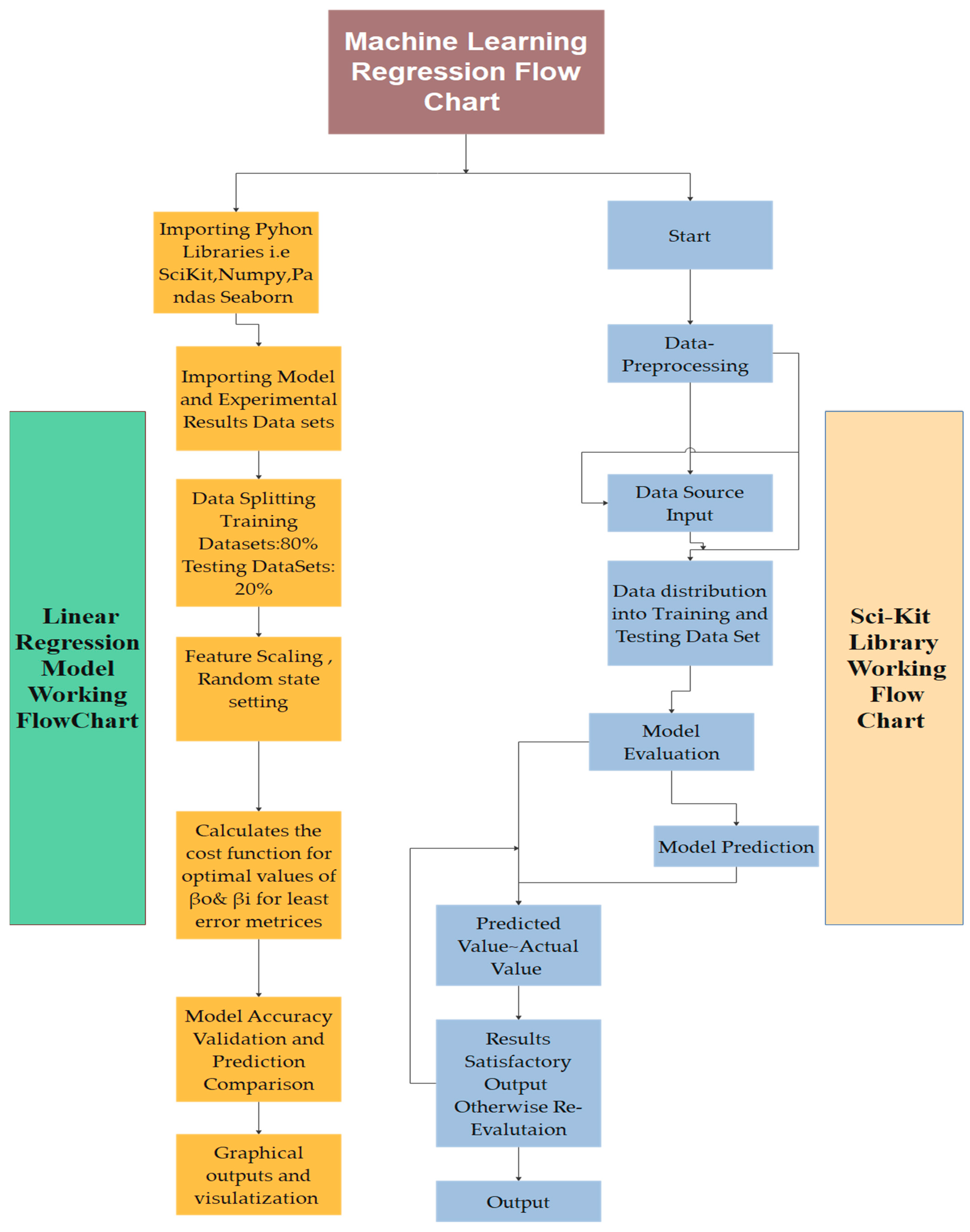
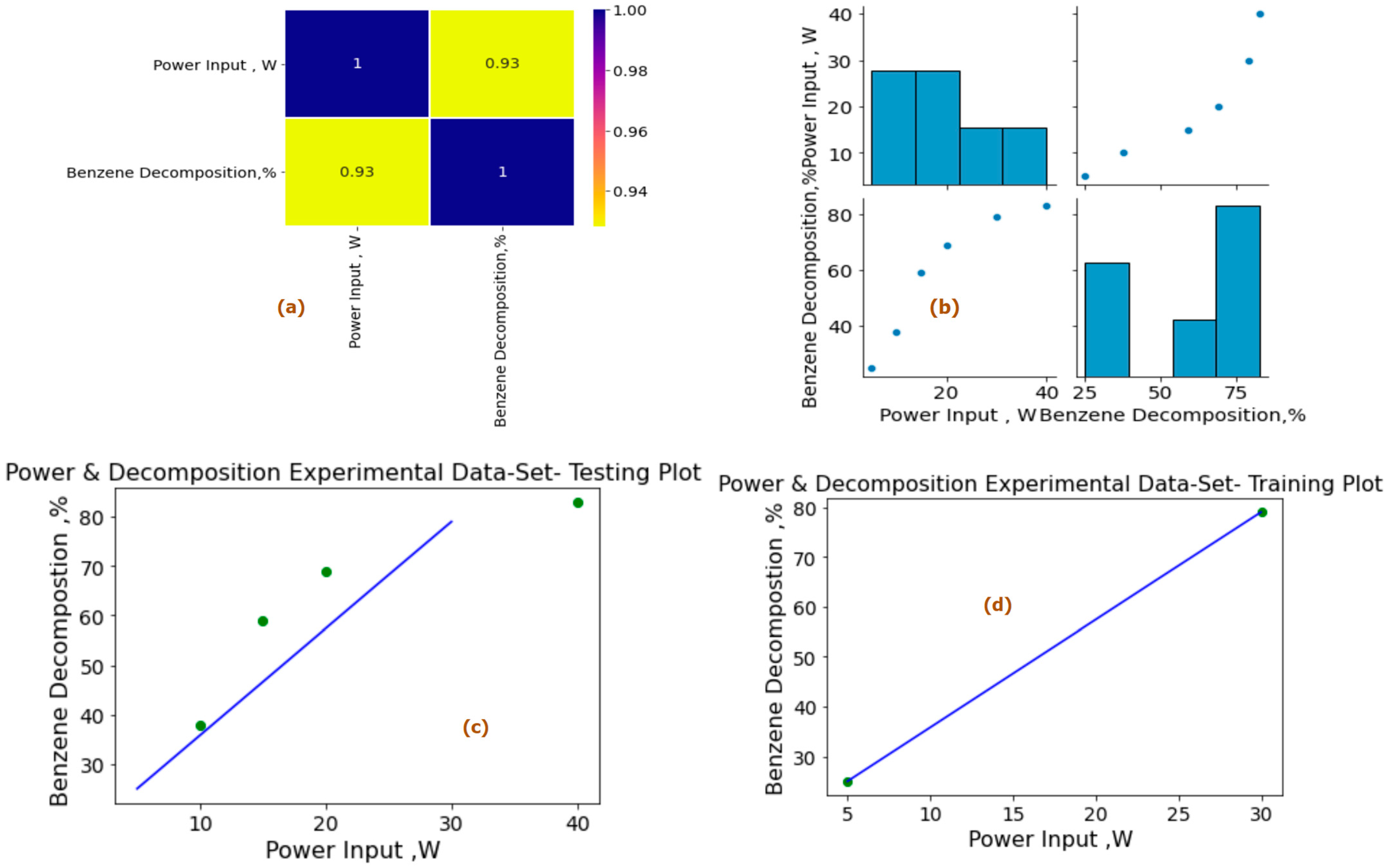
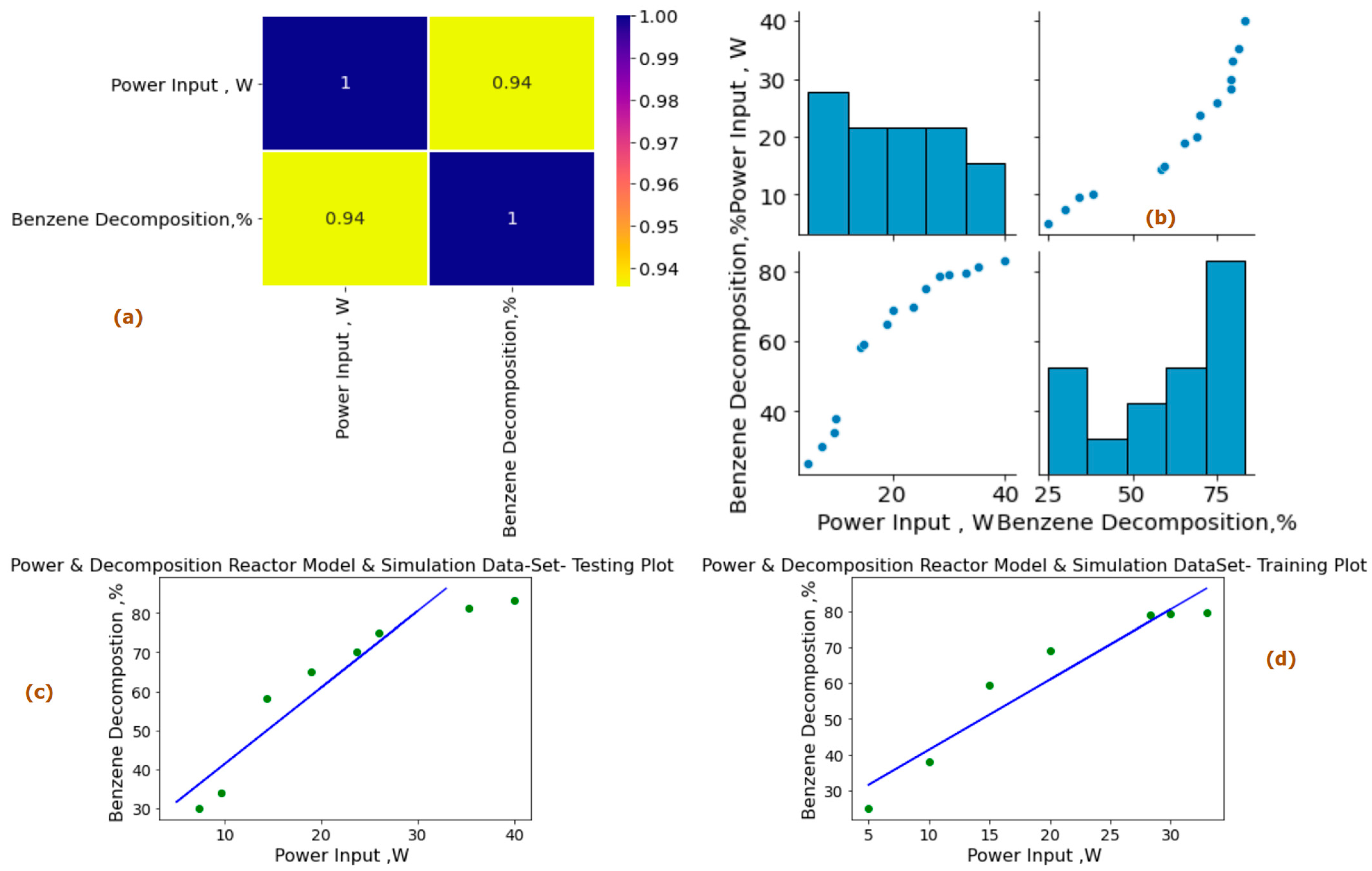
3.3. Machine Learning Algorithms and Predictive Model

Machine learning modules incorporate analyzing and reducing error iteratively by improving and building a better relationship between labels and their corresponding features. In experimentation and modeling research, multiple types of erroneous results are produced. In experimentation, the nature of results varies from a few points to a bulk of datasets. Raw data are classified and categorized according to research outcomes. In plasma engineering, thermal and non-thermal plasma kinetics are in two distinct sets i.e., equilibrium and non-equilibrium. Great work has been done in thermal plasma engineering for validating CFD results, EEFDF datasets, kinetics, yield forecasting, etc. Due to the advancement in the field of data-driven plasma engineering, mainly due to the electrification of process industries, greater emphasis is needed on machine learning modules for kinetic modeling of NTP reactors and reactions for scale-up and design studies. In NTP kinetics, available datasets have such variables as power inputs (P_in), specific input energy (SIE), reactant conversions (X_a), reactant concentration (C_a), product yield (Y_a), flow rates (Q), removal efficiency, etc. The pattern of influence of variables on each other is classified as linear or nonlinear graphically. In the current study, variables such as inlet tar concentration, plasma power input, and residence time are of prime importance during experimental and current kinetic modeling and reactor model simulation. However, the R² value, as discussed in the experimental section, has significant deviation in terms of power input and analogue compound decomposition, i.e., R² = 0.865, while all other variables studies have an R² value of 0.99.

3.4. Mathematical Understanding Machine Learning Linear Regression Algorithm

Regression algorithms are divided into linear algorithms and nonlinear algorithms for bivariate and multivariate conditions by using linear and polynomial regression algorithms [55]. Regression algorithms are classically incorporated using ordinary least square regression methods, stepwise linear regression, linear regression, local estimate scatterplot smoothing, and stepwise regression [56]. Classification of regression for open and closed-form solutions is found in [57,58].

The basics of LR, MLR, MLPR are:

$$Y=mx+b$$

(23)

where Y is the independent variable, X is the independent variable, m is the slope of the line and C is the intercept, as shown in Figure 8. This is the simplest linear regression usually incorporated into kinetic modeling. The simplest LR model produces the best-fit line that passes closest to the maximum likelihood point with a minimum error or Euclidian distance [59]. LR is based on either a closed-form solution or a non-closed solution for slope and intercepts calculations without calculus derivatives and integration. Modified linear regression machine learning is a popular model with a simplified assumption of linear entanglement between the system input variable and corresponding output variable results [60]. The dataset is uniquely continuously numeric. In LR, a y target value is assumed to be dependent on the X (x₁, …, x_n) and residual random error. For an n^th generalized observation model dataset, the modified relationship is as follows:

$$y={\beta }_o+{\beta }_1{x}_{n1}+{\beta }_2{x}_{n2}+\cdots +{\beta }_d{x}_{nd}+{\epsilon }_n$$

(24)

The intercept terms ${\beta }_o$ and ${\beta }_1$ to ${\beta }_D$ are the feature variable coefficients with a randomized error ${\epsilon }_{}$. Error is the difference between the true value (y) and the predicted value (Y_i) [38,39], as shown in Figure 8. The LR algorithm gives an estimation of β coefficient-related parameters. Estimated parameters ${{\beta }^e}_0,\dots , {{\beta }^e}_D$ give an estimated target value of the variable ${{ y}^e}_n$. The LR algorithm gives the best values for βo and β₁, with minimum error residual ε indicating the synergy between predicted y_pred and actual values y_i of experimentation and machine learning model prediction. Different parameters are involved in the error reduction and regression method for synchronizing the results and producing an R² value closer to 1 [47,48].

$${\epsilon }_n=y_{predict }-y_i$$

(25)

$$\therefore y_{predict }={\beta }_o+{\beta }_i{x}_i$$

(26)

Best-fit lines cross through a maximum point of scatter plot. The line is obtained through the minimization of the residual sum of squares (RSS) and mean square error (MSE). A cost function is a minimum for RSS and MSE values. The LR algorithm gives the cost function for optimal values of ${\beta }_o\& {\beta }_i$ for the best-fitting vector positioning [61].

3.5. Model Evaluation Metrics

In order to enhance the accuracy of the ML prediction system, the ML linear regression (LR) model is evaluated using a set of key metrics. Favorable conditions for ML running the LR model include low variance and higher bias, as they contribute to improved prediction accuracy and faster computation, albeit with a greater number of assumptions [61,62]. One important metric used is the R² or determination of R² coefficient. This metric calculates the variance in the developed model for ML prediction results and ranges between 0 and 1. A higher R² indicates greater applicability and better prediction results of the model. Another metric employed is the root mean square error (RMSE). This metric measures the residual variance, taking the square root of the difference between the observed data and predicted values. RMSE considers the degree of freedom for unbiasedness estimation and corresponds to the residual standard error (RSE).

$$R^2=1-\left(\frac{(\sum _{i=1}^n\left(y_i-{\beta }_o-{\beta }_i{)}^2\right)}{(y_i-\overline{y}{)}^2}\right)$$

(27)

$$RMSE=\sqrt{\left(\frac{(\sum _{i=1}^n\left(y_{i^{actual}}-y_{i^{pred}}{)}^2\right)}{\left(n\right)}\right)}$$

(28)

$$RSE=\sqrt{\left(\frac{(\sum _{i=1}^n\left(y_{i^{actual}}-y_{i^{pred}}{)}^2\right)}{\left(n-2\right)}\right)}$$

(29)

The analysis of the experimental data in this study reveals important insights into the relationship between various variables. The power input in NTP reactors is of significant interest, as it is less likely to be temperature-dependent. Moreover, the kinetic modeling techniques employed, such as power-law kinetics, heavily rely on the input power (Figure 9). Therefore, the power input energy variable has been shortlisted as a key factor for the machine learning-based black box modeling.

To further explore these relationships, heat maps were generated using Python built-in libraries. These heat maps visually depict the interdependence among the variables, with Figure 10a and Figure 11a showcasing the relationships between power input (P_in, W), and tar analogue decomposition (X_a, %), while Figure 10b and Figure 11b focus on the shortlisted variables under experimental conditions—power input (pin, W) and experimental decomposition (X_A within the range of 0–100%)—for preprocessing of available experimental and reactor model and simulation datasets. The heat maps and paired plots provide valuable insights into the linearity and correlation between these variables, with inlet compound decomposition (%) and power input exhibiting significant correlation coefficients of 0.93 and 0.94, respectively, from the experimental and reactor model simulations. The subsequent analysis of linearly dependent variable data presented also shows our proposed metrics showed a higher dependence of variables in the modeling and simulation dataset in comparison to the experimental dataset, as well as relatively less noise in data and effective overall trend for scale-up studies.

In our case studies, the input power in the experimental and reactor model is similar in pattern with performance metrics of R² of 0.865 and 0.889, as shown in Figure 10 and Figure 11. In comparison to the absolute effective value of defining the global approach of model results to be incorporated in the current studies, in the graphs shown below, raw data of experimental conditions and reactor models are plotted. Raw data are further classified for feature engineering, data distribution, standard deviation, loss function reduction, cost function penalization, and metrics-based performance assessment to increase the model validation by tuning the slope or intercept through learning rate for model accuracy, mean square error (MSE), root mean square error (RMSE), sum of the square of error (SSE), R², and adjusted R². In ML modules, the error function is iterated for the minimum results. Each loop of commands produces a significant difference in error, and related features are optimized for the best results output. In ML regression conditions, the raw dataset is calculated from the source. Figure 9 shows that the two datasets are optimally available. The total dataset consists of 60 sample values. Design-Expert software was used for increasing the number of experimentation dataset sample values at similar trends using a built-in function.

The input dataset is first quantitatively aligned and according to outliers and central distribution tendency results are produced using the preprocessing statistical functions in Python programming. Spyder Compiler is used for computation and algorithmic studies. A complete overview of Python libraries and a general machine learning linear algorithm flowchart are shown in Figure 9. The dataset is divided into 45% training sets and 55% testing sets, as illustrated in Figure 10c,d and Figure 11c,d for the experimental and modeling datasets, respectively. A higher percentage of the testing dataset is utilized due to the limited number of values available in the experimental data. This approach allows for an extended analysis and provides a comprehensive understanding using a larger portion of the dataset. Consequently, it enables the development of an accurate machine learning model through the training dataset.

The training set reduces the cost function for finding the optimal values of line equation coefficients. Actual values are considered the target values. For each iteration in the machine learning algorithm, a new value for each coefficient for the variable is assigned according to the number of variables. For power input (P_in) vs. reactant decomposition (X), scatter datasets reduce the Euclidean distances for the actual and target results. X_m and X_exp are reduced to a minimum according to the machine learning features and implications. Repeated iteration using the Scikit Learn Library produces a dataset that is validated against the test datasets (approx. 50%) of original datasets for more error reduction in a loop structure. The machine learning model is deployed for new datasets after successful completion. ML prediction values are designated for mean square error (MSE), root mean square error (RMSE), sum of the square of error (SSE), R², and adjusted R² for model accuracy.

ML-LR revolves around the comprehensive analysis of the results obtained from the experiment, reactor model simulations, and machine learning predictions, as presented in

Table 1. Machine learning linear regression model evaluation of experimental and reactor modeling and simulation dataset.

Metrics	ML-Experiment Results	ML-Reactor Model and Simulations	Overall- Machine Learning Predictions
Intercept	2.16	1.95795433	1.91
Linear Coefficient	14.2	21.74562448	23.1
Training Set	45%	45%	45%
Testing Sets	55%	55%	55%
R2 Value	0.86	0.88	0.998
Mean Absolute Error (MAE)	0.0978	0.032	0.008
Mean Squared Error (MSE)	0.0024	0.001	0.00001
Root Mean Square Error (RMSE)	0.042	0.034	0.019
Adjusted R2	0.865	0.8891	0.9984
Accuracy of Model	0.923545907	0.98876584	0.99918729

, based on the machine learning modeling results of experimental and reactor model and simulation, shown in Figure 10 and Figure 11. The various metrics measured in this study provide valuable insights into the performance and accuracy of the models employed. The intercept values yielded a value of 2.16, indicating a baseline reference point. The reactor model and simulations achieved a slightly lower intercept of 1.95795433, while the machine learning predictions resulted in an intercept of 1.91. These values suggest that both the reactor model and machine learning approach were able to effectively capture the baseline behavior, indicating the accuracy of the models. The linear coefficient was 14.2, which increased to 21.74562448 in the reactor model and simulations. This demonstrates that the reactor model and simulations exhibit a stronger linear relationship between the variables under consideration. Remarkably, the machine learning predictions surpassed both, with a linear coefficient of 23.1, indicating a more pronounced effect of the predictors on the response variable.

In order to evaluate the performance of the models, the dataset division into training and testing sets, with a balanced split for training and testing, ensured that ML-LR results for both the reactor model and simulations and machine learning predictions were evaluated using the same proportion of data as the experiment and also enabled a fair comparison of their capabilities in capturing the underlying patterns and predicting the target variable accurately.

A measure of the goodness of fit, R² provides insights into the proportion of variance explained by the model. The experiment achieved an R² of 0.86, indicating that 86% of the variation in the response variable can be attributed to the predictors considered in the experiment. The reactor model and simulations improved this value to 0.88, showcasing a stronger relationship between the predictors and the response variable. However, the machine learning predictions demonstrated a remarkable R² of 0.998, indicating an exceptional ability to explain the variance in the target variable. This signifies a high level of accuracy and reliability in predicting the desired outcome.

The accuracy of the models accounts for several error metrics. The mean absolute error (MAE) measures the average magnitude of the errors between predicted and actual values. The experiment yielded a MAE of 0.0978, while the reactor model and simulations reduced this error to 0.032. Notably, the machine learning predictions achieved an impressively low MAE of 0.008, indicating superior accuracy and precision. The mean squared error (MSE), which quantifies the average squared differences between predicted and actual values, revealed similar trends. The experiment resulted in an MSE of 0.0024, reduced to 0.001 in the reactor model and simulations. Surprisingly, the machine learning predictions achieved the lowest MSE of 0.00001, further highlighting their ability to minimize errors and provide highly accurate predictions.

The root mean square error (RMSE), an estimation of the standard deviation of the errors, followed a similar pattern. The experiment yielded an RMSE of 0.042, while the reactor model and simulations achieved a lower RMSE of 0.034. Notably, the machine learning predictions achieved the lowest RMSE of 0.019, indicating superior precision and accuracy in predicting the desired outcome. Additionally, the adjusted R², which considers the number of predictors and sample size, followed a similar trend. The experiment obtained an adjusted R² of 0.865, while the reactor model and simulations demonstrated an improved value of 0.8891. Remarkably, the machine learning predictions excelled with an exceptional adjusted R² of 0.9984, emphasizing their ability to accurately account for the variations in the response variable.

The accuracy of the model, indicating the percentage of correct predictions, was evaluated. The experiment achieved an accuracy of 0.923545907, which improved to 0.98876584 in the reactor model and simulations. Remarkably, the machine learning predictions exhibited a significantly higher accuracy of 0.99918729, highlighting their ability to give precise and reliable predictions as well as validation using OLS regression. We are deployed the closed-form solution in Python for the linear regression model. The ordinary least square method is occasionally used for the cross-validation of machine learning models. In comparison to the Scikit Learn Library, the OLS results are less appropriate and accurate due to lesser iteration and drawback of performance in low-bias and high-variance regions with utmost validation. The method, however, gives a good idea about different effective statistical methods, such as Durbin–Watson, Df, F-statistic, and residuals, as shown in

Table 2. Ordinary least square linear regression model evaluation metrics results.

OLS Regression Results
Dependent Variable:	Y		R-squared:		0.890
Model:	OLS		Adj. R-squared:		0.887
Method	Least Squares		F-statistic:		347.9
Number of Observation	60		Prob (F-statistic):		3.14 × 10−22
Df Residuals	43		Log-likelihood		75.111
Df Model:	1		AIC		−146.2
Covariance Type:	robust		BIC		−142.6
Omnibus:	4.279		Durbin–Watson		0.028
Prob (Omnibus):	0.118		Jarque–Bera (JB):		3.665
Skew:	−0.63		Prob (JB)		0.160
Kurtosis:	2.293		Cond. No		37.5
	Coif	Standard error	T	p > |t|	p < 2.5%	p < 97.5%
Const	0.4420	0.022	20.27	0.00	0.398	0.486
×1	0.0342	0.002	18.64	0.00	0.031	0.038

. Training of datasets from experimentation and reactor model gives a good fit of minimized cost function results in the testing stage with closer collinearity in comparative results. p-values deduced from OLS fitting results had a 0.031 value against the standard 0.05 value for hypothesis testing results, as shown in Table 2. Standard error in the OLS method assumes a covariance matrix for the specific identification of statistical results. In future studies for similar gaseous mixtures, empirical results of machine learning based LR outputs are validated and decomposition percentage for the input power variable at any given similar concentration of the tar analogue compound.

Overall, the results indicate that both the reactor model and simulations and the machine learning predictions outperformed the experiment in various respects. The reactor model and simulations showcased a stronger linear relationship and achieved higher accuracy than the experiment. The machine learning predictions excelled in capturing complex patterns, resulting in exceptional accuracy and precision. These findings emphasize the effectiveness of both modeling approaches, particularly the machine learning technique, in accurately predicting the desired outcomes.

4. Conclusions

Tar is a barrier to full renewable energy exploitation through variable feedstock. NTP technologies define new pathways for tar analogue compound decomposition, removal, and reduction studies with an electrified process. A holistic approach to decomposition uses a study dataset of benzene as a tar analogue compound in a tetra carrier gaseous mixture. Power input, the flow rate of carrier gases, tar analogue compound inlet concentration and residence time against decomposition percentage are considered the input variables for studies in the DBD reactor. An apparent rate constant of 0.040 kJ/L has been calculated at an initial concentration of 36 g/Nm³ of the analogue compound for the power input of 40 W for residence time of 2.86 s. A reactor model for DBD reactor performance assessment and cross-validation of apparent rate decomposition constant has been proposed using definite assumptions. An ODE equation set has been produced by mathematical modeling. Reactor scale length shows similar behavior to the plug flow reactor for the changing conversion. A hotspot region in the initial 15% to 25% of the reactor length is the maximum decomposition patch for the tar analogue compound into associated lighter hydrocarbons and soot. Furthermore, the model run for the pin ranges from 5 W to 40 W, and a constant flow rate of 40 mL/min of carrier flow gas mixture of methane and nitrogen shows considerable synergetic results, with a maximum decomposition of 83.01% against 82.9% experimentation decomposition. However, statistical data analysis of experimental and reactor model datasets shows the difference in metrics value i.e., R². A new and advanced Python programming machine learning tool has been used for error reduction in experimentation and reactor model results for generalized empirical formulation in scale-up studies. ML linear regression algorithm takes into account the experimental and reactor datasets. Datasets are divided into training and testing datasets. This reduces the RME, MSE, MAE, and R² errors for the datasets and produces a prediction model for new intercepts and slopes with minimum cost functions: ML R²~1 for the experimental and reactor model datasets against original R² = 0.85 and 0.89 value.

References

1. Yousaf, A.M.; Aqsa, R. Integrating Circular Economy, SBTI, Digital LCA, and ESG Benchmarks for Sustainable Textile Dyeing: A Critical Review of Industrial Textile Practices. Glob. NEST J. 2023. [Google Scholar] [CrossRef]
2. Ryšavý, J.; Serenčíšová, J.; Horák, J.; Ochodek, T. The Co-Combustion of Pellets with Pistachio Shells in Residential Units Additionally Equipped by Pt-Based Catalyst. Biomass Convers. Biorefin. 2023, 1–17. [Google Scholar] [CrossRef]
3. Abdelaziz, A.A.; Ishijima, T.; Seto, T. Humidity Effects on Surface Dielectric Barrier Discharge for Gaseous Naphthalene Decomposition. Phys. Plasmas 2018, 25, 043512. [Google Scholar] [CrossRef]
4. Abdelaziz, A.A.; Seto, T.; Abdel-Salam, M.; Otani, Y. Performance of a Surface Dielectric Barrier Discharge Based Reactor for Destruction of Naphthalene in an Air Stream. J. Phys. D Appl. Phys. 2012, 45, 115201. [Google Scholar] [CrossRef] [Green Version]
5. Affonso Nóbrega, P.H.; Rohani, V.; Fulcheri, L. Non-Thermal Plasma Treatment of Volatile Organic Compounds: A Predictive Model Based on Experimental Data Analysis. Chem. Eng. J. 2019, 364, 37–44. [Google Scholar] [CrossRef]
6. Affonso Nobrega, P.; Gaunand, A.; Rohani, V.; Cauneau, F.; Fulcheri, L. Applying Chemical Engineering Concepts to Non-Thermal Plasma Reactors. Plasma Sci. Technol. 2018, 20, 065512. [Google Scholar] [CrossRef] [Green Version]
7. Sieradzka, M.; Mlonka-Mędrala, A.; Kalemba-Rec, I.; Reinmöller, M.; Küster, F.; Kalawa, W.; Magdziarz, A. Evaluation of Physical and Chemical Properties of Residue from Gasification of Biomass Wastes. Energies 2022, 15, 3539. [Google Scholar] [CrossRef]
8. Ziółkowski, P.; Madejski, P.; Amiri, M.; Kuś, T.; Stasiak, K.; Subramanian, N.; Pawlak-Kruczek, H.; Badur, J.; Niedźwiecki, Ł.; Mikielewicz, D. Thermodynamic Analysis of Negative CO2 Emission Power Plant Using Aspen Plus, Aspen Hysys, and Ebsilon Software. Energies 2021, 14, 6304. [Google Scholar] [CrossRef]
9. Čespiva, J.; Skřínský, J.; Vereš, J.; Borovec, K.; Wnukowski, M. Solid-Recovered Fuel to Liquid Conversion Using Fixed Bed Gasification Technology and a Fischer–Tropsch Synthesis Unit–Case Study. Int. J. Energy Prod. Manag. 2020, 5, 212–222. [Google Scholar] [CrossRef]
10. Skřínský, J.; Vereš, J.; Čespiva, J.; Ochodek, T.; Borovec, K.; Koloničný, J. Explosion Characteristics of Syngas from Gasification Process. J. Pol. Miner. Eng. Soc. 2020, January-Ju, 195–200. [Google Scholar] [CrossRef]
11. Carotenuto, A.; Di Fraia, S.; Massarotti, N.; Sobek, S.; Uddin, M.R.; Vanoli, L.; Werle, S. Predictive Modeling for Energy Recovery from Sewage Sludge Gasification. Energy 2023, 263, 125838. [Google Scholar] [CrossRef]
12. Vishwajeet; Pawlak-Kruczek, H.; Baranowski, M.; Czerep, M.; Chorążyczewski, A.; Krochmalny, K.; Ostrycharczyk, M.; Ziółkowski, P.; Madejski, P.; Mączka, T.; et al. Entrained Flow Plasma Gasification of Sewage Sludge–Proof-of-Concept and Fate of Inorganics. Energies 2022, 15, 1948. [Google Scholar] [CrossRef]
13. Werle, S.; Dudziak, M. Analysis of Organic and Inorganic Contaminants in Dried Sewage Sludge and By-Products of Dried Sewage Sludge Gasification. Energies 2014, 7, 462–476. [Google Scholar] [CrossRef] [Green Version]
14. Čespiva, J.; Niedzwiecki, L.; Wnukowski, M.; Krochmalny, K.; Mularski, J.; Ochodek, T.; Pawlak-Kruczek, H. Torrefaction and Gasification of Biomass for Polygeneration: Production of Biochar and Producer Gas at Low Load Conditions. Energy Rep. 2022, 8, 134–144. [Google Scholar] [CrossRef]
15. Čespiva, J.; Wnukowski, M.; Niedzwiecki, L.; Skřínský, J.; Vereš, J.; Ochodek, T.; Pawlak-Kruczek, H.; Borovec, K. Characterization of Tars from a Novel, Pilot Scale, Biomass Gasifier Working under Low Equivalence Ratio Regime. Renew. Energy 2020, 159, 775–785. [Google Scholar] [CrossRef]
16. Peck, D.; Zappi, M.; Gang, D.; Guillory, J.; Hernandez, R.; Buchireddy, P. Review of Porous Ceramics for Hot Gas Cleanup of Biomass Syngas Using Catalytic Ceramic Filters to Produce Green Hydrogen/Fuels/Chemicals. Energies 2023, 16, 2334. [Google Scholar] [CrossRef]
17. Anis, S.; Zainal, Z.A. Tar Reduction in Biomass Producer Gas via Mechanical, Catalytic and Thermal Methods: A Review. Renew. Sustain. Energy Rev. 2011, 15, 2355–2377. [Google Scholar] [CrossRef]
18. Font Palma, C. Modelling of Tar Formation and Evolution for Biomass Gasification: A Review. Appl. Energy 2013, 111, 129–141. [Google Scholar] [CrossRef]
19. Papa, A.A.; Savuto, E.; Di Carlo, A.; Tacconi, A.; Rapagnà, S. Synergic Effects of Bed Materials and Catalytic Filter Candle for the Conversion of Tar during Biomass Steam Gasification. Energies 2023, 16, 595. [Google Scholar] [CrossRef]
20. Kochel, M.; Szul, M.; Iluk, T.; Najser, J. On the Possibility of Cleaning Producer Gas Laden with Large Quantities of Tars through Using a Simple Fixed-Bed Activated Carbon Adsorption Process. Energies 2022, 15, 7433. [Google Scholar] [CrossRef]
21. Yang, C.; Ying, K.; Yang, F.; Peng, H.; Chen, Z. Simulation on the Electric and Thermal Fields of a Microwave Reactor for Ex Situ Biomass Tar Elimination. Energies 2022, 15, 4143. [Google Scholar] [CrossRef]
22. Wnukowski, M.; Kordylewski, W.; Łuszkiewicz, D.; Leśniewicz, A.; Ociepa, M.; Michalski, J. Sewage Sludge-Derived Producer Gas Valorization with the Use of Atmospheric Microwave Plasma. Waste Biomass Valorization 2020, 11, 4289–4303. [Google Scholar] [CrossRef] [Green Version]
23. Wnukowski, M.; Moroń, W. Warm Plasma Application in Tar Conversion and Syngas Valorization: The Fate of Hydrogen Sulfide. Energies 2021, 14, 7383. [Google Scholar] [CrossRef]
24. Dors, M.; Kurzyńska, D. Tar Removal by Nanosecond Pulsed Dielectric Barrier Discharge. Appl. Sci. 2020, 10, 991. [Google Scholar] [CrossRef] [Green Version]
25. Valderrama Rios, M.L.; González, A.M.; Lora, E.E.S.; Almazán del Olmo, O.A. Reduction of Tar Generated during Biomass Gasification: A Review. Biomass Bioenergy 2018, 108, 345–370. [Google Scholar] [CrossRef]
26. Fourcault, A.; Marias, F.; Michon, U. Modelling of Thermal Removal of Tars in a High Temperature Stage Fed by a Plasma Torch. Biomass Bioenergy 2010, 34, 1363–1374. [Google Scholar] [CrossRef]
27. Fuentes-Cano, D.; Gómez-Barea, A.; Nilsson, S.; Ollero, P. Decomposition Kinetics of Model Tar Compounds over Chars with Different Internal Structure to Model Hot Tar Removal in Biomass Gasification. Chem. Eng. J. 2013, 228, 1223–1233. [Google Scholar] [CrossRef]
28. Gadkari, S.; Gu, S. Numerical Investigation of Co-Axial DBD: Influence of Relative Permittivity of the Dielectric Barrier, Applied Voltage Amplitude, and Frequency. Phys. Plasmas 2017, 24, 053517. [Google Scholar] [CrossRef]
29. Harling, A.M.; Glover, D.J.; Whitehead, J.C.; Zhang, K. Novel Method for Enhancing the Destruction of Environmental Pollutants by the Combination of Multiple Plasma Discharges. Environ. Sci. Technol. 2008, 42, 4546–4550. [Google Scholar] [CrossRef]
30. Jiang, N.; Lu, N.; Li, J.; Wu, Y. Degradation of Benzene by Using a Silent-Packed Bed Hybrid Discharge Plasma Reactor. Plasma Sci. Technol. 2012, 14, 140–146. [Google Scholar] [CrossRef]
31. Karatum, O.; Deshusses, M.A. A Comparative Study of Dilute VOCs Treatment in a Non-Thermal Plasma Reactor. Chem. Eng. J. 2016, 294, 308–315. [Google Scholar] [CrossRef]
32. Kong, X.; Zhang, H.; Li, X.; Xu, R.; Mubeen, I.; Li, L.; Yan, J. Destruction of Toluene, Naphthalene and Phenanthrene as Model Tar Compounds in a Modified Rotating Gliding Arc Discharge Reactor. Catalysts 2018, 9, 19. [Google Scholar] [CrossRef] [Green Version]
33. Saleem, F.; Khoja, A.H.; Umer, J.; Ahmad, F.; Abbas, S.Z.; Zhang, K.; Harvey, A. Removal of Benzene as a Tar Model Compound from a Gas Mixture Using Non-Thermal Plasma Dielectric Barrier Discharge Reactor. J. Energy Inst. 2021, 96, 97–105. [Google Scholar] [CrossRef]
34. Huang, Z.; Wang, Y.; Dong, N.; Song, D.; Lin, Y.; Deng, L.; Huang, H. In Situ Removal of Benzene as a Biomass Tar Model Compound Employing Hematite Oxygen Carrier. Catalysts 2022, 12, 1088. [Google Scholar] [CrossRef]
35. Park, H.J.; Park, S.H.; Sohn, J.M.; Park, J.; Jeon, J.-K.; Kim, S.-S.; Park, Y.-K. Steam Reforming of Biomass Gasification Tar Using Benzene as a Model Compound over Various Ni Supported Metal Oxide Catalysts. Bioresour. Technol. 2010, 101, S101–S103. [Google Scholar] [CrossRef]
36. Saleem, F.; Abbas, A.; Rehman, A.; Khoja, A.H.; Naqvi, S.R.; Arshad, M.Y.; Zhang, K.; Harvey, A. Decomposition of Benzene as a Biomass Gasification Tar in CH4 Carrier Gas Using Non-Thermal Plasma: Parametric and Kinetic Study. J. Energy Inst. 2022, 102, 190–195. [Google Scholar] [CrossRef]
37. Liang, W.; Sun, H.; Shi, X.; Zhu, Y. Abatement of Toluene by Reverse-Flow Nonthermal Plasma Reactor Coupled with Catalyst. Catalysts 2020, 10, 511. [Google Scholar] [CrossRef]
38. Saleem, F.; Umer, J.; Rehman, A.; Zhang, K.; Harvey, A. Effect of Methane as an Additive in the Product Gas toward the Formation of Lower Hydrocarbons during the Decomposition of a Tar Analogue. Energy Fuels 2020, 34, 1744–1749. [Google Scholar] [CrossRef]
39. Saleem, F.; Zhang, K.; Harvey, A. Role of CO2 in the Conversion of Toluene as a Tar Surrogate in a Nonthermal Plasma Dielectric Barrier Discharge Reactor. Energy Fuels 2018, 32, 5164–5170. [Google Scholar] [CrossRef] [Green Version]
40. Tay, W.H.; Kausik, S.S.; Wong, C.S.; Yap, S.L.; Muniandy, S.V. Statistical Modelling of Discharge Behavior of Atmospheric Pressure Dielectric Barrier Discharge. Phys. Plasmas 2014, 21, 113502. [Google Scholar] [CrossRef]
41. Liu, S.Y.; Mei, D.H.; Shen, Z.; Tu, X. Nonoxidative Conversion of Methane in a Dielectric Barrier Discharge Reactor: Prediction of Reaction Performance Based on Neural Network Model. J. Phys. Chem. C 2014, 118, 10686–10693. [Google Scholar] [CrossRef]
42. Wang, D.; Yuan, W.; Ji, W. Char and Char-Supported Nickel Catalysts for Secondary Syngas Cleanup and Conditioning. Appl. Energy 2011, 88, 1656–1663. [Google Scholar] [CrossRef]
43. Wang, T.C.; Lu, N.; Li, J.; Wu, Y. Degradation of Pentachlorophenol in Soil by Pulsed Corona Discharge Plasma. J. Hazard. Mater. 2010, 180, 436–441. [Google Scholar] [CrossRef]
44. Jamróz, P.; Kordylewski, W.; Wnukowski, M. Microwave Plasma Application in Decomposition and Steam Reforming of Model Tar Compounds. Fuel Process. Technol. 2018, 169, 1–14. [Google Scholar] [CrossRef]
45. Saleem, F.; Harris, J.; Zhang, K.; Harvey, A. Non-Thermal Plasma as a Promising Route for the Removal of Tar from the Product Gas of Biomass Gasification–A Critical Review. Chem. Eng. J. 2020, 382, 122761. [Google Scholar] [CrossRef]
46. Saleem, F.; Harvey, A.; Zhang, K. Low Temperature Conversion of Toluene to Methane Using Dielectric Barrier Discharge Reactor. Fuel 2019, 248, 258–261. [Google Scholar] [CrossRef]
47. Saleem, F.; Zhang, K.; Harvey, A. Plasma-Assisted Decomposition of a Biomass Gasification Tar Analogue into Lower Hydrocarbons in a Synthetic Product Gas Using a Dielectric Barrier Discharge Reactor. Fuel 2019, 235, 1412–1419. [Google Scholar] [CrossRef] [Green Version]
48. Saleem, F.; Zhang, K.; Harvey, A. Temperature Dependence of Non-Thermal Plasma Assisted Hydrocracking of Toluene to Lower Hydrocarbons in a Dielectric Barrier Discharge Reactor. Chem. Eng. J. 2019, 356, 1062–1069. [Google Scholar] [CrossRef] [Green Version]
49. Pineau, A.; Chimier, B.; Hu, S.X.; Duchateau, G. Modeling the Electron Collision Frequency during Solid-to-Plasma Transition of Polystyrene Ablator for Direct-Drive Inertial Confinement Fusion Applications. Phys. Plasmas 2020, 27, 092703. [Google Scholar] [CrossRef]
50. Ratkiewicz, A.; Truong, T.N. A Canonical Form of the Complex Reaction Mechanism. Energy 2012, 43, 64–72. [Google Scholar] [CrossRef]
51. Robicheaux, F.; Hanson, J.D. Simulated Expansion of an Ultra-Cold, Neutral Plasma. Phys. Plasmas 2003, 10, 2217–2229. [Google Scholar] [CrossRef]
52. Rostami, R.; Moussavi, G.; Jafari, A.J.; Darbari, S. Abatement of Benzene in Sequential NTP -Influence of Operational Factors. Int. J. Plasma Environ. Sci. Technol. 2019, 13, 26–31. [Google Scholar] [CrossRef]
53. Filimonova, E.A.; Naidis, G. V Effect of Gas Mixture Composition on Tar Removal Process in a Pulsed Corona Discharge Reactor. J. Phys. Conf. Ser. 2010, 257, 012018. [Google Scholar] [CrossRef]
54. Filimonova, E.A.; Amirov, R.H.; Kim, H.T.; Park, I.H. Comparative Modelling of NO x and SO 2 Removal from Pollutant Gases Using Pulsed-Corona and Silent Discharges. J. Phys. D Appl. Phys. 2000, 33, 1716–1727. [Google Scholar] [CrossRef]
55. Ma, P. A New Partially-Coupled Recursive Least Squares Algorithm for Multivariate Equation-Error Systems. Int. J. Control Autom. Syst. 2023, 21, 1828–1839. [Google Scholar] [CrossRef]
56. Voigt, T.; Kohlhase, M.; Nelles, O. Incremental DoE and Modeling Methodology with Gaussian Process Regression: An Industrially Applicable Approach to Incorporate Expert Knowledge. Mathematics 2021, 9, 2479. [Google Scholar] [CrossRef]
57. Yar, A.; Arshad, M.Y.; Asghar, F.; Amjad, W.; Asghar, F.; Hussain, M.I.; Lee, G.H.; Mahmood, F. Machine Learning-Based Relative Performance Analysis of Monocrystalline and Polycrystalline Grid-Tied PV Systems. Int. J. Photoenergy 2022, 2022, 3186378. [Google Scholar] [CrossRef]
58. Yousaf, M.A.; Rashid, A.; Gul, H.; Ahmad, A.S.; Jabbar, F. Optimization of Acid-Assisted Extraction of Pectin from Banana (Musa Acuminata) Peels by Central Composite Design. Glob. NEST J. 2022, 24, 752–756. [Google Scholar] [CrossRef]
59. Cebekhulu, E.; Onumanyi, A.J.; Isaac, S.J. Performance Analysis of Machine Learning Algorithms for Energy Demand–Supply Prediction in Smart Grids. Sustainability 2022, 14, 2546. [Google Scholar] [CrossRef]
60. Yang, X.; Guo, X.; Ouyang, H.; Li, D. A Kriging Model Based Finite Element Model Updating Method for Damage Detection. Appl. Sci. 2017, 7, 1039. [Google Scholar] [CrossRef] [Green Version]
61. Gul, H.; Arshad, M.Y.; Tahir, M.W. Production of H2 via Sorption Enhanced Auto-Thermal Reforming for Small Scale Applications-A Process Modeling and Machine Learning Study. Int. J. Hydrogen Energy 2023, 48, 12622–12635. [Google Scholar] [CrossRef]
62. Arshad, M.Y.; Rashid, A.; Mahmood, F.; Saeed, S.; Ahmed, A.S. Metal(II) Triazole Complexes: Synthesis, Biological Evaluation, and Analytical Characterization Using Machine Learning-Based Validation. Eur. J. Chem. 2023, 14, 155–164. [Google Scholar] [CrossRef]
Figure 2. Working cycle for current TAC decomposition in NTP DBD reactor for kinetic modeling, reactor simulation and machine learning modeling.
Energies 16 05835 g002
Figure 3. Experimental trends for tar analogue compound benzene reduction in DBD reactor (adapted from [36]). (a) Power input (W) vs. benzene decomposition (%) and methane decomposition (%). Pin = 5–40 W, Tin = ambient conditions, Qin = 40 mL/min, concentration = 36 g/Nm3 and t = 2.86 s. (b) Residence time (s) vs. benzene decomposition (%). Tin = ambient conditions, pin = 20 W, concentration = 36 g/Nm3 and t = 0.8–2.86 s. (c) Benzene concentration (g/Nm3) vs. benzene decomposition (%). Tin = ambient conditions, pin = 15 W, concentration = 18, 36, 64 g/Nm3 and t = 2.86 s.
Energies 16 05835 g003
Figure 4. Novel suggested strategy for kinetic modeling, reactor assessment and machine learning methodology.
Energies 16 05835 g004
Figure 5. Decomposition rate-constant calculation.
Energies 16 05835 g005
Figure 6. MATLAB simulation results for TAC reactant concentration (CA) change along the reactor length to product (CB) at t = 2.86 s, Pin = 15 W, Simulation 1 for CA = 0.178 kmol/m3. Simulation 2 for CA = 0.401 kmol/m3 in comparison to experiments of Faisal et al. [36] with simulation. Simulation 3 for CA = 0.801 kmol/m3.
Energies 16 05835 g006
Figure 7. MATLAB simulation results for benzene decomposition at t = 2.86 s, Pin = 5–40 W, simulation for CA = 36 g/Nm3 (0.401 kmol/m3) for experimental and reactor model comparisons of experiments of Faisal et al. [36] with simulation.
Energies 16 05835 g007
Figure 8. Linear regression machine learning error quantification graphical representation.
Energies 16 05835 g008
Figure 9. Machine learning linear regression modeling flowchart for Scikit Learn Library and generalized machine learning linear regression algorithm.
Energies 16 05835 g009
Figure 10. Power input (Pin, W) vs. tar analogue compound decomposition experimental dataset machine learning study (%). (a) Heat map for data analysis. (b) Paired plot of data preprocessing. (c) Experimental dataset testing plot. (d) Experimental training set data plot for shortlisted variable at experimental power input (Pin, W). Experimental decomposition 0–100%, residence time = 2.86 s, concentration = 36 g/Nm3.
Energies 16 05835 g010
Figure 11. Power input (Pin, W) vs. tar analogue compound decomposition reactor model—simulation dataset machine learning study (%). (a) Heat map for data analysis. (b) Paired plot of data preprocessing. (c) Experimental dataset testing plot. (d) Experimental training set data plot for shortlisted variable at experimental power input (Pin, W) in reactor model and simulation dataset conditions. Power input Pin 5–40 W, reactor model and simulation dataset decomposition 0–100%, residence time = 2.86 s, concentration = 36 g/Nm3.
Energies 16 05835 g011