1. Introduction
The impact of residential inverter energy systems (IES) on distribution networks throughout the past decade has been an intensely studied and discussed subject for distribution network operators worldwide. The rapid uptake of renewable generation in Australia, specifically rooftop PV, is a result of network feed-in tariffs combined with falling costs of PV systems, driven by an overarching transition in consumer attitude toward a decarbonized, greener energy future [
1].
The state of Queensland (Qld) in Australia has the highest levels of residential rooftop PV penetration by both capacity and percentage of dwellings [
2]. High levels of IES penetration on distribution feeders can lead to a host of power quality, plant rating, and network issues, including voltage rise, voltage unbalance, harmonic emissions, reverse power flow, poor power factor, and exceedance of plant ratings [
3]. As a result, Energy Queensland, the distribution network service provider for Queensland, has been experiencing voltage rise excursions beyond statutory limits, as well as reverse power flows on distribution feeders [
4].
Voltage rise occurs because for solar PV inverters to export power to the network, they must increase the electrical potential to above that of the network. This effect is exacerbated by the aggregation of many solar PV inverters on the same network.
Currently, it is somewhat easy to determine the inverters’ impact on the network since solar PV inverters up until recently had a fixed power factor of 0.9 lagging, as defined by the Australian Standards at the time. However, in Australia, all new inverter installations from 2021 onwards must comply with the volt–var and volt–watt response modes as stated in the Australian Standard AS4777.2.2020 Inverter Requirements Standard [
5]. These modes control the inverters’ active and reactive power output, respectively, depending on the grid voltage. This dynamic response makes it hard to forecast feeder characteristics using standard steady-state load flow calculations, a challenge that this research seeks to overcome using quasi-dynamic analysis techniques.
Research Motivation and Proposed Approach
The aim of this research was to investigate the automation of modeling Energy Queensland’s low-voltage (LV) networks in DIgSILENT PowerFactory and analyze the distribution network effects of forecast levels of solar PV, including active and reactive power levels and voltage rise, the results of which will be used to formulate trend equations that will provide a simplistic method of approximating network characteristics for other feeders under various levels of IES penetration. Achieving this would elevate the requirement for network planning engineers to conduct detailed network modeling and analyses when assessing the future impacts of IES penetration on distribution networks.
In satisfying the research aim, the following objectives must be met:
Automate the process of constructing LV networks in DIgSILENT PowerFactory, onto the already existing medium voltage (MV) network models;
Automate the process of analyzing LV networks in DIgSILENT PowerFactory;
Interpret and present resulting data in a way that is meaningful and usable.
Modeling LV networks and determining forecasts enables the ability to estimate active and reactive power, voltage, and power factor across distribution networks, as well as how much customers will export energy and experience curtailment of solar PV generation [
6].
This is a two-part process:
First, a script was developed to automate the modeling of LV networks onto the LV buses of distribution transformers in Energy Queensland’s existing distribution models (existing models go down as far as the transformer LV terminals; this project looked to expand all the way to the customer premises);
Each distribution feeder was then analyzed using forecast levels of rooftop solar PV installations and minimum underlying load for each year. Again, this process was automated through a Python script. Minimum load forecasts are used to determine the worst-case effects of rooftop solar PV, as this coincides with maximum power being exported to the grid.
2. Background
2.1. Generalised Overview
The network effects of the high IES penetration on distribution feeders is a well-researched topic in the power industry, as distributed generation has rapidly become a fundamental component of the electricity system [
7].
The advent of customer generation has seen a reverse of the traditional unidirectional power flow model that electrical grids were designed and built to, where generation and load are at opposite ends of the network. Having more small-scale distributed generators on the customer end of the network will inherently require network operators to have greater visibility and control over the entire network [
8].
The amount of installed rooftop solar PV capacity in Australia is approximately 17 GW, in mid-2023, with installations on over 30% of houses [
9]. Distributed energy resources are rapidly changing the load profile of the Australian national electricity market (NEM), and control of such resources will be integral to maintaining a stable and reliable grid into the future [
9].
2.1.1. Network Effects of High Solar PV Penetration
High IES penetration can lead to a number of power quality issues. If the statutory limits imposed by the local standards are exceeded, it will force network providers to either limit the number of IES connections on a particular part of the network or impose restrictions on as to how they can operate [
10]. Such power quality issues include voltage rise, voltage unbalance, and harmonics [
3]. Other IES-related issues or considerations for network operators include network protection, IES anti-islanding schemes, and plant capacity ratings under reverse power situations [
11].
As previously mentioned, inverters must increase the electrical potential to above that of the network in order to export power back into the network, which results in voltage rise [
12]. Network components can also experience overloading due to reverse power flow from aggregated solar PV export.
As the maximum demand of each customer is not expected to happen simultaneously, power networks are often designed with a diversified load factor to maximize economic benefit [
3]. Solar PV generation has little diversity in the generation, as rooftop solar panels on a row of houses all facing the same direction will all generate maximum energy at the same time of day. For residential feeders, the period of maximum generation occurs during the middle of the day, which is often when households are consuming the least electricity, and, therefore, excess energy is generated and exported back to the grid [
13].
An investigation into distribution networks in Sri Lanka found that the limiting factor in terms of power quality acceptance, and hence, the determining factor of LV networks hosting capacity, is voltage rise [
14]. Although [
14] detailed that the connection requirement for IES installations was unity power factor, and the Australian Standards previously required 0.9 lagging and now specify a volt/var characteristic, the results are similar to what is being observed on the Energy Queensland’s network [
4].
2.1.2. Network Modeling Techniques
As discussed in
Section 1, assessing the network effects of PV can be extremely difficult due to the complexity and variation in distribution network topology. Research conducted in England looked to cluster the characteristics of distribution networks into simplified models based on the number of customers [
15]. The researchers created a total of 11 networks to represent the 232 actual networks analyzed as part of the study. This study concluded that the hosting capacity of each of the 232 networks could be determined with a high level of accuracy using the 11 representative networks [
15].
In determining the hosting capacity of MV and LV feeders, one study used a statistical network modeling approach that simulated network load flow simulations under all possible configurations of solar PV sizes connected at various locations until a voltage or capacity violation was reached [
16]. This study determined that the smallest PV system to cause a violation at a certain point of the network was considered the network’s hosting capacity [
16]. However accurate, this methodology is computationally intense and requires networks to be modeled in detail, which may present challenges for the industry.
Recent research into the modeling and analysis of LV networks proposed a snapshot approach to determining/forecasting network conditions under various scenarios [
17]. The authors of the research used a combination of power flow analyses with available data, such as smart meter readings, and processed the information through a state estimation [
17]. Currently, this technique is conceptual and provides a proof of concept for future development.
The network modeling software has previously been used in various studies to conduct load flow analyses on distribution feeders as a way to determine hosting capacity and voltage constraints [
18]. Commonly used for power flow analysis in the research literature is DIgSILENT PowerFactory, as its ease of use and function-rich environment has made it a trustworthy tool among industry and academia [
19].
Reference [
19] looked to combine DIgSILENT PowerFactory models with Monte Carlo simulations to develop a stochastic approach to determine PV hosting capacity. This research, however, similar to many investigating the effects of network PV, was based on static PV inverter settings and, hence, does not demonstrate a technique for modeling the dynamic volt/var, volt/watt requirement currently in place in Australia.
Modeling the steady-state network effects of solar PV is relatively simple, although when looking into dynamic inverter control or transient responses, certain inverter control parameters must be modeled. Several studies attempted to construct generic inverter control models for EMT simulations and concluded that the model was accurate for simulated aggregate inverter response but not accurate for modeling individual inverter behavior [
18,
19].
DIgSILENT PowerFactory has the functionality to create custom PV inverter controllers using the quasi-dynamic simulation language (QDSL) models [
20]. These can be used to model the volt/var and volt/watt control characteristics of inverters. It has been verified that the QDSL simulations can be used as a computationally efficient and quick approach to modeling the slow dynamics of inverter functions such as active and reactive voltage control [
21].
2.1.3. Solar PV Modeling and Forecasting Techniques
The active power output of solar PV inverters is a function of the solar irradiation input to the panels [
22]. Studies have found that it is reasonable to assume the maximum allowable output of inverters as per their connection agreements when modeling the potential effects of solar PV on networks [
23]. Even though each rooftop solar panel on a feeder may not be generating maximum power at the same time due to varied panel directions/angles and potential shading, most connection agreements around the world allow for a certain oversizing of panels to inverter capacity [
24]. Therefore, if each solar panel system on a feeder is greater than 5 kW and each inverter capacity is equal to 5 kW, then it can be assumed that it is possible to have each inverter simultaneously generating its rated 5 kW for a period of the day.
When forecasting time-of-day solar outputs, key input variables must be predicted. One study developed a clear-sky model which used easily predictable meteorological inputs to determine the solar output for various times of day; such inputs included solar irradiance determined for location, time, and ambient temperature [
25]. When compared with actual values, the same study found that the results were reasonably accurate for clear sky days; however, this model was unable to predict loss of generation due to cloud coverage on unclear days [
25].
A study in France [
26] investigated methodologies from various research to determine the best approach for short-term solar forecasting. This study found that a statistical approach using the mathematical principle of regression tree methodology combined with numerical weather predictions was the most accurate [
26]. Another study took a statistical approach to forecasting PV generation, clustered historical generation and weather data, and used curve extrapolation methods to predict future generations with a high degree of accuracy, although such techniques require high-resolution input data [
27]. A similar study investigates other mathematical forecasting methods using historical data, including the parabolic curve model and half-sine model, with similar results [
28].
2.1.4. Linear Regression and Network Forecasting
As network operators deal with networks both vast and complex, approximations and assumptions must be made to make predictions about network conditions in the future. Regression is a mathematical tool that is key to network forecasting [
29]. Regression is a statistical model that can be used to extrapolate dependent variables or responses from independent variables, i.e., known predictors [
29].
Previous research used linear regression combined with deep learning techniques to estimate LV network characteristics without the use of demand data and managed to achieve results with 10% of accuracy [
30]. As the coordination and orchestration of distributed energy resources on distribution networks become more complex, researchers in China have used regression techniques to simplify the requirements for detailed network assessments [
30]. Another study has designed a robust state estimation engine that utilizes statistical regression techniques to predict LV network conditions using customer smart meter data [
31].
2.2. Distinctive Features in the Context of Queensland, Australia
Modeling the impacts of IES penetration is often difficult due to the lack of quality data concerning Energy Queensland’s LV networks. For this reason, an investigation was carried out by Energy Queensland in 2013 [
4], which using the best available data, constructed a list of Energy Queensland’s typical networks, displayed in
Table 1 and
Table 2. The list comprises 16 LV networks across the most common transformer sizes and categories, including urban and rural. These networks do not represent the best or worst but the average in terms of conductor type and network size for each network type [
4].
The process used to develop the representative networks was as follows [
4]:
The most common distribution transformer sizes were determined for each network type (urban and rural); a transformer was considered to be common if it made up over 2% of transformers in that specific network type;
The average number of customers was calculated for each transformer and network type. The most typical transformer was determined by ranking the transformers in terms of their Euclidean distance from the average, as illustrated in (1). For example, Euclidean distance for a particular 25 kVA transformer = average number of customers served by 25 kVA transformers—number of customers served by the particular 25 kVA transformer;
- 3.
The transformer with the smallest Euclidean distance was used to determine the characteristics of the typical network by extracting the network data for that particular LV network;
- 4.
Lastly, the list was circulated throughout Energy Queensland for critical review, and any necessary changes were made.
These representative networks and each of their elements are detailed in the following tables.
The information regarding the topology and construction of Energy Queensland’s network is stored inside the database of a geographic information system (GIS) program called Smallworld. The proposed research uses the data in Smallworld to reconstruct the network in DIgSILENT PowerFactory. If the data are insufficient for any LV networks, representative networks will be used instead, based on the information in the tables above.
Energy Queensland currently has regional DIgSILENT PowerFactory models where every substation and distribution feeder are modeled down to the distribution transformer LV terminal. The LV networks will be modeled directly onto the LV bus of the distribution transformers in the DIgSILENT PowerFactory regional models.
The representative networks are made more accurate for the purpose of this research by using the actual number of customers for each transformer. The length of the LV feeder was extended if the number of customers exceeded the line capacity given a specified number of customers per pole and distance between poles. The models are also equipped with multiple earth neutrals (MEN), earth stakes, and line coupling to accurately model the overhead phase and neutral wires.
2.2.1. Network Forecasting in Energy Queensland
The forecasting team at Energy Queensland determines a variety of forecasts at each zone substation and distribution feeder level that span up to the year 2060. The proposed research utilizes two forecasts, the 50% probability of exceedance (POE) feeder underlying load and the feeder number of PV system connections. The forecast methodologies are detailed in Energy Queensland’s strategic forecasting annual report 2021 [
32].
As a part of the forecasting, a linear regression model of previous datasets is to project their forecasts forward, using a number of different scenarios. For example, the minimum underlying load forecast considers feeder growth, customer load mix, electric vehicle (EV), and PV uptakes. Each scenario has a low, medium, and high uptake forecast. The average of the scenarios at any time step is considered to be the 50 POE forecast, which is used in this research work.
The term “minimum underlying load” refers to the load on the feeder irrespective of contribution from distributed solar PV generation. In other words, it is the load as seen by the feeder, plus the portion of the load being supplied locally by the rooftop PV, expressed in (2).
The minimum load on a distribution feeder is a measured value, while the expected rooftop PV generation for each feeder is determined as a function of the connected PV capacity and global horizontal index (GHI), as expressed in (3).
In (3), GHI is the total solar radiation incident on a horizontal surface while the generation coefficients are calculated figures determined by the forecasting team at Energy Queensland, who looked at a sample of PV systems on a particular network and back-calculated the associated power generation as a function of GHI and panel capacity. The generation coefficients change across regions to reflect a number of variables in solar output and efficiency.
Using a specific feeder as an example, the forecast data illustrated in
Table 3 is obtained as a part of this research and used as input to analyze each year, for that specific feeder, from 2020 to 2060.
2.2.2. Grid Connection of Solar PV Systems via Inverters
Australian Standard 4777.2.2020 [
5] mandates a curtailment scheme for active and reactive power, known as volt-var and volt-watt control, where each inverter has the same control scheme regardless of where it is located on the network. These control modes are reinforced by Energy Queensland’s Standard for Small IES Connections [
33].
The volt-var mode illustrated in
Figure 1, instructs the single-phase inverter to either inject or absorb reactive power depending on whether the grid voltage is lower than 220 V or higher than 240 V. Since the inverter’s export is capped at 5 kVA per phase under a basic contract in Queensland, absorbing or injecting reactive power will reduce the active power output capability of the inverter if the inverter’s apparent power reaches the 5 kVA limit.
The same applies to the volt–watt response, seen in
Figure 2, where the single-phase inverters curtail active power generation if the voltage exceeds 253 V.
3. Network Modeling Approach
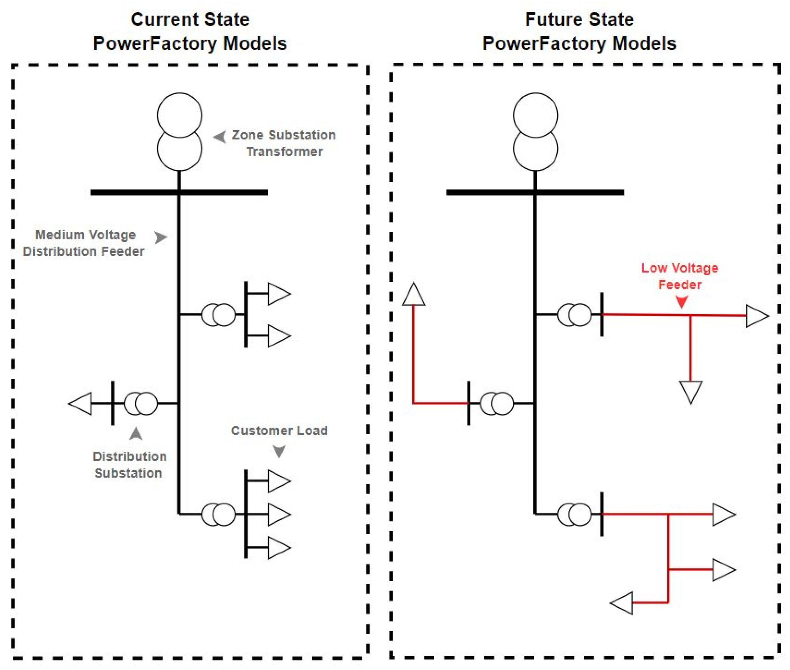
Prior to the uptake of solar PV systems, LV networks were not essential for traditional network planning studies, and as a result, information regarding the construction of these networks is often incomplete. Energy Queensland’s distribution networks models in DIgSILENT PowerFactory do not include the LV conductors.
The LV portion of the network is critical for modeling the effects of the customers’ PVs, as inverters control their active and reactive power outputs based on the voltages seen at the inverter terminals. The proposed research looks to expand the distribution network models to include the LV networks, as seen in
Figure 3 so that a realistic analysis can be conducted.
Two methods are utilized for constructing LV networks in DIgSILENT PowerFactory for the purpose of analysis. For each LV network, an attempt is made to construct actual models, i.e., genuine representations of the real network. If the data are incomplete or insufficient, i.e., missing conductor type information, load-flow analyses cannot be performed, and, therefore, representative networks are constructed in place of the actual.
3.1. Actual Networks
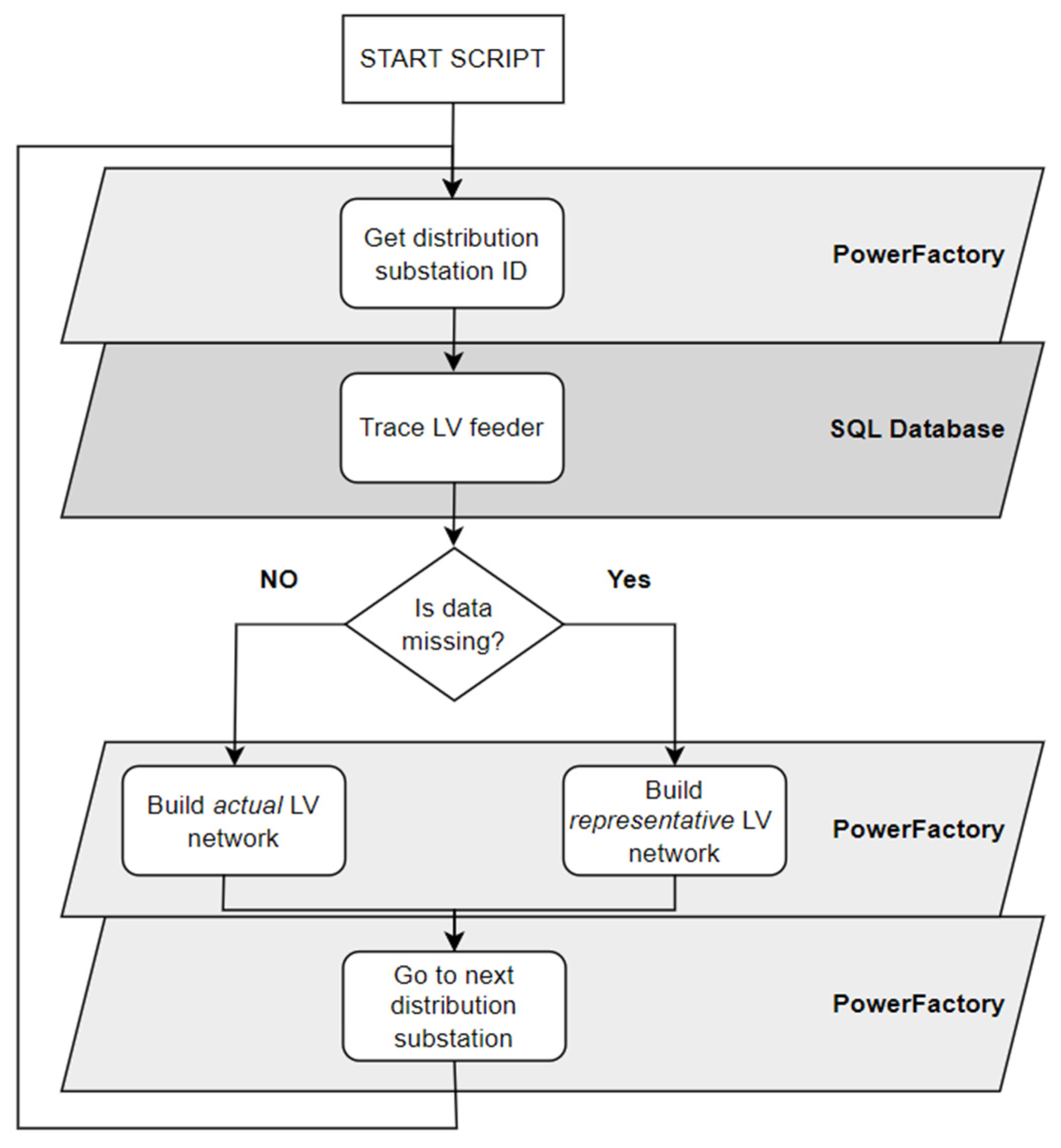
The project initially looked to create actual LV networks by programmatically tracing the Smallworld geospatial database. The term ‘actual’ means replicating networks as they appear in the GIS program Smallworld, which is reflective of real-world networks. For this task, a Python script was developed, which, when run in DIgSILENT PowerFactory, goes through each distribution substation and collects the substation ID, which is in the substation element’s name. With the ID collected, the GIS database is queried for the structural object related to that substation (either pole or padmount). The Smallworld database is then queried for the line object(s) (wire or cables) connected to that structural object. This process is repeated using a recursive programming technique until the trace reaches either the end of the line, an open point, or another distribution transformer, as illustrated in
Figure 4.
As mentioned in
Section 2.2, a major problem is the lack of quality data concerning LV networks, which means that actual networks cannot always be created. Common problems include missing conductor types and the reliability of network open points.
3.2. Representative Networks
Due to the challenges detailed in
Section 3.1, this research looked to build representative LV networks when actual networks could not be created.
The script developed for modeling the representative networks, when run in DIgSILENT PowerFactory, goes through each distribution substation and collects the substation ID, transformer size, and number of LV phases. With the ID collected, a number of corporate databases are queried to obtain information such as the number of connected customers and the feeder planning classification, urban or rural.
Using the transformer capacity and planning category, the LV network is matched to one of the representative models detailed in
Table 1 and
Table 2 in
Section 2.2. The network is made more accurate by using the actual number of customers and extending the length of the line if the number of customers exceeds the line length, given a specified number of customers per pole and distance between poles.
3.3. DIgSILENT PowerFactory Network Automation
Using the Python PowerFactory application interface (API), a script is used to automate the construction of the LV networks.
This process is as follows for each distribution transformer:
The substation ID is attained, which is the string of numbers in the first part of the substation element name;
The substation ID is used as the argument, i.e., input, to trace the LV network in the Smallworld database and obtain substation details, such as the number of customers and number of existing PV installations;
The traced network is analyzed for completeness by checking if there are any unknown conductor types;
If the data are complete, the actual networks are constructed in DIgSILENT PowerFactory; otherwise, representative networks are used.
This process is illustrated in
Figure 5.
Figure 6 shows the DIgSILENT PowerFactory application while the networks are being constructed. The output window at the bottom of the screen lists each of the networks as they are being created. The network model at the top of the screen shows the distribution network overview, and each of the circular objects is a distribution transformer; the two colors represent two different distribution feeders. The LV networks are not visible in this graphic but appear once a distribution substation is clicked on, which opens the internal view.
Figure 7 and
Figure 8 display a distribution transformer with a single customer on DIgSILENT PowerFactory, both before and after the LV network was created, respectively. The original load has been switched out of service on the transformer’s LV bus. To the left, three additional buses can be seen; the bus on the far left is a typical pole with a MEN; the next bus represents the attachment point on the house, and the final bus represents the end of a customer mains from the point of attachment to the switchboard; the load is now located there along with an earth stake and an inverter. The inverter is in service but may be switched in or out during the analysis phase if required, as this customer may or may not be forecast to have a PV inverter. The model is again equipped with line coupling to more accurately model the overhead phase and neutral wires.
4. Proposed Methodology for Network Analysis
With the LV networks on each distribution transformer constructed along each of the feeders in a DIgSILENT PowerFactory regional model, the analysis of each distribution feeder can begin.
The methodology for the analysis is as follows:
The forecasting database is queried for the number of PV systems and minimum underlying load for each year between 2020 and 2060 for each feeder;
The minimum load is applied to the feeder, and a load flow is conducted with feeder load scaling switched on;
Each load element is set to the resulting P and Q values, and feeder load scaling is switched off. This step allows the customers to determine the feeder load, as opposed to having the feeder converge to a specified value;
The number of PV systems forecast for that year are switched into service across a random distribution on the feeder. Each PV system is created with a QDSL model for fixed power factor and volt/var and volt/watt schemes. If the year is 2020, the inverters’ fixed power factor model is activated. For every year after, activated inverters have the volt/var and volt/watt models activated. Each PV system is set to have a rated output of 5 kVA to simulate a maximum generation, i.e., the worst-case scenario;
A load flow is conducted with feeder load scaling switched off;
Data points across the network are recorded;
Steps 1–6 are repeated for each year studied (2020–2060), changing the minimum load and activating additional PV systems as per the forecast;
The data are exported for further analysis.
The above process is illustrated in
Figure 9.
Quasi Dynamic Simulation Solar PV Modeling
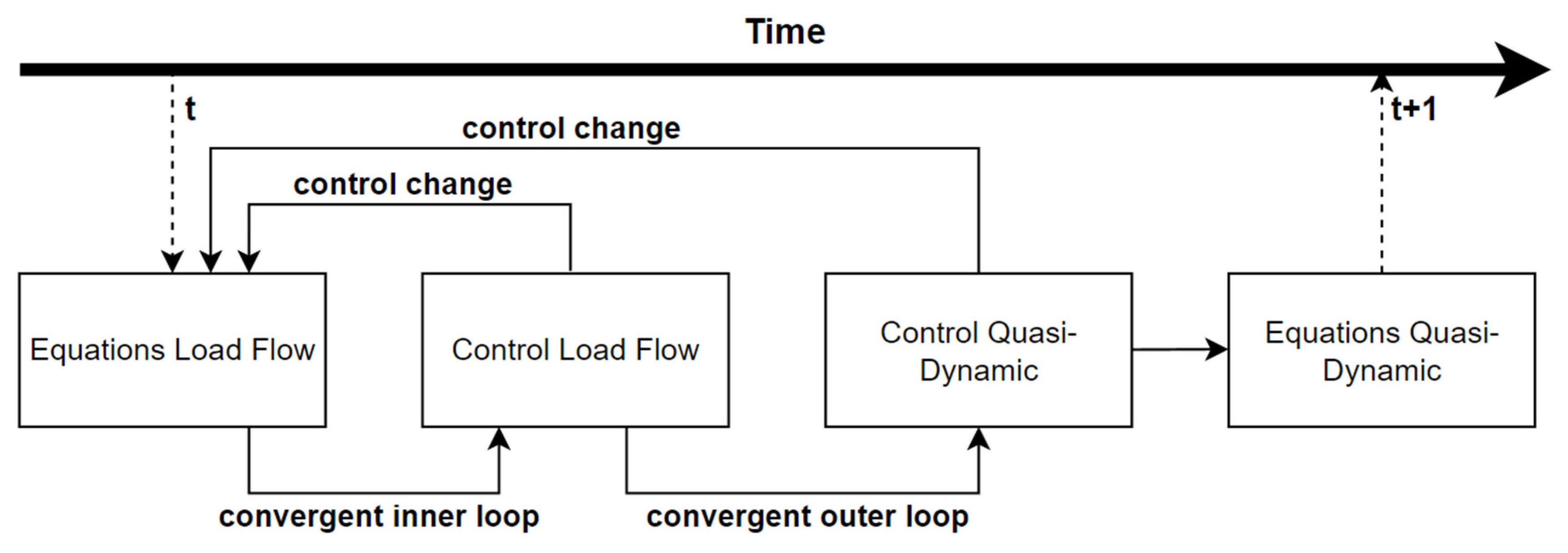
Each solar PV element activated in DIgSILENT PowerFactory is equipped with a QDSL element, which allows the inverters to dynamically control active and reactive power outputs as a function of the network voltage input. QDSL simulations achieve this through additional control loops after each time step, which are customizable through a series of parameters, equations, and logic scrips, as illustrated in
Figure 10.
An example of how this is applied to PV models is shown in
Figure 11 and
Figure 12.
Figure 11 displays the voltage and active and reactive power reference points that are used in the load flow outer loop script in
Figure 12 to calculate the inverters’ active and reactive power setpoints.
5. Results
Using a single distribution feeder at Boldon Hill, Qld, Australia as an example, the following plots illustrate the results of the forecast analysis, illustrating how the PV systems on the feeder respond to network voltage.
Figure 13 illustrates the voltage seen at each inverter’s terminals; as the forecast number of PV systems increases each year, so does the average voltage. This result confirms the theoretical principle that increasing energy generation on a system will result in an increase in system voltage. There are more data points each year as the forecast number of PV systems on the feeder increase.
Figure 14 and
Figure 15 illustrate the inverters’ active and reactive power output. Since every inverter in the year 2020 is set with a fixed power factor of 0.9, the active and reactive power output of every PV system in service that year is between 4.5 kW and −2.17 kvar, respectively.
For years after 2020, the volt–var and volt–watt responses are evident from the curtailment of active power and reactive power absorption experienced by some inverters, which is a result of the voltage levels at the connection point of those inverters.
Figure 14 shows that a few of the solar PV systems begin to curtail their active power output in 2029, and by 2048, they have completely curtailed to 1 kW, or 20% rated output, as described in AS4777 [
5] when the network voltage exceeds 260 V. These particular systems curtailing more heavily than the rest would indicate that they are either on a highly resistive section of the network, which would be more susceptible to voltage rise, or they are on the same LV network, and the effects of exporting energy are compounding.
It is to be noted that the aforementioned results are based on a combination of representative and actual networks and forecast input data. Accordingly, by aggregating the results across many feeders, appropriate trends can be determined.
5.1. Active Power Response on Distribution Feeders
Several zone substations and distribution feeders have been analyzed. The feeders are categorized into the planning categories of urban and rural to compare similar feeders, as the construction of urban and rural feeders vary significantly at both the MV and LV levels. The number of PV systems is used to compare feeders of various sizes as opposed to years.
5.1.1. Urban Feeder
Looking at the MV distribution feeder level,
Figure 16 illustrates the relationship between the number of PV systems and the minimum active power levels on urban feeders. It can be observed that with almost all feeders studied, as the number of PV systems is increased across years, the active power flows on the feeder are reversed, resulting in a net export of active power from the feeder into the substation.
The
x-axis in
Figure 16 represents the number of PV systems on each distribution feeder for each of the years analyzed. The
y-axis represents the active power seen by each distribution feeder in MW under minimum forecast load and influenced by the distributed PV generation. The legend shows each distribution feeder analyzed, represented by the different colors on the graph.
Using linear regression, a general rule for urban feeder active power as a function of the number of PV installations can be determined, as illustrated in
Figure 17.
The linear regression equation for the trend line is as follows:
The formula is in the format y = mx + c, where:
y is the feeder’s active power in kW;
m is the gradient (−3.42);
x is the number of PV systems installed on the feeder;
c is the y crossing, which in this case, is approximately 324 kW.
5.1.2. Rural Feeder
A similar trend, as seen on urban feeders, has been found for rural feeders, as seen in
Figure 18 and
Figure 19; whereas the number of PV systems increases during times of low load and high generation, the feeders’ net load becomes negative, meaning that they inject active power back into the substation.
The linear regression equation which represents the minimum active power levels on rural distribution feeders with a number of PV systems is:
5.2. Reactive Power Response on Distribution Feeders
By subtracting resulting levels of reactive power from the forecast underlying reactive power at each time step, we can determine the PV systems’ reactive power contribution to the feeder.
5.2.1. Urban Feeders
Figure 20 illustrates a decrease in the level of reactive power on distribution feeders as the number of PV systems increases. This response is indicative of the inverter’s volt/var control, where reactive power absorption is used to lower the voltage at the inverter terminals.
The linear regression equation, which represents the minimum reactive power levels on urban distribution feeders with a number of PV systems, as represented by the trend line in
Figure 21, is
5.2.2. Rural Feeders
Looking at the reactive power contribution of PVs to rural feeders, as shown in
Figure 22, and the trend for rural feeder reactive power, as shown in
Figure 23, it can be seen that the rate of decrease in reactive power is greater than that of urban feeders, which is expected as rural networks are often longer and built for less capacity which would make them more susceptible to the effects of PV generation.
The linear regression equation, which represents the minimum reactive power levels on rural distribution feeders with the number of PV systems, is
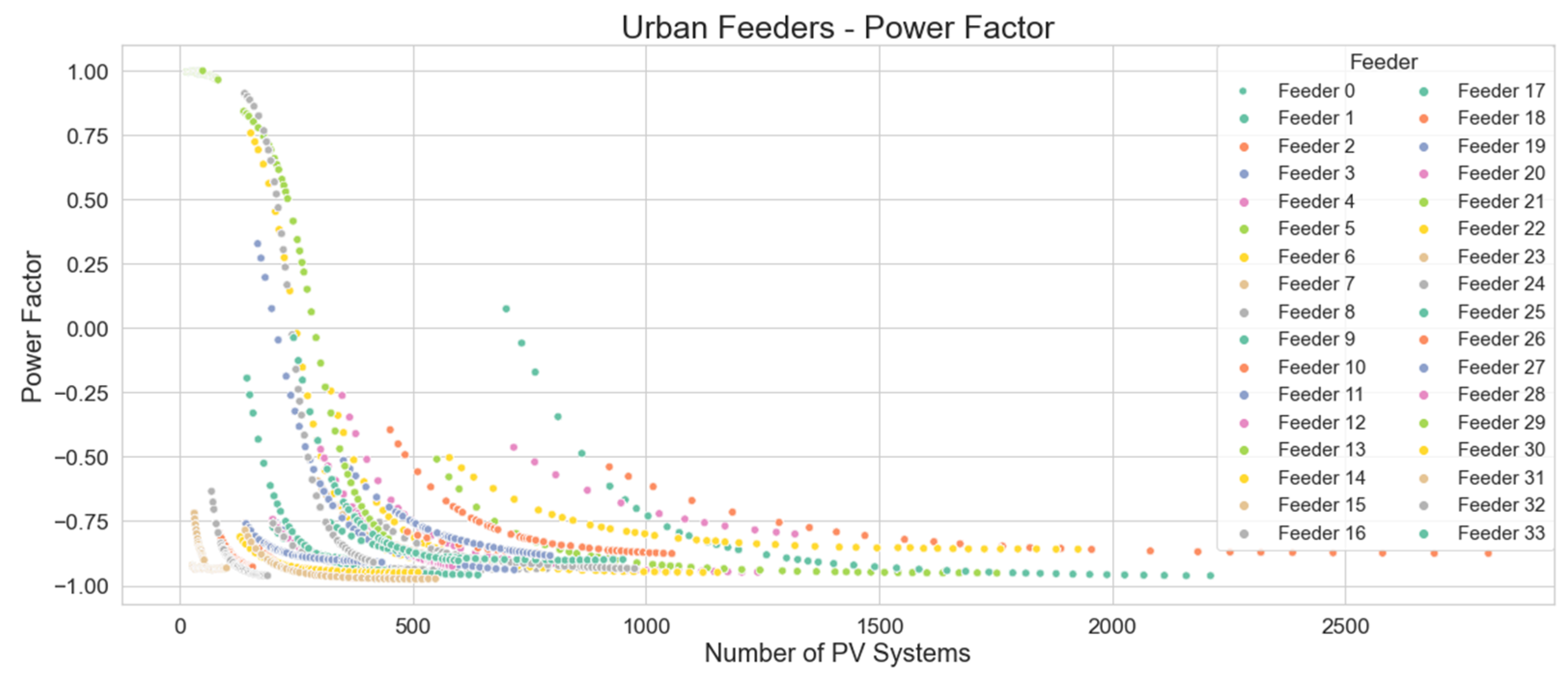
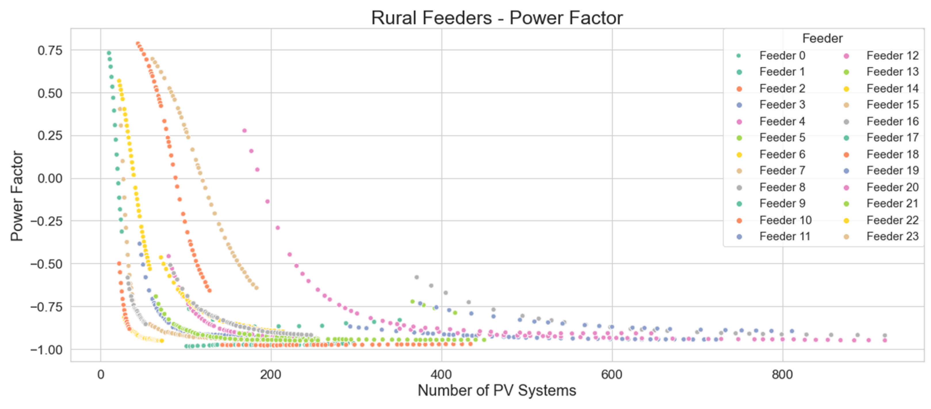
5.3. Effect of PV Systems on Distribution Feeder Power Factor
Figure 24 and
Figure 25 illustrate the effect of PV systems on urban and rural feeders, respectively. The power factor in each plot shows a shift from positive to negative values as the flow of power reverses.
5.4. Summary of Results
Table 4 details the trend equations for the relationship between solar PV connections and feeder power flow, where “y” is the power of MW or Mvar, and “x” is the number of PV systems connected to the feeder.
As highlighted in
Section 5.3, as solar PV generation increases and the active power flowing into the feeder from the wider network decreases, the power factor also decreases due to a change in the ratio between active and reactive power. Feeders experience a power factor close to zero when solar PV generation is in balance with the feeder load. This is because when no active power is flowing in or out of a feeder, reactive power flow is all that remains.
6. Discussion and Conclusions
A major concern for utility network planners is quantifying and managing the effects that increasing levels of rooftop solar PV has on distribution networks. The object of the research was twofold; to design a way to complete Energy Queensland’s network models in PowerFactory by adding LV feeders and, use these models to analyze forecast levels of customer load and rooftop PV.
Due to issues in the quality of LV network data, modeling and analyzing actual LV networks was not always achievable, and therefore, a combination of actual and representative models was used in this paper. The proposed research verified that clustering LV networks into representative models for the use of PV analysis can yield results with a high degree of accuracy compared to the actual network analysis.
Using the proposed approach, several of Energy Queensland’s distribution feeders were analyzed, and the results were grouped into the feeder’s planning category of urban or rural to compare feeders of similar network construction and topology. Comparing the number of installed solar PV systems for each distribution feeder with values measured at the feeder terminal, such as active power and reactive power, revealed pronounced trends between the feeders of a similar category.
Using linear regression, trends were determined, thus creating a simple metric by which to determine the network characteristics for other feeders with various levels of solar PV penetration. This estimation can easily be used as a rough guide for planning engineers to determine worst-case (minimum load) levels of power and voltage on distribution feeders in the future. Applying the tools developed in this research will save network planners time when forecasting network conditions by removing the need for detailed network modeling and analysis.
The power factor analysis raises the question of whether current standards reflect the reality of LV networks and whether or not network power factor statutory limits apply during periods of low load. Most network operators’ performance standards specify a power factor operating range from around 0.9 lagging to 0.9 leading.
In addition to satisfying the objectives, the proposed research delivered the ability to automate the creation of LV networks into Energy Queensland’s regional models, which is a tool that the organization can use in the future to analyze distribution networks in more detail. Use cases include assessing the hosting capacity of specific LV networks, assessing IES and load connections, and assessing EV charging and vehicle-to-grid impacts.
In future work, a methodology needs to be developed which seeks to formulate similar trends for varying network constructions and connection of standards/practices. This will provide broad benefits to network planners beyond Queensland, Australia. Furthermore, the results from this research should be compared with actual measurements in the future to verify forecast accuracy.
Author Contributions
Conceptualization, J.A. and A.P.A.; methodology, J.A.; software, J.A.; validation, J.A. and A.P.A.; formal analysis, J.A.; investigation, J.A.; resources, J.A.; data curation, J.A.; writing—original draft preparation, J.A.; writing—review and editing, A.P.A. and J.A.; visualization, J.A.; supervision, A.P.A.; project administration, A.P.A. All authors have read and agreed to the published version of the manuscript.
Funding
This research received no external funding.
Data Availability Statement
This study did not report any data.
Acknowledgments
The authors would like to thank the colleagues at Energy Queensland whose past work has set a foundation for this research.
Conflicts of Interest
The authors declare that they have no known competing financial interests or personal relationships that could have appeared to influence the work reported in this article.
References
- Wilkinson, S.; John, M.; Morrison, G. Rooftop PV and the Renewable Energy Transition a Review of Driving Forces and Analytical Frameworks. Sustainability 2021, 13, 5613. [Google Scholar] [CrossRef]
- Australians Install Record Amounts of Rooftop Solar Despite Lockdown, Supply Chain Pressures. Available online: https://www.abc.net.au/news/rural/2022-02-08/record-amounts-of-rooftop-solar-installed-during-lockdown/100805838 (accessed on 20 November 2022).
- Cheng, D.; Mather, B.A.; Seguin, R.; Hambrick, J.; Broadwater, R.P. Photovoltaic (PV) Impact Assessment for Very High Penetration Levels. IEEE J. Photovolt. 2016, 6, 295–300. [Google Scholar] [CrossRef]
- Mc Phail, D. Strategy for Addressing Impacts from Widespread Connection of Inverter Energy Systems; Ergon Energy: Townsville, Australia, 2011. [Google Scholar]
- AS/NZS 4777.2:2020; Grid Connection of ENERGY Systems via Inverters Inverter Requirements. Standards Australia: Sydney, Australia, 2020. Available online: https://infostore.saiglobal.com/en-us/standards/as-nzs-4777-2-2020-101208_saig_as_as_2906527/ (accessed on 27 July 2022).
- Tonkoski, R.; Lopes, L.C.; El-Fouly, T.M. Coordinated active power curtailment of grid connected PV inverters for overvoltage prevention. IEEE Trans. Sustain. Energy 2011, 2, 139–147. [Google Scholar] [CrossRef]
- Umoh, V.; Davidson, I.; Adebiyi, A.; Ekpe, U. Methods and Tools for PV and EV Hosting Capacity Determination in Low Voltage Distribution Networks—A Review. Energies 2023, 16, 3609. [Google Scholar] [CrossRef]
- Kawamura, H.; Sano, E.A. Congestion control system for an advanced intelligent network. In Proceedings of the NOMS ′96—IEEE Network Operations and Management Symposium, Kyoto, Japan, 15–19 April 1996; Volume 2, pp. 628–631. [Google Scholar]
- Australian Energy Market Operator 2022—Integrated System Plan. Available online: https://aemo.com.au/en/energy-systems/major-publications/integrated-system-plan-isp/2022-integrated-system-plan-isp (accessed on 20 June 2022).
- Navarro, B.B.; Navarro, M.M. A comprehensive solar PV hosting capacity in MV and LV radial distribution networks. In Proceedings of the IEEE PES Innovative Smart Grid Technologies Conference Europe (ISGT-Europe), Torino, Italy, 26–29 September 2017; Volume 225, pp. 1–6. [Google Scholar]
- Liu, Y.; Bebic, J.; Kroposki, B.; de Bedout, J.; Ren, W. Distribution system voltage performance analysis for high-penetration PV. In Proceedings of the IEEE Energy 2030 Conference, Atlanta, Georgia, 17–18 November 2008; Volume 1, pp. 1–8. [Google Scholar]
- O’Shaughnessy, E.; Cruce, J.; Xu, K. Too much of a good thing? global trends in the curtailment of solar PV. Solar Energy 2020, 208, 1068–1077. [Google Scholar] [CrossRef] [PubMed]
- Samuel, A.T.; Aldamanhori, A.; Ravikumar, A.; Konstantinou, G. Stochastic modeling for future scenarios of the 2040 Australian national electricity market using ANTATES. In Proceedings of the International Conference on Smart Grids and Energy Systems (SGES), Perth, Australia, 23–26 November 2020; Volume 128, pp. 761–766. [Google Scholar]
- Chathurangi, D.; Jayatunga, U.; Rathnayake, M.; Wickramasinghe, A.; Agalgaonkar, A.; Perera, S. Potential power quality impacts on lv distribution networks with high penetration levels of solar PV. In Proceedings of the 18th International Conference on Harmonics and Quality of Power (ICHQP), Ljubljana, Slovenia, 13–16 May 2018; Volume 18, pp. 1–6. [Google Scholar]
- Rigoni, V.; Ochoa, R.F.; Chicco, G.; Navarro-Espinosa, A.; Gozel, T. Representative Residential LV Feeders: A case study for the North West of England. IEEE Trans. Power Syst. 2015, 31, 348–360. [Google Scholar] [CrossRef]
- Chathurangi, D.; Jayatunga, U.; Perera, S.; Agalgaonkar, A.; Siyambalapitiya, T.; Wickramasinghe, A. Connection of Solar PV to lv Networks: CONSIDERATIONS for Maximum Penetration Level; AUPEC: Auckland, New Zealand, 2018; Volume 12, pp. 1–6. [Google Scholar]
- Eguia, P.; Etxegarai, A.; Torres, E.; San Martin, J.I.; Albizu, I. Modeling and validation of photovoltaic plants using generic dynamic models. In Proceedings of the International Conference on Clean Electrical Power (ICCEP), Taormina, Italy, 16–18 June 2015; Volume 255, pp. 78–84. [Google Scholar]
- Rashid, M.; Knight, A.M. Combining volt/var volt/watt modes to increase PV hosting capacity in lv distribution networks. In Proceedings of the IEEE Electric Power and Energy Conference (EPEC), Edmonton, AB, Canada, 9–10 November 2020; Volume 19, pp. 1–5. [Google Scholar]
- Maduranga, R.; Maddumage, M.; Kaushalya, P.; Samith, D.; Jayatunga, U. Investigation of grid connected solar PV hosting capacity in lv distribution networks. In Proceedings of the 14th Conference on Industrial and Information Systems (ICIIS), Kandy, Sri Lanka, 18–20 December 2019; Volume 129, pp. 390–394. [Google Scholar]
- DIgSILENT Powerfactory 2020: User Manual. Available online: https://www.digsilent.de/en/downloads.html (accessed on 11 May 2022).
- A Quasi-Dynamic Approach for Slow Dynamics Time Domain Analysis of Electrical Networks with Distributed Energy Resources. Available online: https://www.researchgate.net/publication/310301463_A_quasi-dynamic_approach_for_slow_dynamics_time_domain_analysis_of_electrical_networks_with_distributed_energy_ressources (accessed on 15 March 2022).
- Raza, M.Q.; Nadarajah, M.; Ekanayake, C. On recent advances in PV output power forecast. Solar Energy 2016, 136, 125–144. [Google Scholar] [CrossRef]
- Collares-Pereira, M.; Rabl, A. The average distribution of solar radiation-correlations between diffuse and hemispherical and between daily and hourly insolation values. Solar Energy 1979, 22, 155–164. [Google Scholar] [CrossRef]
- Maxwell, E.L. METSTAT—The solar radiation model used in the production of the National Solar Radiation Data Base (NSRDB). Solar Energy 1998, 62, 263–276. [Google Scholar] [CrossRef]
- Yang, D. Choice of clear-sky model in solar forecasting. Renew. Sustain. Energy 2020, 12, 101–109. [Google Scholar] [CrossRef]
- Marquez, R.; Coimbra, C.F. Intra-hour DNI forecasting based on cloud tracking image analysis. Solar Energy 2013, 91, 327–336. [Google Scholar] [CrossRef]
- Chow, C.W.; Urquhart, B.; Lave, M.; Dominguez, A.; Kleissl, J.; Shields, J.; Washom, B. Intra-hour forecasting with a total sky imager at the UC San Diego solar energy testbed. Solar. Energy 2011, 85, 2881–2893. [Google Scholar] [CrossRef]
- Zhen, Z.; Wang, F.; Mi, Z.; Sun, Y.; Sun, H. Cloud Tracking and Forecasting Method Based on Optimization Model for PV Power Forecasting; AUPEC: Auckland, New Zealand, 2015; Volume 55, pp. 1–4. [Google Scholar]
- Zamo, M.; Mestre, O.; Arbogast, P.; Pannekoucke, O. A benchmark of statistical regression methods for short-term forecasting of photovoltaic electricity production, Part I: Deterministic forecast of hourly production. Solar. Energy 2014, 105, 792–803. [Google Scholar] [CrossRef]
- Mokhtar, M.; Robu, V.; Flynn, D.; Higgins, C.; Whyte, J.; Loughran, C.; Fulton, F. Predicting the voltage distribution for low voltage networks using deep learning. In Proceedings of the IEEE PES Innovative Smart Grid Technologies Europe (ISGT-Europe), Torino, Italy, 26–29 September 2017; Volume 39, pp. 1–5. [Google Scholar]
- Shao, C.; Feng, C.; Zhang, X.; Tang, H.; Liu, J. Optimization method based on load forecasting for three-phase imbalance mitigation in low-voltage distribution network. In Proceedings of the IEEE 5th International Electrical and Energy Conference (CIEEC), Nanjing, China, 27–29 May 2022; Volume 335, pp. 1032–1037. [Google Scholar]
- Energy Queensland 2022 Strategic Annual Forecasting Report. Available online: https://www.energex.com.au/__data/assets/pdf_file/0016/340603/STNW1170-Connection-Standard-for-Micro-EG-Units.pdf (accessed on 26 April 2022).
- STNW1170 Standard for Small IES Connections. Available online: https://www.energex.com.au/__data/assets/pdf_file/0016/340603/STNW1170-Standard-for-Small-IES-Connections.pdf (accessed on 15 March 2022).
Figure 1.
Energy Queensland’s micro-embedded generation volt–var connection requirement [
33].
Figure 1.
Energy Queensland’s micro-embedded generation volt–var connection requirement [
33].
Figure 2.
Energy Queensland’s micro-embedded generation volt–watt connection requirement [
33].
Figure 2.
Energy Queensland’s micro-embedded generation volt–watt connection requirement [
33].
Figure 3.
LV network modeling.
Figure 3.
LV network modeling.
Figure 4.
LV network tracing process.
Figure 4.
LV network tracing process.
Figure 5.
Constructing LV networks script flowchart.
Figure 5.
Constructing LV networks script flowchart.
Figure 6.
Constructing LV networks in DIgSILENT PowerFactory.
Figure 6.
Constructing LV networks in DIgSILENT PowerFactory.
Figure 7.
DIgSILENT PowerFactory distribution transformer model before LV network creation.
Figure 7.
DIgSILENT PowerFactory distribution transformer model before LV network creation.
Figure 8.
DIgSILENT PowerFactory distribution transformer model after LV network creation.
Figure 8.
DIgSILENT PowerFactory distribution transformer model after LV network creation.
Figure 9.
Network analysis script flowchart.
Figure 9.
Network analysis script flowchart.
Figure 10.
DIgSILENT PowerFactory QDSL models—Simulation Procedure.
Figure 10.
DIgSILENT PowerFactory QDSL models—Simulation Procedure.
Figure 11.
DIgSILENT PowerFactory QDSL element volt–var and volt–watt parameters.
Figure 11.
DIgSILENT PowerFactory QDSL element volt–var and volt–watt parameters.
Figure 12.
DIgSILENT PowerFactory QDSL element volt–var and volt–watt load flow script.
Figure 12.
DIgSILENT PowerFactory QDSL element volt–var and volt–watt load flow script.
Figure 13.
Bolden Hill distribution feeder—PV system voltage.
Figure 13.
Bolden Hill distribution feeder—PV system voltage.
Figure 14.
Bolden Hill distribution feeder—PV system active power output.
Figure 14.
Bolden Hill distribution feeder—PV system active power output.
Figure 15.
Bolden Hill distribution feeder—PV system reactive power response.
Figure 15.
Bolden Hill distribution feeder—PV system reactive power response.
Figure 16.
Urban distribution feeders’ minimum active power level.
Figure 16.
Urban distribution feeders’ minimum active power level.
Figure 17.
Urban distribution feeders’ minimum active power level—trend line.
Figure 17.
Urban distribution feeders’ minimum active power level—trend line.
Figure 18.
Rural distribution feeders’ minimum active power level.
Figure 18.
Rural distribution feeders’ minimum active power level.
Figure 19.
Rural distribution feeders’ minimum active power level—trend line.
Figure 19.
Rural distribution feeders’ minimum active power level—trend line.
Figure 20.
Urban distribution feeders’ reactive power contribution from PV.
Figure 20.
Urban distribution feeders’ reactive power contribution from PV.
Figure 21.
Urban distribution feeders’ reactive power contribution from PV—trend line.
Figure 21.
Urban distribution feeders’ reactive power contribution from PV—trend line.
Figure 22.
Rural distribution feeders’ reactive power contribution from PV.
Figure 22.
Rural distribution feeders’ reactive power contribution from PV.
Figure 23.
Rural distribution feeders reactive power contribution from PV—trend line.
Figure 23.
Rural distribution feeders reactive power contribution from PV—trend line.
Figure 24.
Variation in power factor on urban distribution feeders.
Figure 24.
Variation in power factor on urban distribution feeders.
Figure 25.
Variation in power factor on rural distribution feeders.
Figure 25.
Variation in power factor on rural distribution feeders.
Table 1.
Energy Queensland’s typical LV network construction.
Table 1.
Energy Queensland’s typical LV network construction.
Feeder
Category | TF Size (kVA) | No. of Customers | Conductor Type | Length | Type |
|---|
| Urban | 10 (1 ph) | 2 | 2 × 25 mm2 ABC | 60 m | Overhead |
| Urban | 25 | 3 | 2 × 95 mm2 ABC | 100 m | Overhead |
| Urban | 50 | 7 | 4 × 95 mm2 ABC | 350 m | Overhead |
| Urban | 50 | 8 | 120 mm2 Al 1C XLPE | 300 m | Underground |
| Urban | 63 | 5 | 4 × 95 mm2 ABC | 250 m | Overhead |
| Urban | 100 | 20 | 4 × 95 mm2 ABC | 370 m | Overhead |
| Urban | 100 | 20 | 120 mm2 Al 1C XLPE | 130 m | Underground |
| Urban | 200 | 44 | Mars 7/3.75 AAC | 250 m | Overhead |
| Urban | 315 | 38 | Mars 7/3.75 AAC | 350 m | Overhead |
| Urban | 315 | 38 | 240 mm2 Al 4C XLPE | 250 m | Underground |
| Urban | 500 | 38 | 240 mm2 Al 4C XLPE | 300 m | Underground |
| Rural | 10 | 1 | 2 × 50 mm2 ABC | 75 m | Overhead |
| Rural | 25 | 2 | 4 × 95 mm2 ABC | 120 m | Overhead |
| Rural | 50 | 4 | 4 × 95 mm2 ABC | 250 m | Overhead |
| Rural | 63 | 3 | 4 × 95 mm2 ABC | 120 m | Overhead |
| Rural | 100 | 7 | Mars 7/3.75 AAC | 300 m | Overhead |
| Rural | 200 | 14 | 4 × 95 mm2 ABC | 400 m | Overhead |
Table 2.
Additional assumptions for Energy Queensland’s LV networks.
Table 2.
Additional assumptions for Energy Queensland’s LV networks.
| Element | Urban | Rural |
|---|
| MEN resistance | 10 Ω | 1 Ω |
| Transformer earth resistance | 10 Ω | 1 Ω |
| Customer earth stake resistance | 10 Ω | 10 Ω |
| Distance between poles | 15 m | 50 m |
| Customer service * length | 15 m | 30 m |
| Customer service conductor type | 25 mm2 Al | 16 mm2 Al |
| Customer mains ** length | 15 m urban | 20 m |
| Customer mains conductor type | 10 mm2 CU | 10 mm2 CU |
Table 3.
Energy Queensland feeder forecast example.
Table 3.
Energy Queensland feeder forecast example.
| Forecast Year | Num PV Systems | Underlying kW | Underlying Kvar |
|---|
| 2020 | 169 | 845.7 | −60.9 |
| 2021 | 177 | 851.7 | −60.5 |
| 2022 | 184 | 856.8 | −60.2 |
| …. | | | |
| 2060 | 646 | 1779.2 | −42.0 |
Table 4.
Feeder PV and power flow trend equations.
Table 4.
Feeder PV and power flow trend equations.
| Feeder Type | Active Power Equation | Reactive Power Equation |
|---|
| Urban | y = −3.42x + 324.01 | y = −1.6x − 1.03 |
| Rural | y = −4.13x + 153.47 | y = −1.57x − 9.84 |
| Disclaimer/Publisher’s Note: The statements, opinions and data contained in all publications are solely those of the individual author(s) and contributor(s) and not of MDPI and/or the editor(s). MDPI and/or the editor(s) disclaim responsibility for any injury to people or property resulting from any ideas, methods, instructions or products referred to in the content. |
© 2023 by the authors. Licensee MDPI, Basel, Switzerland. This article is an open access article distributed under the terms and conditions of the Creative Commons Attribution (CC BY) license (https://creativecommons.org/licenses/by/4.0/).


