Stator ITSC Fault Diagnosis of EMU Asynchronous Traction Motor Based on apFFT Time-Shift Phase Difference Spectrum Correction and SVM

Abstract

EMU (electric multiple unit) traction motors are powered by converters whose output voltage increases the voltage stress borne by the insulation system, making the ITSC (inter-turn short-circuit) fault more prominent. An index based on short-circuit thermal power is proposed in the article to evaluate the non-metallic ITSC faults extent. The apFFT (all-phase FFT) time-shift phase difference correction with double Hanning windows is used to calculate fault features to train the SVM (support vector machine) fault diagnosis model whose hyper-parameters C and g are optimized using grid search methods. The experimental verification was carried out on the EMU electric traction simulation experimental platform. According to the fault extent index proposed in this article, the experimental samples were divided into three categories, normal, incipient and serious fault samples. The ITSC fault diagnosis accuracy was 100% on the training dataset and 93.33% on the test dataset. There was no misclassification between normal and serious ITSC fault samples.

1. Introduction

The AC–DC–AC transmission mode is used in modern EMU traction systems, and three-phase AC squirrel-cage asynchronous motors are used as traction motors [1]. Affected by mechanical stress, thermal stress, and electrical stress, EMU traction motors are prone to failure [2,3]. The fault types of three-phase AC asynchronous squirrel-cage motors in industrial applications mainly include stator insulation faults (37%), rotor broken bar faults (12%), bearing faults (41%), and other faults (10%) [4]. The high voltage stress generated by the inverter PWM (pulse width modulation) voltage accelerates the degradation of the traction motor insulation system [5,6,7,8]. The inter-turn insulation is the weakest part of the asynchronous traction motor insulation system [9]. When an ITSC fault occurs, an inter-turn current circulates between the short-circuit turns, quickly producing a large amount of heat [10], which weakens the insulation of the motor and results in inter-phase or ground short-circuit faults [11]. Timely maintenance can prevent the ITSC fault’s further expansion and significantly reduce the maintenance cost. Since the ITSC fault of the asynchronous traction motor is more hidden than the main insulation system fault, it is more difficult to detect the incipient ITSC fault [12,13].

The ITSC fault diagnosis of three-phase asynchronous motors mainly includes model-based, signal process–based, and artificial intelligence–based diagnosis methods [14,15,16]. An accurate motor ITSC fault model is needed for model-based ITSC fault diagnosis. Model-based methods mainly include the parameter estimation method and residual estimation method. With the parameter estimation method, the model parameters related to the ITSC fault are estimated [17,18,19]. Based on the three-phase asynchronous motor ITSC fault model under the dq axis, the particle filter algorithm is used to estimate multiple parameters to detect the stator ITSC fault and assess the motor insulation residual life [20]. With this method, real-time and non-intrusive diagnosis can be easily achieved by just measuring motor phase voltage and phase current. A healthy motor model is necessary for the residual estimation method, which takes the detectable variables related to the ITSC fault as state variables. It uses the difference between the state variables of the healthy motor estimated by the model and the measured variables as the residual to detect the ITSC fault [21,22]. The three-phase current is taken as the state variable, and the high-order sliding mode observer is used to observe the three-phase current of the healthy motor [23]. The residual of the observed and measured values is taken as the index for the ITSC fault. The model-based ITSC fault diagnosis method can be easily affected by working conditions. For example, when the method of estimating stator resistance is used to diagnose ITSC faults, the diagnostic results are highly influenced by temperature and frequency (skin effect).

The diagnosis method for the ITSC fault based on signal processing is mainly based on the electrical, magnetic, thermal, vibration, and acoustic signals. The stator ITSC fault is diagnosed by analyzing and processing the above signals in the time, frequency, or time–frequency domains [24,25,26]. The voltage or current signals can be used to realize non-intrusive diagnosis [27], saving costs without the need for installing extra sensors. For the steady operation state, the FFT algorithm is generally used to calculate specific frequency components of the current or other signals to detect the ITSC fault [28]. With the continuous development of new signal processing methods, time–frequency analysis methods, such as wavelet transform, WVD (Wigner–Ville distribution), and HHT (Hilbert–Huang transform), are also applied to the motors’ fault diagnosis [29,30]. The discrete wavelet is used to decompose the stator current, and the maximum norm of the detail coefficient is used to detect the incipient ITSC fault [31].

Shallow machine learning and deep learning methods are also applied to motor stator ITSC fault diagnosis [32,33,34,35]. The ITSC fault diagnosis method based on shallow machine learning is generally divided into three stages: data preparation, feature extraction, and model training. Particle swarm optimization and principal component analysis can be used for feature extraction. The BP neural network and SVM models can be used as diagnosis models. The BP neural network is trained based on the phase difference of the three-phase stator current, which can detect and locate the stator ITSC fault [36]. When a deep learning network is adopted, such as a convolution neural network, it is unnecessary to extract features artificially because the deep learning network automatically extracts them. The instantaneous value of the three-phase current is taken as the feature, the convolution neural network is taken as the diagnosis model, and the trained convolution neural network can accurately detect the ITSC fault of a three-phase asynchronous motor [37].

Research on the diagnosis method for ITSC fault of asynchronous motors stator has achieved many positive results, but the diagnosis of EMU traction motor stator ITSC fault has special needs. Firstly, in previous studies, the extent of an AC motor ITSC fault is generally evaluated based on the number of short-circuit turns when the inter-turn resistance is fixed. In the non-metallic short circuit, the resistance between short-circuit turns is directly related to the extent of the motor damage caused by the fault. Secondly, most of the previous studies are carried out in the condition of non-variable frequency speed regulation, and the steady speed of the motor is fixed. The traction motor operates stably at different speeds according to operating conditions. Finally, the traction motor of the EMU adopts vector control or direct torque control based on the current closed loop. The fundamental frequency of voltage and current signals cannot be directly obtained, and a spectral correction method is needed to achieve a more accurate fundamental frequency.

The article is mainly divided into five parts. After the introduction, it introduces the measurement method for the traction motor’s ZSVC (zero-sequence voltage component) and the apFFT time-shift phase difference correction method. This method is used to calculate the traction motor’s ZSVC fundamental frequency, the fundamental component amplitudes of the ZSVC and the three-phase current in a steady state. In the third part, an ITSC fault extent index related to the number of short-circuit turns and the inter-turn resistance is proposed. The index is based on the thermal power of the circulating current between short-circuit turns. In addition, the SVM and the hyper-parameter optimization method are introduced in this part. In the following section, SVM is used to diagnose the ITSC fault. The fourth part is the experimental part. The EMU electric traction simulation experimental platform is used to simulate the steady-state operation of the EMU. According to the fault extent index proposed in this article, the experimental samples are divided into normal, incipient, and serious fault samples, and the ITSC fault diagnosis model is trained and tested. The last part summarizes all the research contents and puts forward the follow-up work.

2. Calculation of Signals’ Fundamental Components

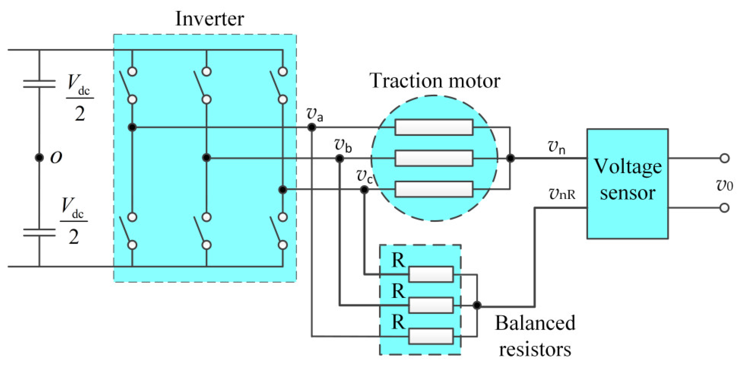
2.1. ZSVC Measurement Method

The traction motor’s current is measured for speed and torque control during the operation, and only the ZSVC needs to be measured additionally. The ZSVC of the three-phase asynchronous motor can effectively monitor the stator ITSC fault [38,39]. The measurement circuit is relatively simple, and installing sensors on the motor body is unnecessary. According to the ZSVC definition of a three-phase asynchronous motor [40,41], as shown in Formula (1), three voltage sensors are needed when measuring the three-phase voltage.

$$v_0=\frac{1}{3}\left(v_{\mathrm{an}}+v_{\mathrm{bn}}+v_{\mathrm{cn}}\right)$$

(1)

Directly measuring three-phase voltage and calculating ZSVC according to Formula (1) can be applied to a sinusoidal power supply. The EMU traction inverter generates the ZSVC inherent in the PWM voltage and related to the PWM modulation mode. Although the frequency produced by the inverter is far from the fundamental frequency, if reasonable compensation and filtering are not carried out, frequency aliasing occurs, and the measurement is affected. The ZSVC measurement of the traction motor in Figure 1 is adopted, wherein both v_n and v_nR contain the ZVSC produced by the inverter. v₀ is the difference between them and only contains the ZVSC caused by the stator ITSC fault and asymmetry, so the three balanced resistors can eliminate the influence of the inverter [42].

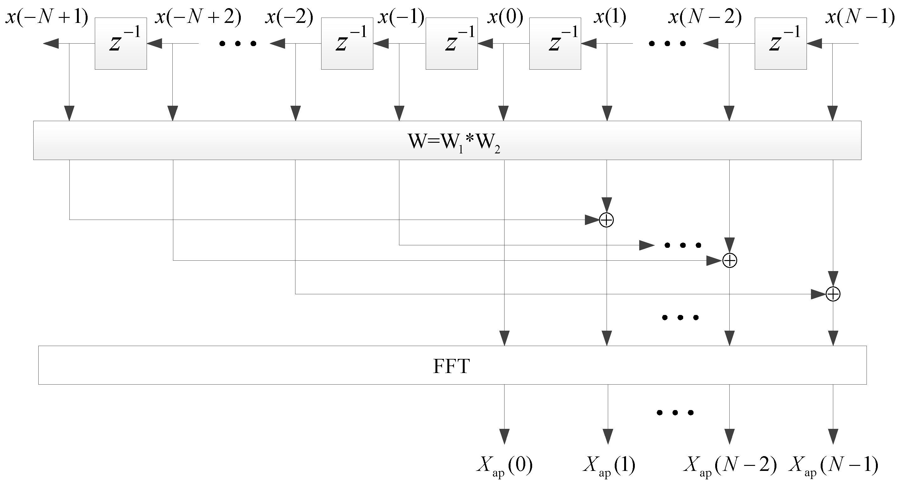
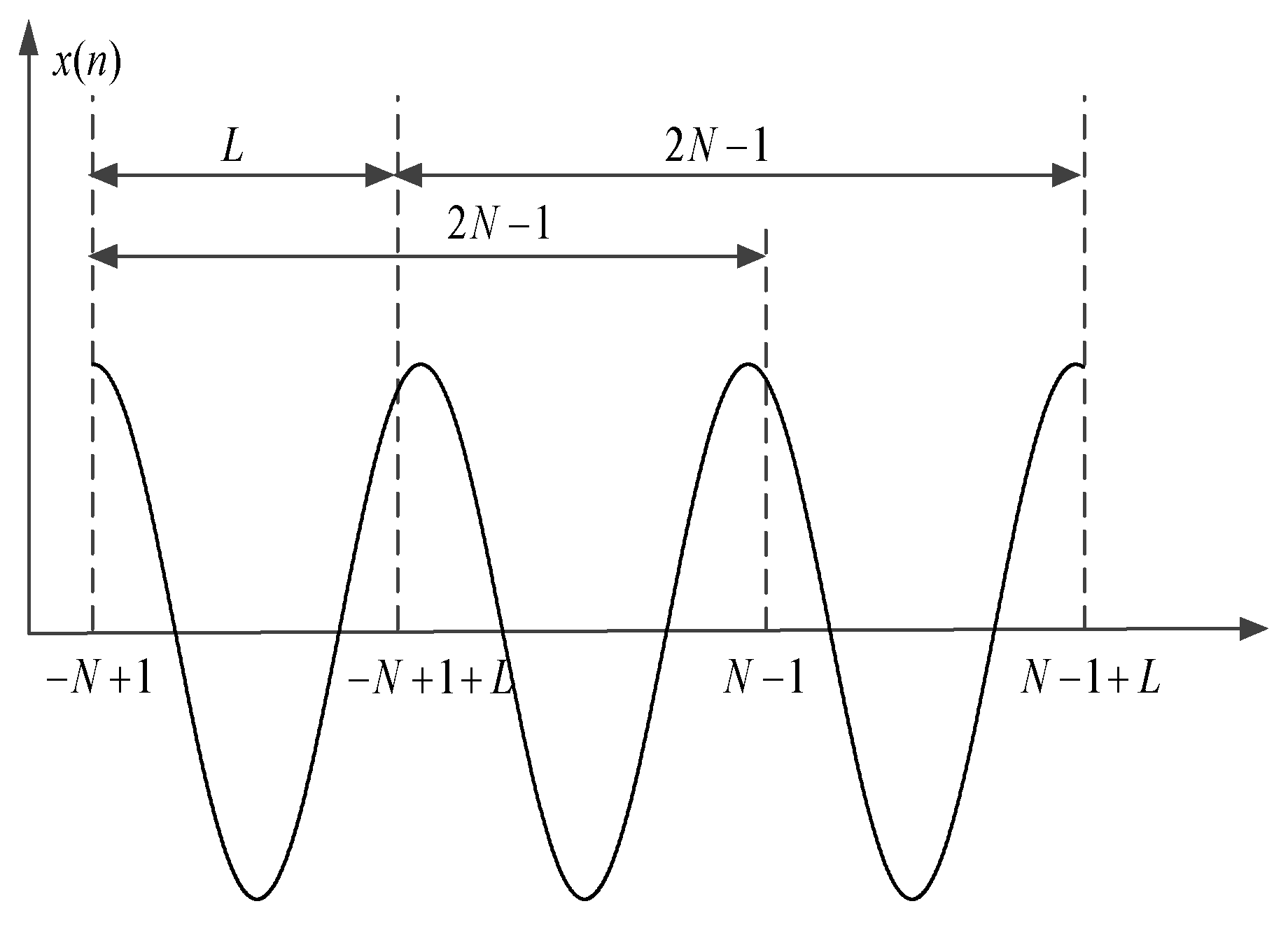
2.2. ApFFT Time-Shift Phase Difference Correction Algorithm

The apFFT time-shift phase difference correction mainly includes two parts, i.e., apFFT and time-shift phase difference correction. The apFFT algorithm can effectively suppress spectrum leakage caused by data truncation [43,44,45]. As shown in Figure 2, the required data points for the N-order spectrum analysis are x(−N + 1), x(−N + 2), …, x(−1), x(1), …, x(N − 2), x(N − 1) with a total of 2N − 1 data points. W is a convolution window formed by a convolution operation with the front window W₁ and the flipped rear window W₂. When both W₁ and W₂ are rectangular windows, the spectrum analysis approach is referred to as windowless apFFT. When either W₁ or W₂ is a rectangular window, the spectrum analysis approach is referred to as single-window apFFT. When neither W₁ nor W₂ is a rectangular window, the spectrum analysis approach is referred to as double-window apFFT.

The N-order apFFT spectrum analysis mainly includes the preprocessing of 2N − 1 point data and the FFT calculation. If the data are processed by windowless apFFT, the following operations can be performed on the data. First, divide 2N − 1 data points into N segments with length N according to Formula (2):

$$\begin{array}{c}{x}_0={[x(0),x(1),x(2),\dots ,x(N-1)]}^T,\\ x_1={[x(-1),x(0),x(1),\dots ,x(N-2)]}^T,\\ x_2={[x(-2),x(-1),x(0),\dots ,x(N-3)]}^T,\\ \dots \dots \\ x_{N-1}={[x(-N+1),x(-N+2),\dots ,x(0)]}^T.\end{array}$$

(2)

Then, rotate the N segment data of Formula (2), taking the Nth data point, i.e., x(0), as the first data point of the data segment. Formula (2) is transformed into Formula (3):

$$\begin{array}{c}{x}_0={[x(0),x(1),x(2),\dots ,x(N-1)]}^T,\\ x_1={[x(0),x(1),\dots ,x(N-2),x(-1)]}^T,\\ x_2={[x(0),\dots ,x(N-3),x(-2),x(-1)]}^T,\\ \dots \dots \\ x_{N-1}={[x(0),x(-N+1),\dots ,x(-2),x(-1)]}^T.\end{array}$$

(3)

Finally, add the shifted N segments of the data separately and normalize them to obtain x_ap in Formula (4), which comprises the N data points obtained after the windowless apFFT preprocessing.

$$x_{\mathrm{ap}}=\frac{1}{N}{[Nx(0),(N-1)x(1)+x(-N+1),\dots ,x(N-1)+(N-1)x(-1)]}^T.$$

(4)

Perform N-point FFT on x_ap; that is, obtain the calculation result X_ap(k) of windowless apFFT, and k is the spectrum index.

The second part of the apFFT time-shift phase difference correction algorithm is the time-shift phase difference correction [46]. The single-frequency complex exponential signal with frequency ω*, initial phase θ₀, and amplitude A is x(n), where n is the discrete time point.

$$x(n)=A{e}^{j(w^{\ast }n+{\theta }_0)},$$

(5)

The data points are divided into two segments of the same length, as shown in Figure 3. The data interval of the first segment is [−N + 1, N − 1]. Assuming the spectrum serial number is k*, the phase value of apFFT main spectrum line is:

$${\phi }_X(k^{\ast })={\theta }_0,$$

(6)

The second data segment starts after L data points of the first data segment. The data range is [−N + 1 + L, N − 1 + L]. The central data point of this data segment is x(−L), as shown in Figure 3. If apFFT is performed on the second segment of data, the phase of apFFT main spectral line is ${\phi }_{XL}(k^{\ast })$, which is the approximate estimation of the phase of data point x(−L); that is,

$${\phi }_{\mathrm{X}\mathrm{L}}(k^{\ast })={\theta }_0-{\omega }^{\ast }L,$$

(7)

The estimation of signal frequency can be obtained from Formulas (6) and (7):

$${\widehat{\omega }}^{\ast }=\left[{\phi }_X\left(k^{\ast }\right)-{\phi }_{XL}\left(k^{\ast }\right)\right]/L=\Delta \phi /L,$$

(8)

To eliminate the “phase ambiguity” phenomenon [47], the frequency estimation after phase compensation is [48]

$${\widehat{\omega }}^{\ast }=\left[{\phi }_X\left(k^{\ast }\right)-{\phi }_{XL}\left(k^{\ast }\right)\right]/L+2k^{\ast }\pi /N,$$

(9)

For the double-window apFFT, the signal amplitude estimation can be obtained:

$$\widehat{A}=\frac{\left|Y\left(k^{\ast }\right)\right|}{{\left|F_{\mathrm{g}}\left(k^{\ast }\Delta \omega -{\widehat{\omega }}^{\ast }\right)\right|}^2}.$$

(10)

In Equation (10), Y(k^*) is the value of the double-window apFFT at point k^*; $F_{\mathrm{g}}\left(k^{\ast }\Delta \omega -{\widehat{\omega }}^{\ast }\right)$ is obtained from bringing $\left(k^{\ast }\Delta \omega -{\widehat{\omega }}^{\ast }\right)$ into the Fourier transform of the window function. Generally, the window function is a cosine window, and its Fourier transform expression is determined.

3. Fault Diagnosis Method for Stator ITSC Fault of Traction Motor

3.1. Stator ITSC Fault Extent Index

In previous studies, only the metallic short circuit of windings is generally considered. The two windings are directly short-circuited without any resistance, and the motor’s ITSC fault extent is evaluated based on the number of short-circuit turns. In most cases, the metallic ITSC fault is caused by the expansion of the non-metallic ITSC fault. The non-metallic ITSC fault means that there is some resistance left between short-circuit turns. In this case, the number of short-circuit turns alone is insufficient for evaluating the ITSC fault. The heat caused by the ITSC fault mainly results in damage to the traction motor. If the heat generated by the inductance is ignored, the thermal power of the inter-turn resistance is

$$P_{\mathrm{f}}={\frac{U_{\mathrm{f}}}{R_{\mathrm{f}}}}^2=\frac{{(N_{\mathrm{f}}\ast \frac{U}{N_{\mathrm{s}}})}^2}{R_{\mathrm{f}}}=U^2\ast \frac{N_{\mathrm{f}}{}^2}{N_{\mathrm{s}}{}^2\ast R_{\mathrm{f}}},$$

(11)

where P_f is the thermal power of the inter-turns resistance, U_f is the short-circuit turns voltage, R_f is the inter-turn resistance, U is the motor phase voltage, and N_s is the total number of turns of each phase winding. From Formula (11), it can be concluded that the heat generated by the short-circuit current after the ITSC fault is in direct proportion to $\frac{N_{\mathrm{f}}{}^2}{N_{\mathrm{s}}{}^2\ast R_{\mathrm{f}}}$.

Define the fault extent index of ITSC fault:

$${\lambda }_{\mathrm{f}}=\sqrt{\frac{N_{\mathrm{f}}{}^2}{N_{\mathrm{s}}{}^2\ast R_{\mathrm{f}}}}=\frac{N_{\mathrm{f}}}{N_{\mathrm{s}}}\ast \frac{1}{\sqrt{R_{\mathrm{f}}}}.$$

(12)

According to Formula (12), the ITSC fault extent index λ_f is related to the number of short-circuit turns and the inter-turn resistance.

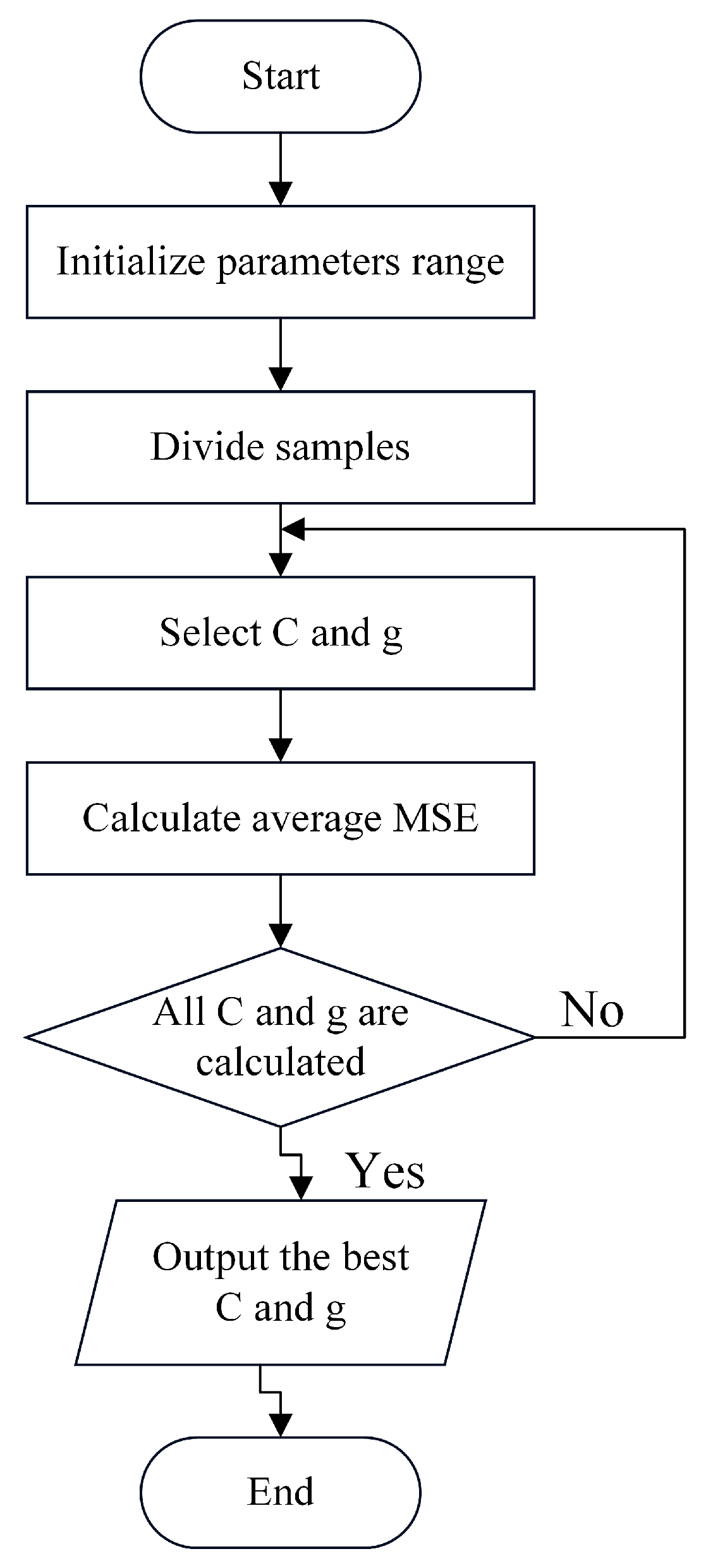
3.2. SVM Model for Diagnosis of ITSC Fault

The apFFT time-shift phase difference spectrum correction algorithm is used to calculate the fundamental frequency of the ZSVC, the fundamental component amplitudes of the traction motor’s ZSVC, and the three-phase current. The SVM-based fault diagnosis model of ITSC fault is established with the five parameters as input. The traction motor ITSC condition is classified as a normal condition, incipient fault condition, and serious fault condition using the proposed index. SVM is a machine learning method based on statistical theory, mainly used to solve classification and regression problems [49,50,51,52]. Its core idea is to complete the model training based on the structural risk minimization principle. It has nonlinear solid approximation ability, good generalization performance, and good results in dealing with small samples and nonlinear problems. SVM uses nonlinear mapping $\varphi (x)$ to map the original data to the high-dimensional space to deal with nonlinear regression problems of multidimensional data.

The C-SVC model is a relatively standard two-class SVM model. The train set is

$$T=\left\{\left(x_1,y_1\right),\cdots ,\left(x_l,y_l\right)\right\}\in {(X\times Y)}^l,$$

(13)

where $x_i\in X=R^n,y_i\in Y=\{1,-1\}(i=1,2,\cdots ,l)$, and x_i is the features vector.

Select kernel function $K\left(x,x^{\prime }\right)$ and appropriate parameter C. The standard kernel functions $K\left(x,x^{\prime }\right)$ mainly include linear, polynomial, and radial basis kernel functions. The Lagrange dual problem of the original problem is

$$\underset{\alpha }{\min }\frac{1}{2}{\displaystyle \sum _{i=1}^j{\displaystyle \sum _{j=1}^l{y}_i}}{y}_j{\alpha }_i{\alpha }_{j}K\left(x_i,x_j\right)-{\displaystyle \sum _{j=1}^l{\alpha }_j},$$

(14)

$$s.t.\hspace{1em}{\displaystyle \sum _{i=1}^l{y}_i}{\alpha }_i=0,\hspace{1em}0⩽{\alpha }_i⩽C,i=1,\cdots ,l$$

Obtain the optimal solution: ${\alpha }^{\ast }={\left({\alpha }_1^{\ast },\cdots ,{\alpha }_l^{\ast }\right)}^{\mathrm{T}}$.

Select a positive component of $0<{\alpha }_j^{\ast }<C$ from ${\alpha }^{\ast }$, and calculate the threshold accordingly:

$$b^{\ast }=y_j-{\displaystyle \sum _{i=1}^l{y}_i}{\alpha }_i^{\ast }K\left(x_i-x_j\right),$$

(15)

The constructed decision function is

$$f(x)=\mathrm{sgn}\left({\displaystyle \sum _{i=1}^l{\alpha }_i^{\ast }}{y}_{i}K\left(x,x_i\right)+b^{\ast }\right),$$

(16)

If the Gaussian radial basis function is used as the kernel function, g is the parameter of the Gaussian radial basis function:

$$K\left(x_i,x\right)=\exp \left(-\frac{{‖x_i-x_j‖}^2}{2\sigma }\right)=\exp \left(-g{‖x_i-x_j‖}^2\right).$$

(17)

In the SVM classification model, the selection of the model penalty parameter C and Gaussian kernel function parameter g is directly related to the model performance. The K-CV (K-fold cross-validation) is a standard cross-validation algorithm that divides datasets into K sub-datasets evenly in model training. Each sub-dataset is used as the validation set in turn, and the remaining K − 1 sub-datasets are used as the training set to train K models. The average mean square error (MSE) of K models on the validation set is used as the performance index. The mean square error is

$${\delta }_{\mathrm{MSE}}=\frac{1}{n}{\displaystyle \sum _{i=1}^n{(y_i-{\overline{y}}_i)}^2}.$$

(18)

In Formula (18), n is the number of samples, $y_i$ is the predicted value, and ${\overline{y}}_i$ is the target value.

Grid search is used to select several discrete points on each dimension of the parameter space according to certain rules. The discrete points of different dimensions intersect in the parameter space to obtain the discrete solution. Calculate each discrete solution to obtain the optimal solution. Figure 4 is the flow chart of the hyper-parameter optimization using K-CV and the grid search method. Take the grid point as C = 2^a, g = 2^b, and initialize the range of a and b, which are positive and negative integers. Parameters a and b are selected from the minimum to the maximum using 1 step of their range. K-CV is used to calculate the average MSE of the K models on the K validation sets. After calculating all the combinations of C and g at all grid intersections, C and g at the minimum average MSE are the optimal solutions.

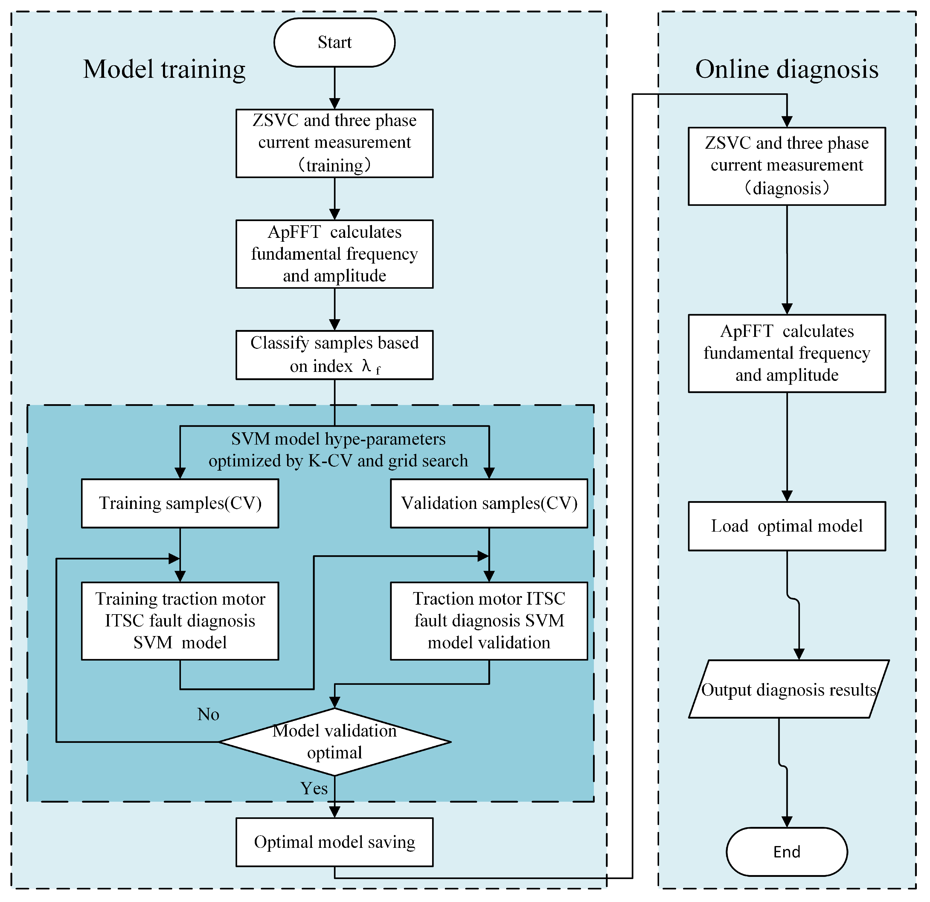
3.3. ITSC Fault Diagnosis Procedure Based on SVM Model

As shown in Figure 5, the EMU traction motor ITSC fault diagnosis based on SVM includes two stages: model training and online diagnosis. In the model training stage, the ZSVC and three-phase current are first measured with the circuit proposed in the article. Second, the apFFT time-shift phase difference correction algorithm is used to calculate the ZSVC fundamental frequency, the fundamental amplitudes of ZSVC, and the three-phase current. Third, the ZSVC fundamental frequency, the amplitude of ZSVC, and the three-phase current are used as features. Based on the ITSC fault index λ_f, the samples are divided into three categories: normal, incipient, and serious faults. Fourth, the K-CV method divides all the samples into training and validation samples. K-CV and the grid search method are used to optimize the hyper-parameters. Last, the optimal ITSC fault diagnosis model is saved. In the online diagnosis stage, the ITSC fault features are acquired similarly to the training stage. The optimal ITSC fault diagnosis model is loaded, and the fault features are input into the SVM model to predict the ITSC category.

4. EMU Electric Traction Simulation Experimental Platform

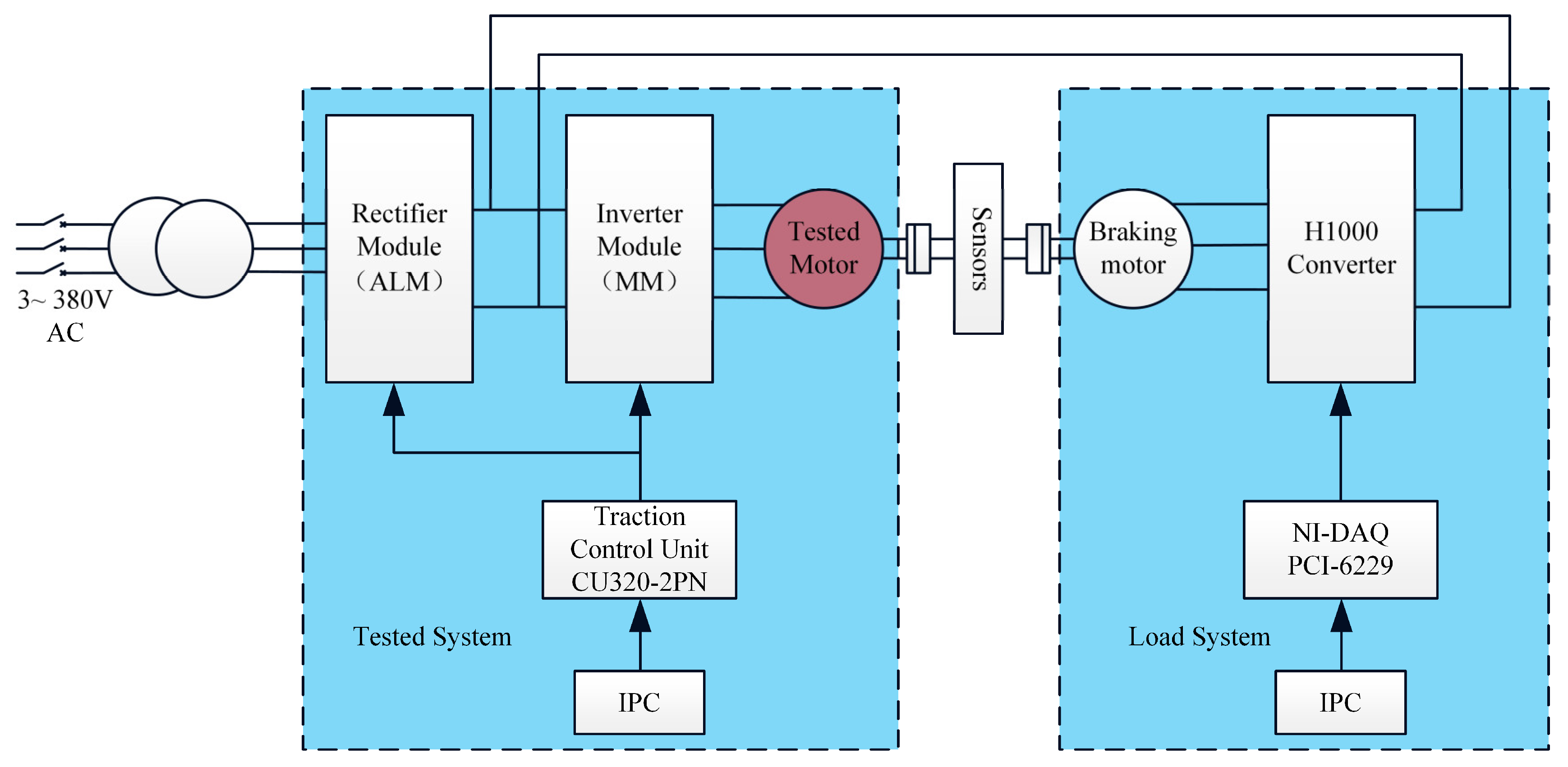
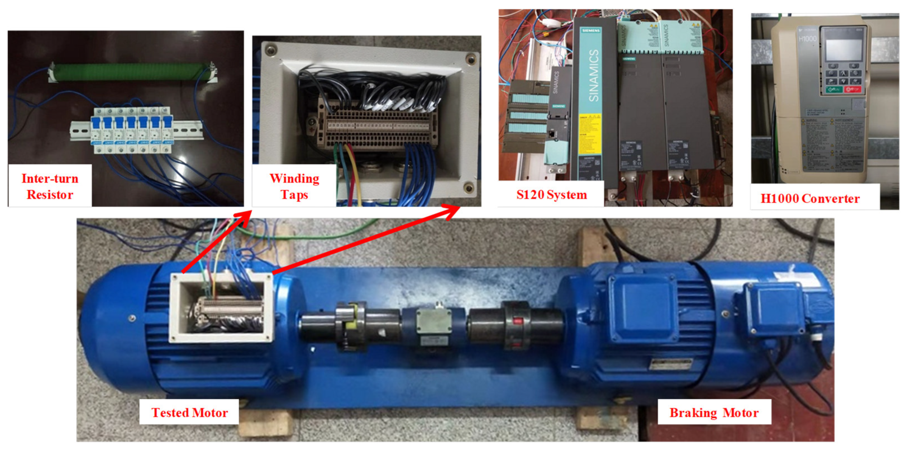
4.1. Overall Design of the Experimental Platform

The experimental data are acquired from the mutual-feed electric traction simulation experimental platform shown in Figure 6. The platform mainly includes the tested system and the load system. The tested system mainly includes an S120 variable frequency speed control system and the tested motor. The S120 controls the tested motor to operate according to the experimental conditions. The S120 system mainly includes the CU320-2PN control unit, ALM rectifier, and MM inverter modules. The load system mainly includes the braking motor and the H1000 converter. The PCI-6229 NI-DAQ gives the H1000 converter work instructions. The DC power supply of the tested system is obtained from the DC link of the load system. When the tested motor works in the motor state, the braking motor works in the generator state. The load system feeds electric energy back to the DC link to realize DC energy mutual feedback.

Figure 7 shows the main parts of the experimental platform. The tested motor is a three-phase AC asynchronous squirrel-cage motor with three-phase winding taps pulled out, whose parameters are shown in

Table 1. Rated parameters of the tested motor.

Parameter	Value	Parameter	Value
Power	5.5 kW	Frequency	50 Hz
Voltage	380 V	Speed	1445 rpm
Current	11.7 A	Turns per phase	162
Poles	4	Connection mode	Y
Magnetizing inductance	205.2 mH	Stator resistance	1.061 Ω
Rotor resistance	0.6269 Ω	Stator leakage inductance	3.217 mH
Rotor leakage inductance	7.349 mH	Inertia	0.1367 kg·m2

. The braking motor is a normal motor with the same type and power.

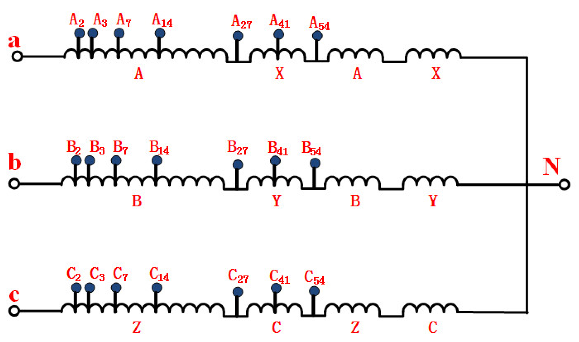
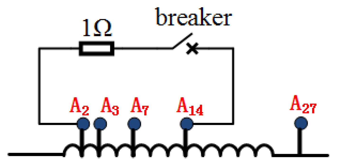
4.2. Setting ITSC Faults on Tested Motor

Figure 8 shows that the winding taps are pulled out at different stator winding turns during manufacturing to simulate the ITSC fault. The taps can be connected externally to simulate the short-circuit fault between different turns. The power resistor simulates the inter-turn resistor between non-metallic short-circuit turns. The vacuum breaker conveniently controls the short circuit of different turns loop.

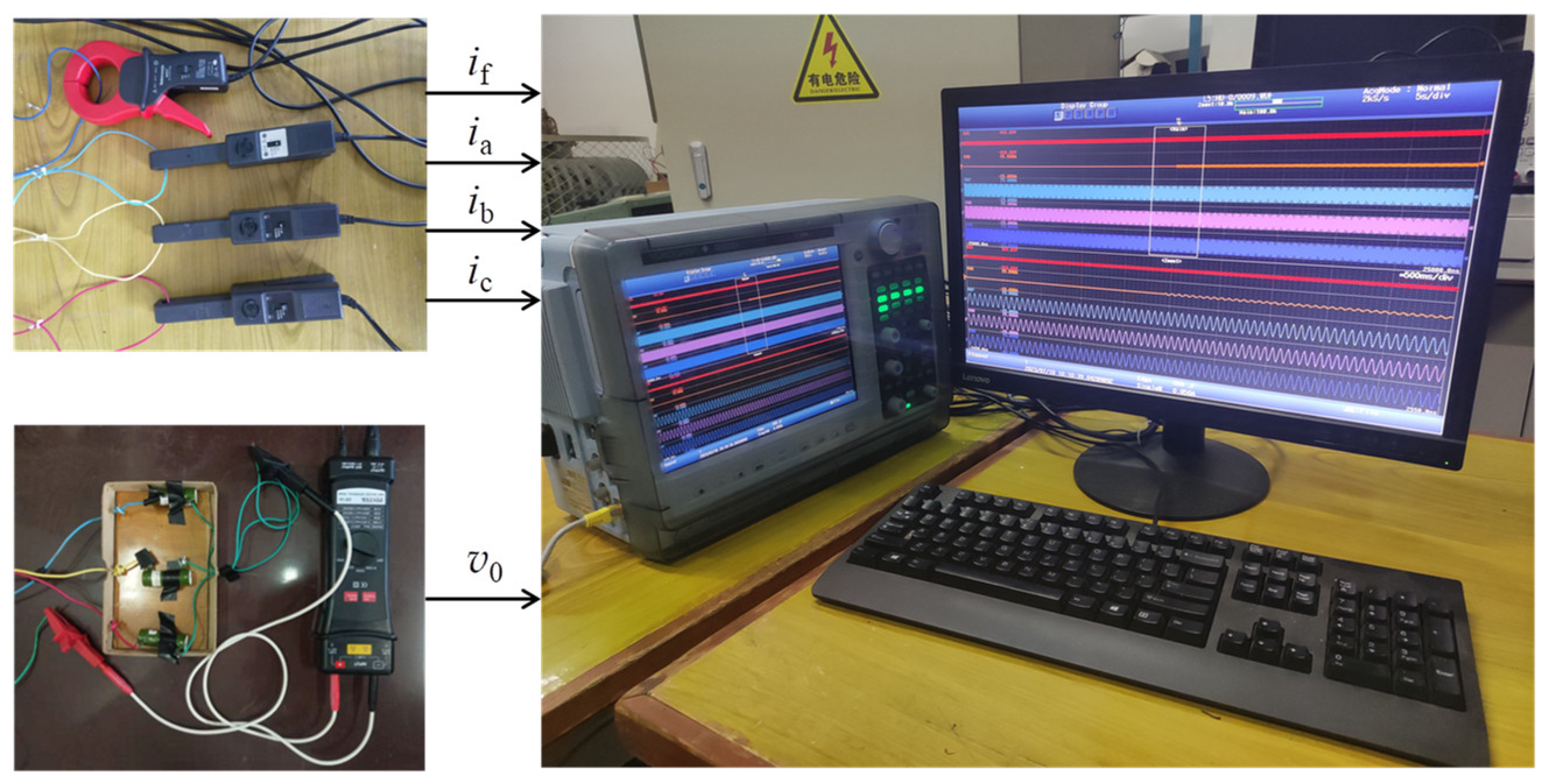
4.3. Signal Measurement of the Experimental Platform

The signal measurement is shown in Figure 9. The DL850E ScopeCorder produced by Yokogawa corporation in Japan is used for signal measurement whose LPF (low pass filter) is set to 400 Hz, and the sampling frequency is 2000 Hz. The A621 passive current probe is used to collect the inter-turn current, which cannot be measured in the actual application. If the inter-turn current is too large, it generates heat quickly to burn the motor. E3N active current probe is used to measure the three-phase current of the tested motor. The DP-50 voltage probe is used to measure the ZSVC using the measurement circuit shown in Figure 2. The ZSVC measurement balanced resistors are three 15 kΩ (1 kW) power resistors.

5. Analysis of ITSC Fault Diagnosis Model Based on Experimental Samples

During the experiment, the S120 converter system controlled the tested motor to operate in the torque control mode outputting a fixed electromagnetic torque. The H1000 converter controlled the braking motor according to the speed control mode running at a fixed speed. This experimental operation mode could simulate the steady operation conditions of EMU traction or electric braking at different speeds and torques.

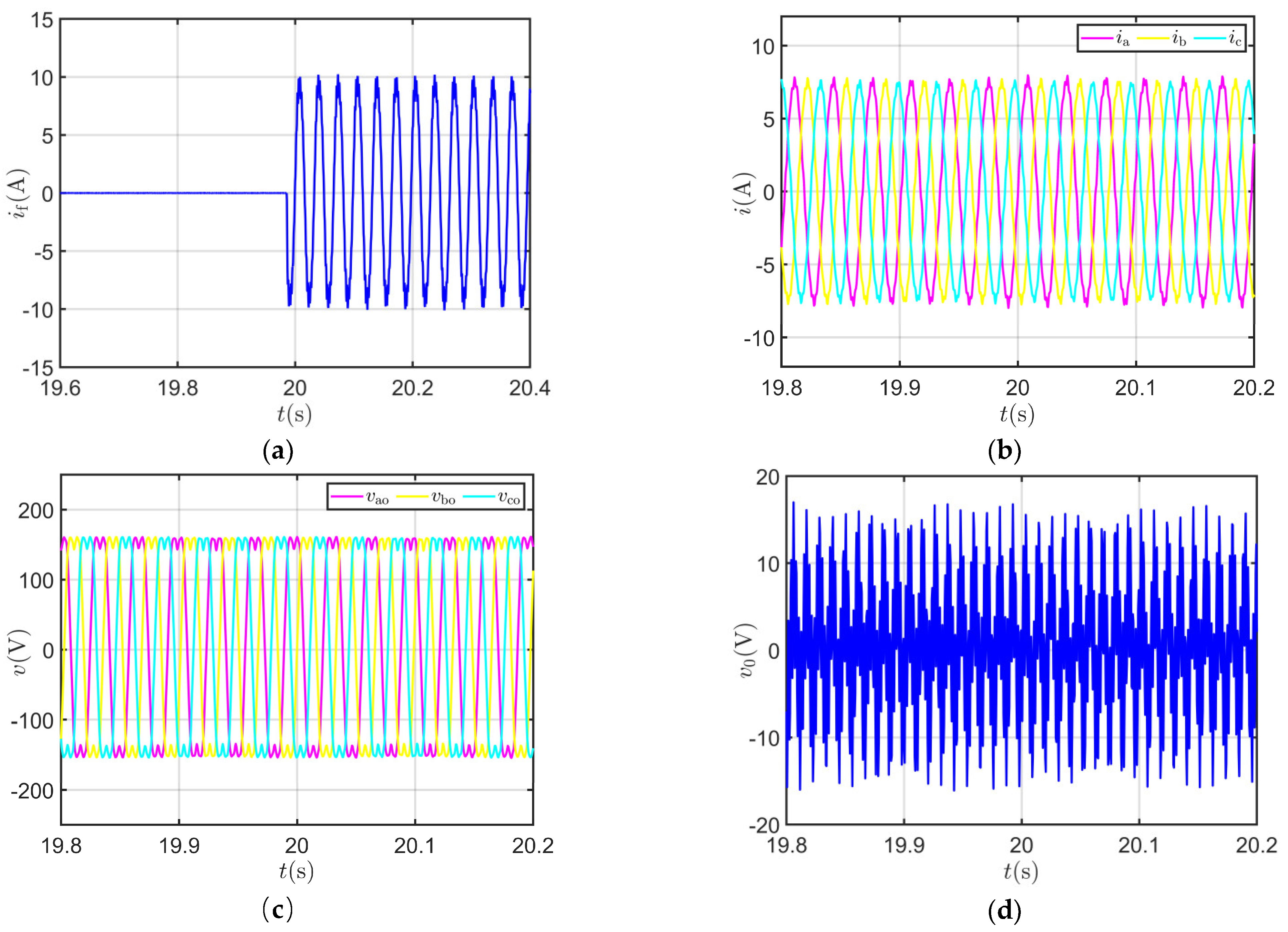
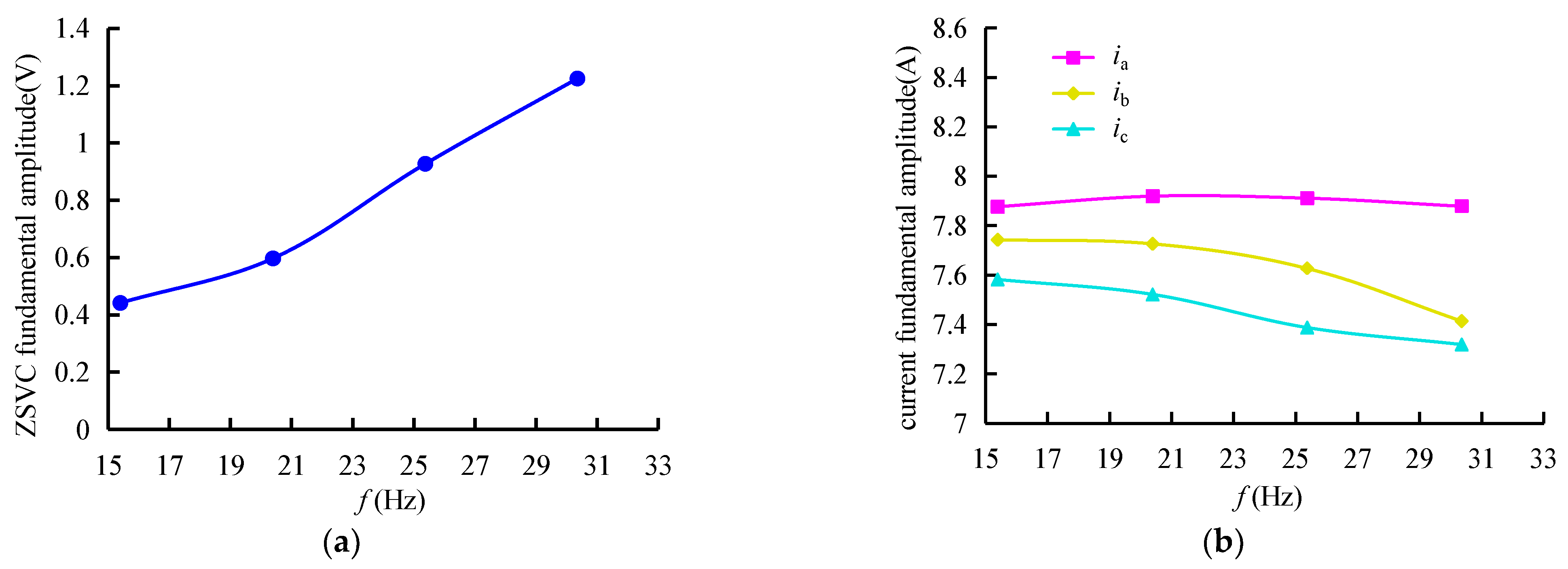
5.1. Analysis of Motor Signals with ITSC Fault

The tested fault motor ran at 900 rpm rotating speed with 10 Nm electromagnetic torque, 12 short-circuit turns ITSC fault in the a-phase stator winding, and a 1 Ω inter-turn resistor, as shown in Figure 10.

The insulation fault occurred at around 20 s. It can be seen from Figure 11a that when the stator winding ITSC fault occurs, a sinusoidal inter-turn current with the same fundamental frequency as the power supply is generated between the short-circuit turns. Figure 11b shows the three-phase current before and after the ITSC fault. Although the amplitude of the short-circuit current reached about 10 A, it had little impact on the three-phase current. Figure 11c shows the S120 system outputting three-phase voltage filtered by the 400 Hz LPF filter, and the outputting waveform conforms to the saddle waveform of SVPWM. Figure 11d shows the ZSVC before and after the ITSC fault, and the ZSVC will be studied and analyzed later.

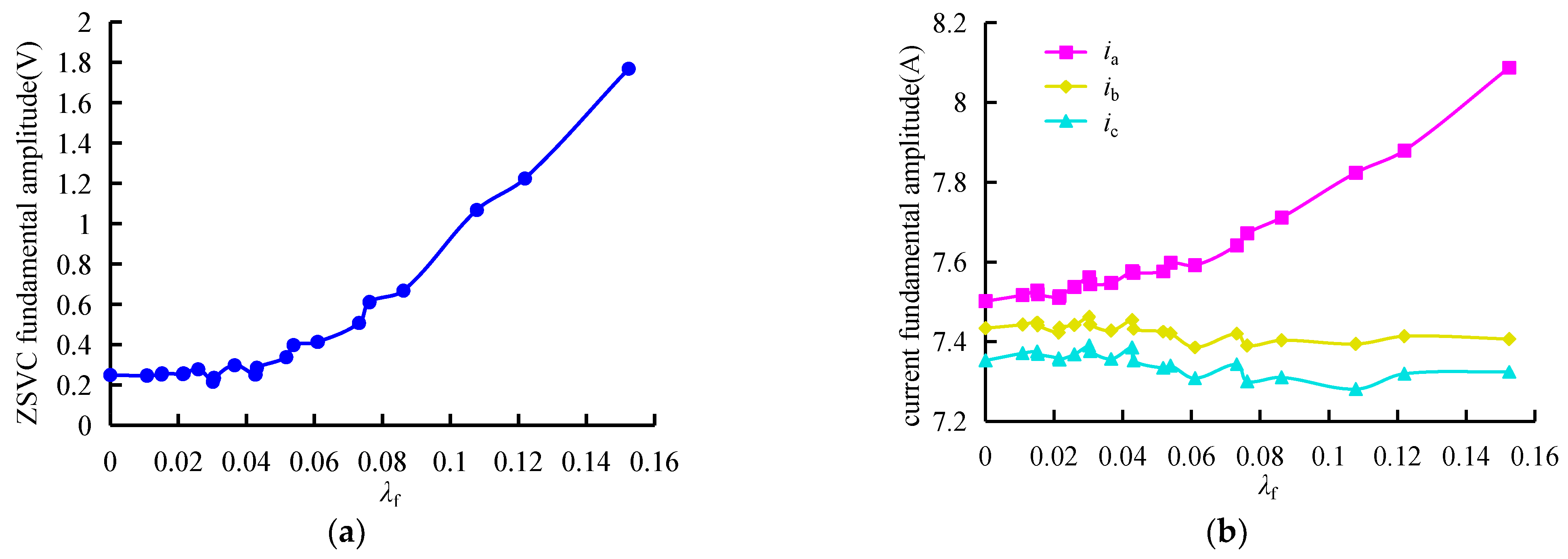
5.2. Analysis of ITSC Fault Features

The tested motor setting speed was 900 rpm, and the electromagnetic torque was set to 10 Nm. There was an ITSC fault in the a-phase winding. The frequency of the ZSVC fundamental component, the fundamental amplitudes of ZSVC, and the three-phase current were calculated using the apFFT time-shift spectrum correction algorithm with double Hanning windows. Based on Formula (12), 20 different indexes λ_f were calculated according to 5 different numbers of short-circuit turns and 4 different inter-turn resistances, as shown in

Table 2. The ITSC fault set and the extent index λ_f.

	Turns	5	7	12	20	25
Resistance (Ω)
1		0.03049	0.04268	0.07317	0.12195	0.15244
2		0.02156	0.03018	0.05174	0.08623	0.10779
4		0.01524	0.02134	0.03659	0.06098	0.07622
8		0.01078	0.01509	0.02587	0.04312	0.05390

.

It can be seen from Figure 12a that the ZSVC fundamental amplitude of the tested motor increased with the fault extent index λ_f. The fundamental amplitude of the ZSVC was about 0.2 V under normal conditions, mainly caused by the asymmetry of the three-phase winding. It can be seen from Figure 12b that the fundamental amplitude of the a-phase current increased with the ITSC fault extent. The b-phase and c-phase currents changed little. Similarly, because of the unbalance of the three-phase winding, the three-phase current was unbalanced under normal conditions.

The electromagnetic torque was set to 10 Nm, and the ITSC fault extent index λ_f was 0.07317. It can be seen from Figure 13a that in the process speed regulation, the fundamental frequency changed with the experimental system setting speed. According to the control characteristics of variable frequency speed regulation, the three-phase voltage increased linearly with the increase in speed. The ZSVC also increased with the tested motor’s fundamental frequency under the same λ_f. Figure 13b shows that the a-phase current did not change much, but the b-phase and c-phase currents decreased significantly with the increase of the fundamental frequency. The asymmetry of the three-phase current became more and more prominent.

According to the analysis above, the ZSVC fundamental component amplitude and the three-phase current asymmetry increases with the ITSC fault extent under fixed electromagnetic torque and speed. The three-phase current amplitude can reflect the electromagnetic torque value, and the speed is approximately linear with the fundamental frequency. Therefore, the ZSVC fundamental frequency, the fundamental amplitudes of ZSVC, and the three-phase current are selected as the features to establish the ITSC fault diagnosis model.

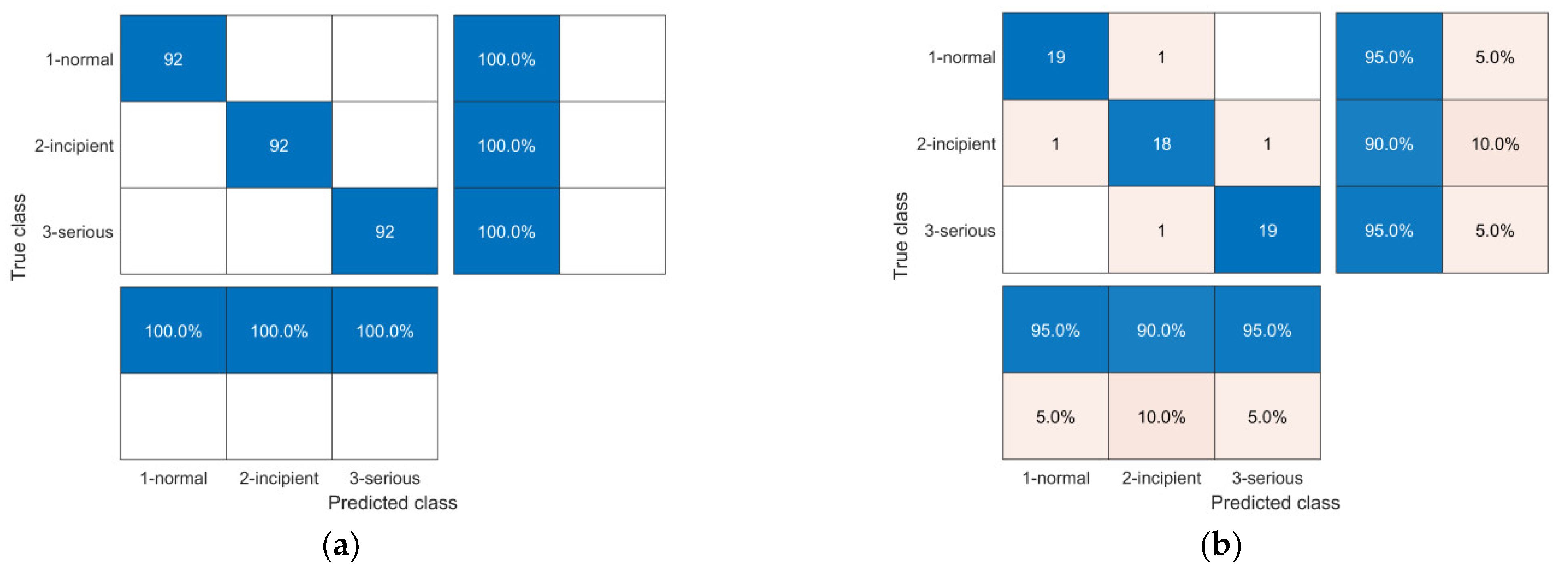
5.3. Analysis of SVM ITSC Fault Diagnosis Model Performance

The tested motor’s data acquisition conditions are shown in

Table 3. The working condition and the ITSC fault setting.

Speed (rpm)	Torque (Nm)	Turns	Resistance (Ω)
450, 600, 750, 900	2, 10, 18, 26	5, 7, 12, 20, 25	1, 2, 4, 8

. The tested motor with each fault extent index operated under four different speeds and electromagnetic torques. There were 16 working conditions in which the speeds or electromagnetic torques were different, and 7 normal samples needed to be acquired at each working condition to first obtain a total of 112 normal samples. There were 20 different ITSC fault extent λ_f samples under each speed and electromagnetic torque, as shown in Table 2. The classification of fault severity categories is determined by the application situation defined by users. In the experiment, the samples with 0.03018 ≤ λ_f < 0.06098 were defined as incipient ITSC fault samples because the thermal power caused by inter-turn short-circuit fault was small. Samples with 0.06098 ≤ λ_f were considered serious ITSC fault samples because the thermal power was large. Thus the ITSC fault samples were divided into 112 incipient and 112 serious ITSC fault samples. The SVM-based ITSC fault diagnosis model was established by selecting 92 samples from each category as train samples and 20 samples from each category as the test samples. The grid search range was a = [−5, 5], b = [−5, 5]. The parameter K was 3 in the K-CV method.

Figure 14 shows the prediction results of the SVM-based ITSC fault diagnosis model on the experimental samples. Figure 14a shows that there is no misclassification on the training dataset. Figure 14a shows that there is a sample misclassified among the normal and incipient samples and a sample misclassified among incipient and serious samples. There is no misclassification between the normal and the serious fault samples. The model’s prediction accuracy is 100% on the training dataset and 93.33% on the test dataset, which indicates that the model can detect and evaluate the ITSC fault accurately.

6. Conclusions

The ITSC fault diagnosis of the asynchronous traction motor significantly ensures the EMU’s safe operation and saves maintenance costs. The non-metallic ITSC fault extent evaluating index λ_f was proposed based on the short-circuit thermal power. The index λ_f is related to the number of short-circuit turns and inter-turn resistance. The apFFT time-shift phase difference spectrum correction with double Hanning windows was used to calculate five parameters used as fault features to train SVM model to diagnose the ITSC fault, and the SVM model hyper-parameters C and g were optimized using K-CV and the grid search method. The method proposed in the article can detect and evaluate the ITSC fault of traction motors in a speed control system under vector control or direct torque control conditions in which the fundamental frequency of supply voltage is unknown. EMU traction motors work at different speeds and torque points during operation. The prediction results of different steady-state operating points can be integrated to improve the accuracy of the fault diagnosis model. The method can be used when the traction motor is in a steady state, and it cannot be used if the traction motor accelerates or decelerates.

References

1. Lee, S.-G. A Study on Traction Motor Characteristic in EMU Train. In Proceedings of the 13th International Conference on Control, Automation and Systems, Gyeonggi-do, Republic of Korea, 22–25 October 2014. [Google Scholar]
2. Zhang, K.; Jiang, B.; Chen, F. Multiple-Model-Based Diagnosis of Multiple Faults With High-Speed Train Applications Using Second-Level Adaptation. IEEE Trans. Ind. Electron. 2021, 68, 6257–6266. [Google Scholar] [CrossRef]
3. Chen, Z.P.; Wang, Z.; Jia, L.M.; Cai, G.Q. Analysis and Comparison of Locomotive Traction Motor Intelligent Fault Diagnosis Methods. Appl. Mech. Mater. 2011, 97–98, 994–1002. [Google Scholar] [CrossRef]
4. Al-Ameri, S.M.; Alawady, A.A.; Yousof, M.F.M.; Kamarudin, M.S.; Salem, A.A.; Abu-Siada, A.; Mosaad, M.I. Application of Frequency Response Analysis Method to Detect Short-Circuit Faults in Three-Phase Induction Motors. Appl. Sci. 2022, 12, 2046. [Google Scholar] [CrossRef]
5. Chao, C.; Wang, W.; Chen, H.; Zhang, B.; Shao, J.; Teng, W. Enhanced Fault Diagnosis Using Broad Learning for Traction Systems in High-Speed Trains. IEEE Trans. Power Electron. 2020, 36, 7461–7469. [Google Scholar] [CrossRef]
6. Guo, X.; Tang, Y.; Wu, M.; Zhang, Z.; Yuan, J. FPGA-Based Hardware-in-the-Loop Real-Time Simulation Implementation for High-Speed Train Electrical Traction System. IET Electr. Power Appl. 2020, 14, 850–858. [Google Scholar] [CrossRef]
7. Kaufhold, M.; Aninger, H. Electrical Stress and Failure Mechanism of the Winding Insulation in PWM-Inverter-Fed Low-Voltage Induction Motors. IEEE Trans. Ind. Electron. 2000, 2, 396–402. [Google Scholar] [CrossRef]
8. Mbaye, A.; Bellomo, J.P. Electrical Stresses Applied to Stator Insulation in Low-Voltage Induction Motors Fed by PWM Drives. IET Electr. Power Appl. 1997, 144, 191–198. [Google Scholar] [CrossRef]
9. Hwang, D.H.; Park, D.Y.; Kim, Y.J.; Lee, Y.H.; Hur, I.G. A Comparison with Insulation System for PWM-Inverter-Fed Induction Motors. In Proceedings of the International Conference on Electrical Machines & Systems, Shenyang, China, 18–20 August 2001. [Google Scholar] [CrossRef]
10. Otero, M.; Barrera, P.; Bossio, G.R.; Leidhold, R. Stator Inter-turn Faults Diagnosis in Induction Motors Using Zero-sequence Signal Injection. IET Electr. Power Appl. 2020, 14, 273–2738. [Google Scholar] [CrossRef]
11. Singh, M.; Shaik, A.G. Incipient Fault Detection in Stator Windings of an Induction Motor Using Stockwell Transform and SVM. IEEE Trans. Instrum. Meas. 2020, 69, 9496–9504. [Google Scholar] [CrossRef]
12. Sonje, D.M.; Kundu, P.; Chowdhury, A. A Novel Approach for Sensitive Inter-turn Fault Detection in Induction Motor Under Various Operating Conditions. Arab. J. Sci. Eng. 2019, 44, 6887–6900. [Google Scholar] [CrossRef]
13. Namdar, A. A robust principal component analysis-based approach for detection of a stator inter-turn fault in induction motors. Prot. Control. Mod. Power Syst. 2022, 7, 48. [Google Scholar] [CrossRef]
14. Mejia-Barron, A.; Tapia-Tinoco, G.; Razo-Hernandez, J.R.; Valtierra-Rodriguez, M.; Granados-Lieberman, D. A neural network-based model for MCSA of ITSC faults in induction motors and its power hardware in the loop simulation. Comput. Electr. Eng. 2021, 93, 107234. [Google Scholar] [CrossRef]
15. Tallam, R.; Habetler, T.; Harley, R. Transient model for induction machines with stator winding turn faults. IEEE Trans. Ind. Appl. 2002, 38, 632–637. [Google Scholar] [CrossRef]
16. Zhao, Z.; Fan, F.; Wang, W.; Liu, Y.; See, K.Y. Detection of Stator Interturn Short-Circuit Faults in Inverter-Fed Induction Motors by Online Common-Mode Impedance Monitoring. IEEE Trans. Instrum. Meas. 2021, 70, 3513110. [Google Scholar] [CrossRef]
17. Duan, F.; Zivanovic, R. Induction Motor Stator Fault Detection by a Condition Monitoring Scheme Based on Parameter Estimation Algorithms. Electr. Power Compon. Syst. 2016, 44, 1138–1148. [Google Scholar] [CrossRef] [Green Version]
18. Bazine, I.B.A.; Tnani, S.; Poinot, T.; Champenois, G.; Jelassi, K. On-Line Detection of Stator and Rotor Faults Occurring in In-duction Machine Diagnosis by Parameters Estimation. In Proceedings of the 8th IEEE Symposium on Diagnostics for Electrical Machines, Power Electronics & Drives, Bologna, Italy, 5–8 September 2011. [Google Scholar] [CrossRef]
19. Abdallah, H.; Benatman, K. Stator winding inter-turn short-circuit detection in induction motors by parameter identification. IET Electr. Power Appl. 2017, 11, 272–288. [Google Scholar] [CrossRef]
20. Nguyen, V.; Seshadrinath, J.; Wang, D.; Nadarajan, S.; Vaiyapuri, V. Model-Based Diagnosis and RUL Estimation of Induction Machines Under Interturn Fault. IEEE Trans. Ind. Appl. 2017, 53, 2690–2701. [Google Scholar] [CrossRef]
21. Kallesoe, C.S.; Vadstrup, P.; Rasmussen, H.; Izadi-Zamanabadi, R. Observer Based Estimation of Stator Winding Faults in Delta-Connected Induction Motors, a LMI Approach. In Proceedings of the IAS Annual Meeting, Tampa, FL, USA, 8–12 October 2006. [Google Scholar] [CrossRef]
22. De Angelo, C.H.; Bossio, G.R.; Giaccone, S.J.; Valla, M.I.; Solsona, J.A.; Garcia, G.O. Online Model-Based Stator-Fault Detection and Identification in Induction Motors. IEEE Trans. Ind. Electron. 2009, 56, 4671–4680. [Google Scholar] [CrossRef]
23. Guezmil, A.; Berriri, H.; Pusca, R.; Sakly, A.; Romary, R.; Mimouni, M.F. Detecting Inter-Turn Short-Circuit Fault in Induction Machine Using High-Order Sliding Mode Observer: Simulation and Experimental Verification. J. Control. Autom. Electr. Syst. 2017, 28, 532–540. [Google Scholar] [CrossRef]
24. Kia, M.Y.; Khedri, M.; Najafi, H.R.; Nejad, M.A.S. Hybrid modelling of doubly fed induction generators with inter-turn stator fault and its detection method using wavelet analysis. IET Gener. Transm. Distrib. 2013, 7, 982–990. [Google Scholar] [CrossRef]
25. Kumar, P.S.; Xie, L.; Halick, M.S.M.; Vaiyapuri, V. Stator End-Winding Thermal and Magnetic Sensor Arrays for Online Stator Inter-Turn Fault Detection. IEEE Sens. J. 2020, 21, 5312–5321. [Google Scholar] [CrossRef]
26. Chen, P.; Xie, Y.; Hu, S. Electromagnetic Performance and Diagnosis of Induction Motors With Stator Interturn Fault. IEEE Trans. Ind. Appl. 2020, 57, 1354–1364. [Google Scholar] [CrossRef]
27. Lee, S.-H.; Wang, Y.-Q.; Song, J.-I. Fourier and wavelet transformations application to fault detection of induction motor with stator current. J. Cent. S. Univ. Technol. 2010, 17, 93–101. [Google Scholar] [CrossRef]
28. Liu, H.; Huang, J.; Hou, Z.; Yang, J.; Ye, M. Stator inter-turn fault detection in closed-loop controlled drive based on switching sideband harmonics in CMV. IET Electr. Power Appl. 2017, 11, 178–186. [Google Scholar] [CrossRef]
29. Sadeghi, R.; Samet, H.; Ghanbari, T. Detection of Stator Short-Circuit Faults in Induction Motors Using the Concept of Instantaneous Frequency. IEEE Trans. Ind. Inform. 2018, 15, 4506–4515. [Google Scholar] [CrossRef]
30. Vinayak, B.A.; Anand, K.A.; Jagadanand, G. Wavelet-based real-time stator fault detection of inverter-fed induction motor. IET Electr. Power Appl. 2019, 14, 82–90. [Google Scholar] [CrossRef]
31. Almounajjed, A.; Sahoo, A.K.; Kumar, M.K. Diagnosis of stator fault severity in induction motor based on discrete wavelet analysis. Measurement 2021, 182, 109780. [Google Scholar] [CrossRef]
32. Tian, R.; Chen, F.; Dong, S. Compound Fault Diagnosis of Stator Interturn Short Circuit and Air Gap Eccentricity Based on Random Forest and XGBoost. Math. Probl. Eng. 2021, 42, 2149048. [Google Scholar] [CrossRef]
33. Xu, Z.; Hu, C.; Yang, F.; Kuo, S.-H.; Goh, C.-K.; Gupta, A.; Nadarajan, S. Data-Driven Inter-Turn Short Circuit Fault Detection in Induction Machines. IEEE Access 2017, 5, 25055–25068. [Google Scholar] [CrossRef]
34. Husari, F.; Seshadrinath, J. Incipient Interturn Fault Detection and Severity Evaluation in Electric Drive System Using Hybrid HCNN-SVM Based Model. IEEE Trans. Ind. Inform. 2021, 18, 1823–1832. [Google Scholar] [CrossRef]
35. Rajamany, G.; Srinivasan, S.; Rajamany, K.; Natarajan, R.K. Induction Motor Stator Interturn Short Circuit Fault Detection in Accordance with Line Current Sequence Components Using Artificial Neural Network. J. Electr. Comput. Eng. 2019, 1, 4825787. [Google Scholar] [CrossRef]
36. Bensaoucha, S.; Ameur, A.; Bessedik, S.A.; Moati, Y. Artificial Neural Networks Technique to Detect and Locate an Interturn Short-Circuit Fault in Induction Motor. In Renewable Energy for Smart and Sustainable Cities; Hatti, M., Ed.; Lecture Notes in Networks and Systems; Springer International Publishing: Cham, Switzerland, 2019; Volume 62, pp. 103–113. ISBN 978-3-030-04788-7. [Google Scholar]
37. Skowron, M.; Orlowska-Kowalska, T.; Wolkiewicz, M.; Kowalski, C.T. Convolutional Neural Network-Based Stator Current Data-Driven Incipient Stator Fault Diagnosis of Inverter-Fed Induction Motor. Energies 2020, 13, 1475. [Google Scholar] [CrossRef] [Green Version]
38. Urresty, J.-C.; Riba, J.-R.; Romeral, L. Application of the ZSVC component to detect stator winding inter-turn faults in PMSMs. Electr. Power Syst. Res. 2012, 89, 38–44. [Google Scholar] [CrossRef]
39. Hang, J.; Zhang, J.; Cheng, M.; Huang, J. Online Interturn Fault Diagnosis of Permanent Magnet Synchronous Machine Using Zero-Sequence Components. IEEE Trans. Power Electron. 2015, 30, 6731–6741. [Google Scholar] [CrossRef]
40. Cash, M.; Habetler, T.; Kliman, G. Insulation failure prediction in AC machines using line-neutral voltages. IEEE Trans. Ind. Appl. 1998, 34, 1234–1239. [Google Scholar] [CrossRef]
41. Cash, M.A.; Habetler, T.G. Insulation failure prediction in inverter-fed induction machines using line-neutral voltages. In Proceedings of the IAS Annual Meeting, New Orleans, LA, USA, 5–9 October 1997. [Google Scholar] [CrossRef]
42. Garcia, P.; Briz, F.; Degner, M.W.; Diez, A.B. Diagnostics of Induction Machines Using the Zero Sequence Voltage. In Proceedings of the IAS Annual Meeting, Seattle, WA, USA, 3–7 October 2004. [Google Scholar] [CrossRef]
43. Wang, Z.H.; Huang, X.D. Principle of Phase Measurement and Its Application Based on All-Phase Spectral Analysis. J. Data Acquis Process 2009, 24, 777–782. [Google Scholar] [CrossRef]
44. Huang, X.D.; Wang, Z.H. Anti-noise Performance of All-phase FFT Phase Measuring Method. J. Data Acquis Process 2011, 26, 286–291. [Google Scholar] [CrossRef]
45. Huang, K.H.; Wang, D.M.; Zhu, Z.Y.; Wei, H.F.; Jiang, W.U. Power System Harmonic Detection Algorithm Based on Co-sin-Window and Interpolated FFT and APFFT. Comput. Technol. Dev. 2011, 21, 223–230. [Google Scholar]
46. Huang, X.; Wang, Y.; Jin, X.; Lü, W. No-Windowed ApFFT/FFT Phase Difference Frequency Estimator Based on Frequency-Shift & Compensation. J. Electron. Inf. 2016, 38, 124–131. [Google Scholar] [CrossRef]
47. Qi, G.Q.; Jia, X.L. High-Accuray Frequency and Phase Estimation of single-Tone Based on Phase of DFT. Acta Electron. Sin. 2001, 9, 1164–1167. [Google Scholar] [CrossRef]
48. Li, X.F.; Li, L.; Kou, K.; Wu, T.F.; Yang, Y. Analysis and Improvement of Time-Shift Phase Difference Spectral Correction Based on All-Phase FFT. J. Tianjin Univ. Sci. Technol. 2016, 49, 1290–1295. [Google Scholar]
49. Li, S. Multi-Sensor Fusion by CWT-PARAFAC-IPSO-SVM for Intelligent Mechanical Fault Diagnosis. Sensors 2022, 22, 367. [Google Scholar] [CrossRef]
50. Todkar, S.S.; Baltazart, V.; Ihamouten, A.; Dérobert, X.; Guilbert, D. One-class SVM based outlier detection strategy to detect thin interlayer debondings within pavement structures using Ground Penetrating Radar data. J. Appl. Geophys. 2021, 192, 104392. [Google Scholar] [CrossRef]
51. Guan, S.; Wang, X.; Hua, L.; Li, L. Quantitative ultrasonic testing for near-surface defects of large ring forgings using feature extraction and GA-SVM. Appl. Acoust. 2020, 173, 107714. [Google Scholar] [CrossRef]
52. Zhao, Y.; Wei, G. Using an Improved PSO-SVM Model to Recognize and Classify the Image Signals. Complexity 2021, 21, 8328532. [Google Scholar] [CrossRef]
Figure 1. ZSVC measurement circuit.
Energies 16 05612 g001
Figure 2. N-order apFFT calculation method.
Energies 16 05612 g002
Figure 3. Data truncation for time-shift phase difference correction.
Energies 16 05612 g003
Figure 4. Flow chart of the hyper-parameters optimization.
Energies 16 05612 g004
Figure 5. Procedure of the ITSC fault diagnosis based on SVM model.
Energies 16 05612 g005
Figure 6. Energy mutual-feed electric traction simulation experimental platform.
Energies 16 05612 g006
Figure 7. Main parts of the EMU electric traction simulation experimental platform.
Energies 16 05612 g007
Figure 8. Stator winding taps pulled out of the tested motor.
Energies 16 05612 g008
Figure 9. Signal measurements of the tested motor.
Energies 16 05612 g009
Figure 10. The stator ITSC fault set on the a-phase.
Energies 16 05612 g010
Figure 11. Signals of the tested system before and after ITSC fault: (a) inter-turn current of the tested motor; (b) three-phase current of the tested motor; (c) three-phase voltage of S120 inverter module; (d) ZSVC of the tested motor.
Energies 16 05612 g011
Figure 12. Influence of ITSC fault on the tested motor signal fundamental amplitude: (a) influence of ITSC fault on ZSVC fundamental amplitude; (b) influence of ITSC fault on three-phase current fundamental amplitude.
Energies 16 05612 g012
Figure 13. Influence of frequency on the tested motor signal fundamental amplitude: (a) influence of frequency on ZSVC fundamental amplitude; (b) influence of frequency on three-phase current fundamental amplitude.
Energies 16 05612 g013
Figure 14. Confusion matrix of ITSC fault diagnosis SVM model: (a) confusion matrix of SVM model on the training dataset; (b) confusion matrix of SVM model on the test dataset.
Energies 16 05612 g014