Article

Investigating Winter Temperatures in Sweden and Norway: Potential Relationships with Climatic Indices and Effects on Electrical Power and Energy Systems

by
Younes Mohammadi
1,*,
Aleksey Palstev
2,
Boštjan Polajžer
3,
Seyed Mahdi Miraftabzadeh
4 and
Davood Khodadad
1
1
Department of Applied Physics and Electronics, Umeå University, 90187 Umeå, Sweden
2
Department of Ecology and Environmental Science, Umeå University, 90187 Umeå, Sweden
3
Faculty of Electrical Engineering and Computer Science, University of Maribor, 2000 Maribor, Slovenia
4
Department of Energy, Politecnico di Milano, Via Lambruschini 4, 20156 Milano, Italy
*
Author to whom correspondence should be addressed.
Energies 2023, 16(14), 5575; https://doi.org/10.3390/en16145575
Submission received: 22 March 2023 / Revised: 10 July 2023 / Accepted: 22 July 2023 / Published: 24 July 2023
(This article belongs to the Special Issue Climate Changes and the Impacts on Power and Energy Systems)

Abstract

:
This paper presents a comprehensive study of winter temperatures in Norway and northern Sweden, covering a period of 50 to 70 years. The analysis utilizes Singular Spectrum Analysis (SSA) to investigate temperature trends at six selected locations. The results demonstrate an overall long-term rise in temperatures, which can be attributed to global warming. However, when investigating variations in highest, lowest, and average temperatures for December, January, and February, 50% of the cases exhibit a significant decrease in recent years, indicating colder winters, especially in December. The study also explores the variations in Atlantic Meridional Overturning Circulation (AMOC) variations as a crucial climate factor over the last 15 years, estimating a possible 20% decrease/slowdown within the first half of the 21st century. Subsequently, the study investigates potential similarities between winter AMOC and winter temperatures in the mid to high latitudes over the chosen locations. Additionally, the study examines another important climatic index, the North Atlantic Oscillation (NAO), and explores possible similarities between the winter NAO index and winter temperatures. The findings reveal a moderate observed lagged correlation for AMOC-smoothed temperatures, particularly in December, along the coastal areas of Norway. Conversely, a stronger lagged correlation is observed between the winter NAO index and temperatures in northwest Sweden and coastal areas of Norway. Thus, NAO may influence both AMOC and winter temperatures (NAO drives both AMOC and temperatures). Furthermore, the paper investigates the impact of colder winters, whether caused by AMOC, NAO, or other factors like winds or sea ice changes, on electrical power and energy systems, highlighting potential challenges such as reduced electricity generation, increased electricity consumption, and the vulnerability of power grids to winter storms. The study concludes by emphasizing the importance of enhancing the knowledge of electrical engineering researchers regarding important climate indices, AMOC and NAO, the possible associations between them and winter temperatures, and addressing the challenges posed by the likelihood of colder winters in power systems.

1. Introduction

1.1. Problem Description

Climate change has heightened global concerns, imposing a comprehensive understanding of its regional effects to develop effective adaptation strategies. In Scandinavia, Sweden and Norway face severe winters that rely heavily on stable electrical power and energy systems to meet specifically heightened heating demands. However, studies such as [1,2] indicate that climate change may induce substantial alterations in the Atlantic Meridional Overturning Circulation (AMOC), as a crucial component of global oceanic circulation. The AMOC includes a northward surface warm water flow (upper 1000 m) of North Atlantic drift, which is balanced by the southward cold deep flow (1000–5000 m) [2,3,4]. It plays an essential role in climate by transporting heat, freshwater, and carbon [5,6,7]. AMOC-associated poleward heat transport substantially contributes to the North American and continental European climates [8,9]. The Gulf Stream (GS), in contrast to other western boundary currents, is expected to slow down because of the AMOC weakening. North Atlantic Oscillation (NAO) is also another key climatic index. According to a traditional definition, it is “the difference of normalized sea level pressure anomaly between Iceland and the subtropical eastern North Atlantic” [10]. The changes in AMOC/GS, in terms of weakening, have the potential to impact winter temperatures in the European climate [11] and possibly the regions of Scandinavia. The impact of NAO on the AMOC and/or climate change is also probable [12,13]. Consequently, investigating the possible influence of AMOC/NAO on Sweden and Norway’s winter temperatures becomes imperative to assess the vulnerability of their power and energy systems. Hence, there is a knowledge gap in analyzing historical temperature data, examining AMOC/NAO variations, and evaluating their potential effects on power generation and energy systems.

1.2. Literature Review

Several studies have been conducted on the AMOC and GS patterns and trends. The variability in the AMOC is credited to wind forcing (interannual time) and to geostrophic forces (interannual to decadal scales) [14]. Increased freshwater fluxes from melting Arctic Sea and land ice can make “open-ocean convection” and “deep-water formation” weaker in the Labrador and Irminger Seas, leading to AMOC weakening [11,15]. While one study [15] has suggested that the AMOC has weakened over the past 13,000 years, and another study [16] suggested slowing on faster timescales, there is insufficient data-based evidence to support a conclusion of AMOC-weakening strength over the 20th century in a long-term view [17] or the last 50 years [14]. Some studies have shown long-term trends [18,19]; however, combining sparse data and large cyclic variability may also cause an improper understanding [20]. Later, several high-resolution modeling studies, constrained with limited data, suggested that the detected AMOC weakening at 26° N from 2004 is mainly due to natural variability and that anthropogenic forcing has not yet produced a substantial AMOC weakening. In addition, direct observations of the AMOC in the South Atlantic fail to demonstrate an anthropogenic trend unambiguously. Moreover, under a higher scenario (RCP (Representative Concentration Pathway) 8.5) in CMIP5 (Coupled Model Intercomparison Project Phase 5) simulations, the AMOC will likely weaken over the 21st century [21], with a decline ranging from 12 to 54% (with uncertainty in the AMOC behavior projections). Another study [22] predicts a possible AMOC decline between 34 and 45% over the 21st century. According to this study, in a lower scenario, such as RCP4.5, CMIP5 models forecast a 20% AMOC weakening within the first half of the 21st century, followed by a subsequent stabilization (minor recovery). The projected AMOC weakening will be counteracted by deep ocean warming (below 700 m), which will be disposed to make the AMOC strong. The saltiness transport versus observations in the models, as a criterion of AMOC stability, showed complicated situations.
However, some argue that coupled climate models require correction for the known bias and that AMOC variations could be even larger than the gradual decreases predicted by most models, explaining if the AMOC were to entirely shut down and “flip states”. Any AMOC slowdown could result in less heat and CO2 absorbed by the ocean from the atmosphere, which is positive feedback to climate change [21].
Zhang et al. [23] analyzed data obtained from temporally homogenous two-satellite merged altimeter observations from 1993 to 2016 and inferred that the transport, maximum surface speed, and meridional location of the GS exhibit negative linear trends east of 61° W at the 95% level, although they are small and not significant between 72 and 61° W. Additionally, the weakening trend of GS in the 1993–2016 range is combined with a southward-shifting path, which is associated with the NAO decline in 2010 and a 30% reduction in the AMOC, indicating the link between NAO, AMOC, and sea level.
Andres et al. [24] verified that the mean GS transport at 68.5° W within 2010–2014 is almost 10% weaker than that observed by a moored array in the late 1980s. The sixth assessment report of the intergovernmental panel on climate change (IPCC) [25] has stated that GS collapse is unlikely, and although GS decreases with a weakening in the AMOC, it will not shut down in a warming climate. Climate models confirm that GS weakening in the 21st century is due to global warming [26]. It is suggested that the changes in the GS strength are related to the variations in the AMOC, and the GS will likely weaken due to the weakening of AMOC in a warmer climate [26,27,28,29]. Chen et al. performed ocean general circulation model (OGCM) experiments and concluded that AMOC weakening was caused by a global warming-induced surface freshening of the high-latitude North Atlantic, leading to the GS weakening [27]. While IPCC is uncertain about the GS behavior as studied in [27], the GS weakening is highly likely during the latter part of the 21st century [1]. Another study [30] proposes that AMOC contributes 25% to maintaining a temperature climate in North-Western Europe. On the other hand, the AMOC has experienced an unprecedented decline over the past century as well as around 2009–2010. Regarding some models stated in [30], this weakening by 2100 is 5 to 40% of the historical average state of a separate model; while others predict 15 to 60% for the same period [30]. It is also suggested that the GS is one of the reasons for the AMOC weakening [31]. However, having a proper model to observe AMOC is important. For example, the study in [32] shows that the eddy-rich ocean model VIKING20X is capable of representing realistic forcing-related and ocean-intrinsic trends. A potential slowing of the AMOC, of which the GS is one key component, because of increasing ocean heat content and freshwater-driven buoyancy changes, could have dramatic climate feedback as the ocean absorbs less heat and CO2 from the atmosphere. This slowing would also impact the climates of North American and European climates, as stated in [21].
The major effects of a slowing AMOC are expected to be colder winters and summers around the North Atlantic Ocean to the Norwegian Sea and small regional increases in sea levels on the North American coast [33]. Refs. [34,35] estimated, on a global scale, that the weakened AMOC will cause a 0.2 °C cooling in the global mean sea surface temperature (SST) by 2061–2080. An increase in the frequency of winter extremes due to AMOC weakening is investigated in [36]. The possible link between AMOC anomalies and colder winters around 2009–2011 in Europe was studied in [37,38,39]. Later, in [40], the link is understood with more evidence. In [41], the impact of AMOC weakening on the Europe winter climate concluded a large temperature decrease; however, the analysis is general.
The impact of NAO on the AMOC and/or climate change has been studied in many works. In [12], the relation between NAO, AMOC, and large-scale climate is mentioned. A positive phase of NAO (NAO+) strengthens AMOC for timescales bigger than 20–30 years. The study in [13] showed that one European blocking event (which is less movable) and three NAO+ events contributed to the two heatwaves of July and August 2018.
Although some works have been conducted on the AMOC variations [42,43,44] and NAO concepts [45,46], there is still a need to go further and firstly analyze historic temperature data in particular countries (Norway and Sweden, in our case), and, secondly, investigate any protentional relationships with climate indices such as AMOC and NAO. The impact of colder potential winters on humanity, especially regarding electrical power and energy systems, is another needed topic to be considered in terms of energy consumption and generation, peak electrical loads, electrical grid planning (including renewable energy sources), security of electricity supply, power grid resilience, and buildings’ energy planning. One evident illustration is the rise in electricity consumption during colder winters due to the substantial usage of electricity for heating. Additionally, extreme weather conditions like powerful winds and storms can lead to operational disturbances, potentially resulting in power outages. Section 5 of this paper conducts an extensive literature review on these matters to emphasize the significance of this topic for professionals in electrical power and energy system engineering.

1.3. Contribution and Paper Organization

The contributions of this paper are made in a way to answer the following questions: What are the latest observations of AMOC and its components? Any evidence for AMOC/GS weakening as local or long-term? What are the long-term trends in winter temperatures for Sweden and Norway? Is there any upward/downward trend for the temperatures as highest, lowest, or average in the different winter months, and if so, how is it for selected locations in Sweden and Norway? Can any evidence be found to show some protentional similarity between AMOC variations and the winter temperatures in the mid to high latitudes? Does another climate index, NAO, have a possible impact on winter temperatures in the studied locations? Can possible colder winters affect the electrical power and energy systems, and are the multidisciplinary researchers prepared to address the colder winters, whether caused by the investigated climatic indices in this study or other factors like winds or sea ice changes, and associated changes in the electrical power and energy systems? In order to address these questions, we analyzed the latest measurements of AMOC and its components. Then, we selected six locations to investigate winter temperatures in terms of highest, lowest, and average values over a span of approximately 50 to 70 years. Two locations in northern Sweden were chosen due to their historically very cold winters in the past, making it important to predict any potential colder winters in those areas. Additionally, four locations in Norway, ranging from northern to almost southern regions, were selected based on data availability. This selection allows us to assess the potential impact of climatic indices on the entire coastline of Norway, which is expected to be more susceptible to the effects of the indices compared to other regions in the country. Our results, obtained from analyzing long-term trends of temperatures, yearly averages of the climatic indices and temperatures, and lagged correlations between winter AMOC and temperatures as well as between winter NAO and temperatures show a stronger possible link of NAO-winter temperatures (particularly December) for northwest Sweden and coastal areas in Norway, with more confidence for most of the Norwegian sites. The results also confirm that plans in the face of colder winters in those countries must commence for the different aspects and parts of the electrical power and energy systems.
The remainder of the paper is organized as follows: Section 2 presents the latest datasets on AMOC variations from the Rapid Climate Change (RAPID) monitoring program [42], the winter temperatures’ dataset extracted from the Norwegian Climate Service Centre and the Swedish National Knowledge Centre for Climate Change Adaptation for the selected sites [47,48], and daily variations in the NAO index, based on 1000 hPa pressure height, obtained from [49]. Section 3 describes the signal processing methods used in this study. The results of the variability of AMOC (and its components), winter temperature variations over the selected locations, the possible similarity between winter AMOC and winter temperatures, and the potential impact of other variables, particularly NAO, on AMOC and/or temperatures are presented in Section 4. Section 5 states some findings on the potential impact of colder winters on the operation of electrical and energy power systems, and, finally, Section 6 concludes the paper.

2. Dataset and Selected Locations

To examine the trend of the AMOC, the most recent daily (a daily aggregation on the half-day measurements is performed) time-series data of AMOC, and its components (at 26.5° N line) are utilized from the RAPID monitoring program [42]. The dataset is the daily measurements in Sverdrup (Sv (1 Sv = 106 m3 s−1)) from 7 April 2004 to 10 December 2020. However, it is important to note that while the RAPID dataset has facilitated a better understanding of the AMOC complexities, some literature, such as [50,51], has identified certain limitations and biases associated with it. For instance, Sinha et al. [50] suggest that the estimated variability at 26.5° N is robust on seasonal–interannual timescales, but the presence of geostrophic transport results in a significant mean bias with minimal variability. McCarthy et al. [51] also mention that AMOC mooring arrays of RAPID (and SAMBA (South Atlantic Moored Buoy Array at 34.5° S)) have limited coverage on continental shelves and face challenges in observing deep ocean flows. Nevertheless, this study relies on the advantages presented by utilizing the RAPID dataset for AMOC investigations, as reported in [43,44], among the other relevant studies. These data estimate the strength of the overturning circulation in the North Atlantic at 26.5° N. As shown in Figure 1, the northward red arrow is a schematic of warm surface flow (top 1000 m) of North Atlantic drift, balanced by the southward blue arrow regarding deep cold flow (1000 to 5000 m). Both red and blue arrows together make AMOC. However, GS as a key component of AMOC, by default, flows northward. The dataset of daily NAO index variations since 1950 is obtained from [49], with values derived from 1000 hPa pressure height. Additionally, to examine potential correlations between climatic indices and temperatures in mid to high latitudes, six locations are selected, as depicted in Figure 1 and described in Table 1.
December, January, and February are selected as the winter months for the countries mentioned in Table 1, and their temperatures are extracted from the Norwegian and Swedish centers for climate adaptations [47,48]. The initial time resolutions for temperature measurements are 1 h, 2 h, 3 h, 6 h, and half-day.
In order to create an integrated dataset for winter temperatures, the temperature values are aggregated daily (as average/maximum/minimum). It is important to note that the authors of this study first considered the daily temperature measurements and found that they had a limited impact on the correlation analysis. Hence, to ensure a smoother representation of temperature variability and better alignment with the daily AMOC and/or NAO time series, an averaging with a running 10-day window is then applied to temperature variations. This approach is effective in reducing the discontinuities in the data resulting from connecting different months over the years. The choice of a “10-day time window” was based on the consideration that each month typically consists of approximately 30 days. While alternative window sizes such as 5, 15, or 20 days were also considered, they did not impact the analysis of long-term trends or yearly averages. The selected 10-day window allows for a more meaningful comparison of winter temperature variations with AMOC and/or NAO, particularly for correlation analysis.
Examining the criteria of average, lowest, and highest temperatures is ascertaining potential disparities in their respective temperature trends. It is important to consider that the lowest temperatures recorded at midnight may have originated from colder initial conditions, whereas the highest temperatures may not have, or to a lesser extent. The three winter months were examined individually to conduct a comprehensive analysis and ascertain the most distinct month and potentially the most impacted month in terms of climatic indices. This analysis holds particular significance for regions such as northeast Sweden and the coastal areas of Norway, where the characteristics of winter months vary in terms of cooling intensity, wind patterns, and other contributing factors. However, to provide a comprehensive assessment and encompass the entirety of the winter season, the analysis also includes the collective temperatures across all winter months.

3. Methods

The results presented in [52], regarding the use of composite analyses with an example for heat wave-SST, highlight the importance of applying comprehensive statistical approaches before making physical inferences on apparent climate associations. Hence, it is important to employ true statistical/signal processing methods for our analysis in this study. A recent method, based on the singular spectrum analysis (SSA (SSA algorithm in this study is motivated by its usefulness in situations where the periods of seasonal or oscillatory trends are unknown; additionally, the number of such trends is not predetermined)) [53,54], is employed to extract the existing patterns within the time series by decomposing them into their principal parts. This method has not been previously used in such studies. In this way, AMOC and its components, as well as each of the average/lowest/highest winter temperatures, are decomposed into a long-term trend (slowly varying component) and seasonal/variational/oscillatory trends (periodic components—a minimum of one trend is expectable from the SSA analysis) to show the oscillations and a noise/residual signal. The steps in SSA to decompose the trends in the time series X = ( x 1 , , x N ) with length N are as follows: 1—embedding X as mapping into K subseries of the X as lagged vectors with dimension L (L is selected as a number within [3, N/2] automatically with the function trendcomp in MATLAB R2022b) (1) in a trajectory/embedding matrix (Henkel matrix), as columns (2); and 2—applying singular value decomposition (SVD) [55] on the trajectory matrix:
X i = ( x i , , x i + L 1 ) T , 1 < L < N ; 1 i K ; K = N L + 1
X = X 1 , , X N = x 1 x K x L x N
Once the eigenvalues of matrix X are calculated, the decomposition of the time series is completed. Any separation/decomposition of times series X needs the separation of Henkel matrix X and a set of eigenvalues produced by the SVDs of each separated part. The primary focus of this study is to analyze the long-term trends observed in the temperature data and the AMOC. However, seasonal trends specifically for AMOC and its components are also presented. Furthermore, yearly averages are calculated for the temperature time series, AMOC, and the NAO index, providing insights into the anomalies within the trends. The Pearson correlation coefficient [56] is employed at lag zero and at its maximum lagged value to evaluate the similarity between the AMOC and its components. These correlation measures serve as quantitative indicators to assess the degree of association between the AMOC and its constituent elements. The potential relationships between winter AMOC and temperatures, as well as winter NAO and temperatures, are examined using two approaches. First, the yearly average of winter AMOC, NAO, and winter temperatures (spanning the entire winter season) was analyzed. Second, lagged-correlation analysis (cross-correlations) [57] is conducted between the winter climatic indices and temperatures over different time lags (in years) for different months of winter as well as for the entire winter season. The maximum correlation values are then identified. A higher positive correlation at positive lags could indicate a similarity or potential link between the winter climatic indices and winter temperatures.

4. Results

This section presents the findings related to the observations of AMOC, winter temperature analysis at selected locations, the possible connection between winter AMOC and temperatures, and the influence of other variables, such as winter NAO, on AMOC and/or temperatures.

4.1. AMOC Variations

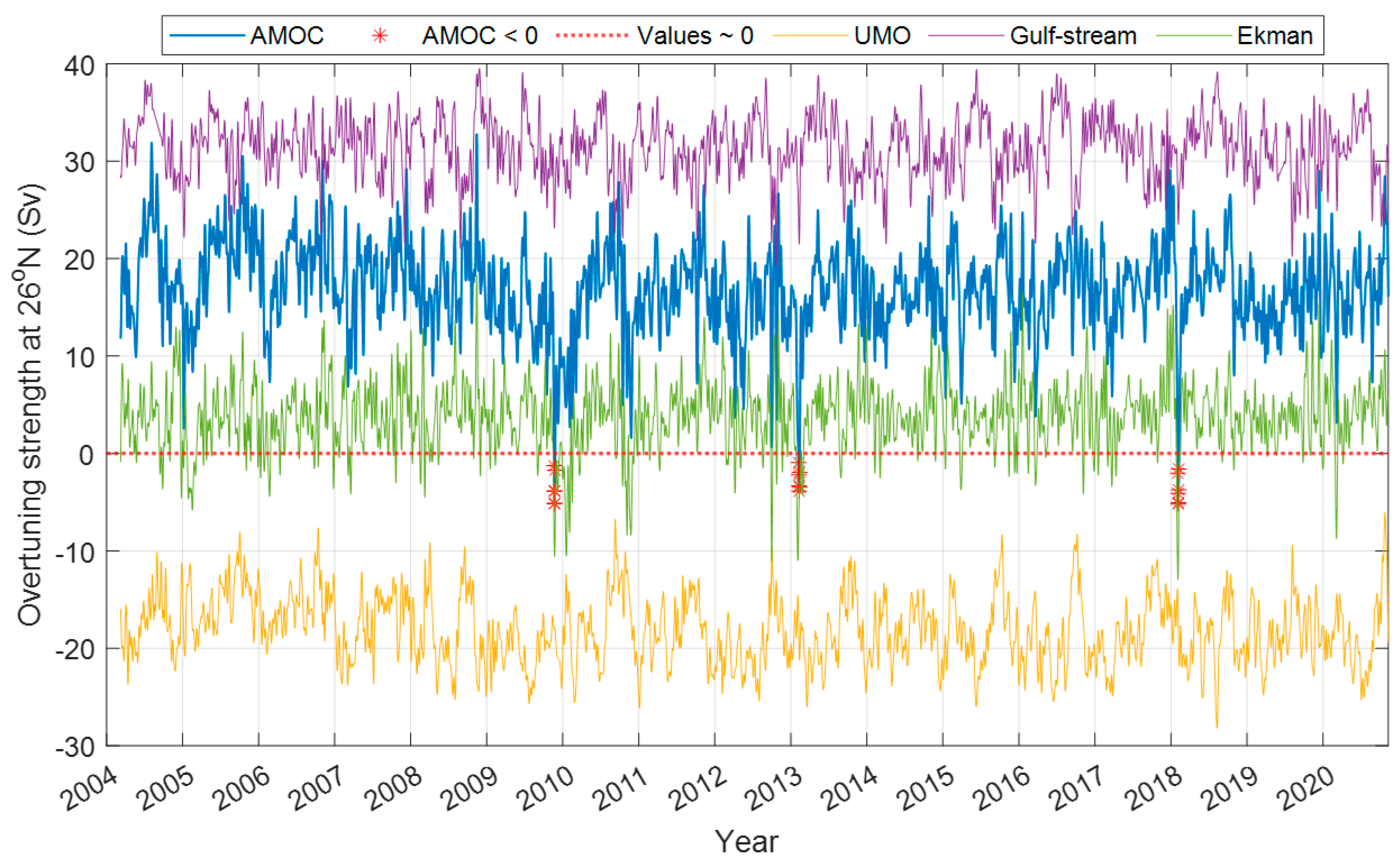
First, the variability of the AMOC transport using the latest existing recordings is explained using two approaches. Initially, the AMOC is divided into its components, i.e., Florida current (GS transport), meridional Ekman transport, and upper mid-ocean (UMO) transport between the Bahamas and the Canary Islands, as shown in Figure 2, in terms of overturning strength (OS in Sv) versus year. GS transport (always observed positive) is based on electromagnetic cable measurements; Ekman transport (observed as sometimes negative) is based on the interaction between wind and ocean surface; while the UMO transport (always observed negative) is the vertical integral of the transport per unit depth down to the deepest northward velocity (~1100 m) on each day. Overturning transport (AMOC) is the sum of the three explained components and represents the maximum northward (positive values) transport of upper-layer waters each day.
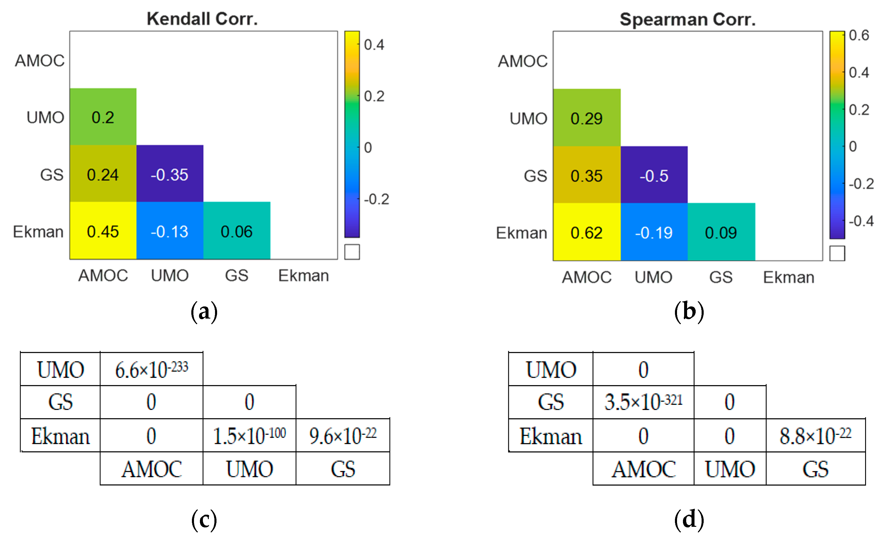
The correlation analysis between the daily time series of AMOC and its components is conducted, and the results are presented in Figure 3. Figure 3a displays Pearson coefficients at zero lag, Figure 3b shows the corresponding p-values, and Figure 3c illustrates the maximum or minimum lagged-correlation values. All Pearson coefficients in Figure 3a have p-values that are very close or equal to zero indicating statistically significant. These p-values are smaller than the significant obtained level of 3.24 × 10⁻²⁸, corresponding to a confidence level of 100 × (1–3.24 × 10⁻²⁸)~100%. Therefore, the observed correlation values are considered significant. The results reveal the highest positive similarity between AMOC and its Ekman component as +0.69 at zero lag (with a p-value of zero) and as +0.692 for a one-day lead. This shows a strong direct impact of the Ekman component, which represents wind stress, in transporting heat into the AMOC during the daily periods. This finding is consistent with a previous study [44] that also confirmed this relationship for periods shorter than two months. Additionally, the maximum negative correlation (minimum) of −0.52 at zero lag and −0.552 at a one-day lag is observed between the GS and UMO. These components flow in two different directions and the negative correlation is also supported by [44] for timescales shorter than 1 year. Furthermore, Figure A1 in Appendix A presents the results using two alternative methods to calculate correlations: Kendall and Spearman. The Pearson and Spearman methods yield almost similar results, while the Kendall method shows lower correlation values in comparison.
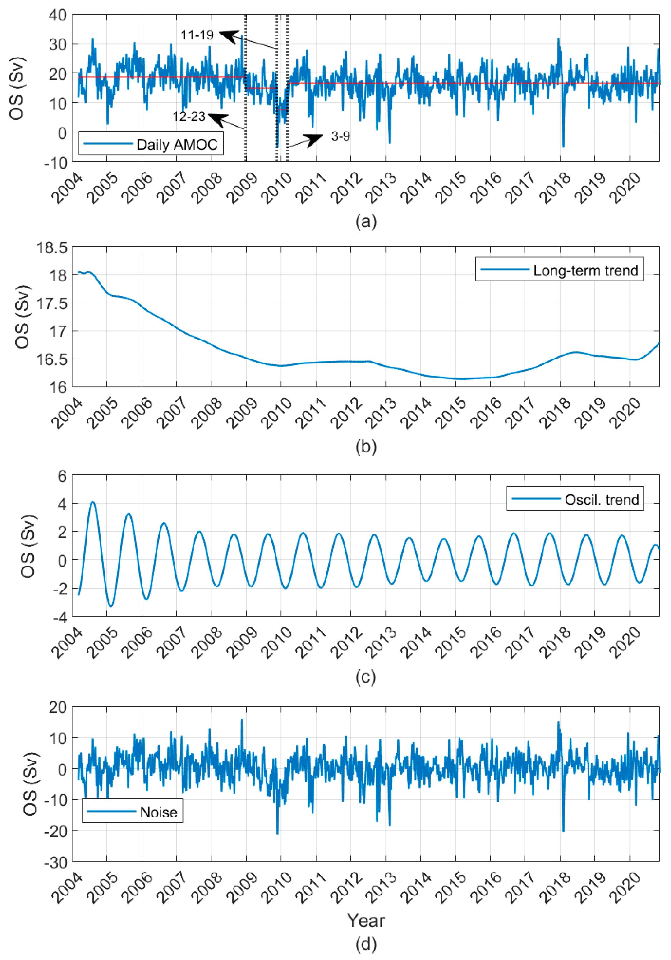
In the second kind of AMOC analysis, the AMOC measurements (Figure 4a) are decomposed into three parts according to the SSA method mentioned in Section 3: a long-term trend, a seasonal trend, and the residual (noise) signal as shown in Figure 4b–d, respectively. Additionally, the analysis of critical change points (this method finds the years in which the AMOC change most significantly in terms of the mean value [53,54]; in this way, the AMOC variations can be divided into a finite number of regions (selected by the user as far as is possible by the algorithm in [53]), and the sum of the residual (squared) error from its local mean can be minimized for each region separately) identified three critical years (Figure 4a) and four different time windows (with different mean values over that period): the beginning of 2009, the end of 2009, and the spring of 2010. The minimum value of AMOC is observed in the interval 2009–2010. However, instantaneous minima are also recorded at the beginning of 2013 and 2018. The long-term trend (Figure 4b) shows a fast decrease from 2004 to 2009 from 18 to 16.5 Sv, followed by a slight decrease from 2009 to 2010, which remains almost constant from 2010 to 2012. Small decreases are observed from 2012 to 2016, and after that, AMOC changes its direction again toward an increase (i.e., it seems recovering), although some changes between 2018 and 2019 are also observed. However, the values at the end of the observation period (and of 2020) are still lower than the ones in 2004. The difference between AMOC values from 2004 to 2020 shows a general 7% decrease for 16 years.
If the decreasing speed remains constant, a decrease of about 20% (with low confidence) might be estimated over the first half of the 21st century. Next to [14,15,16,17], which show the weakening of AMOC at a fast rate over the 20th century or within the last 50 years, ref. [21] has predicted a 20% weakening of the AMOC during the first half of the 21st century and a stabilization and slight recovery after that. The seasonal variations in AMOC are cyclic, with a decreasing magnitude before 2009 and a constant magnitude after that. The high-frequency variations have shown a minimum value of −21 Sv and a maximum of +15 Sv, as shown in Figure 4d. However, the range of noise values changes mostly from −10 to +10 Sv, which is similar to the 10-day measurements in [44] for the period of 2004–2018.
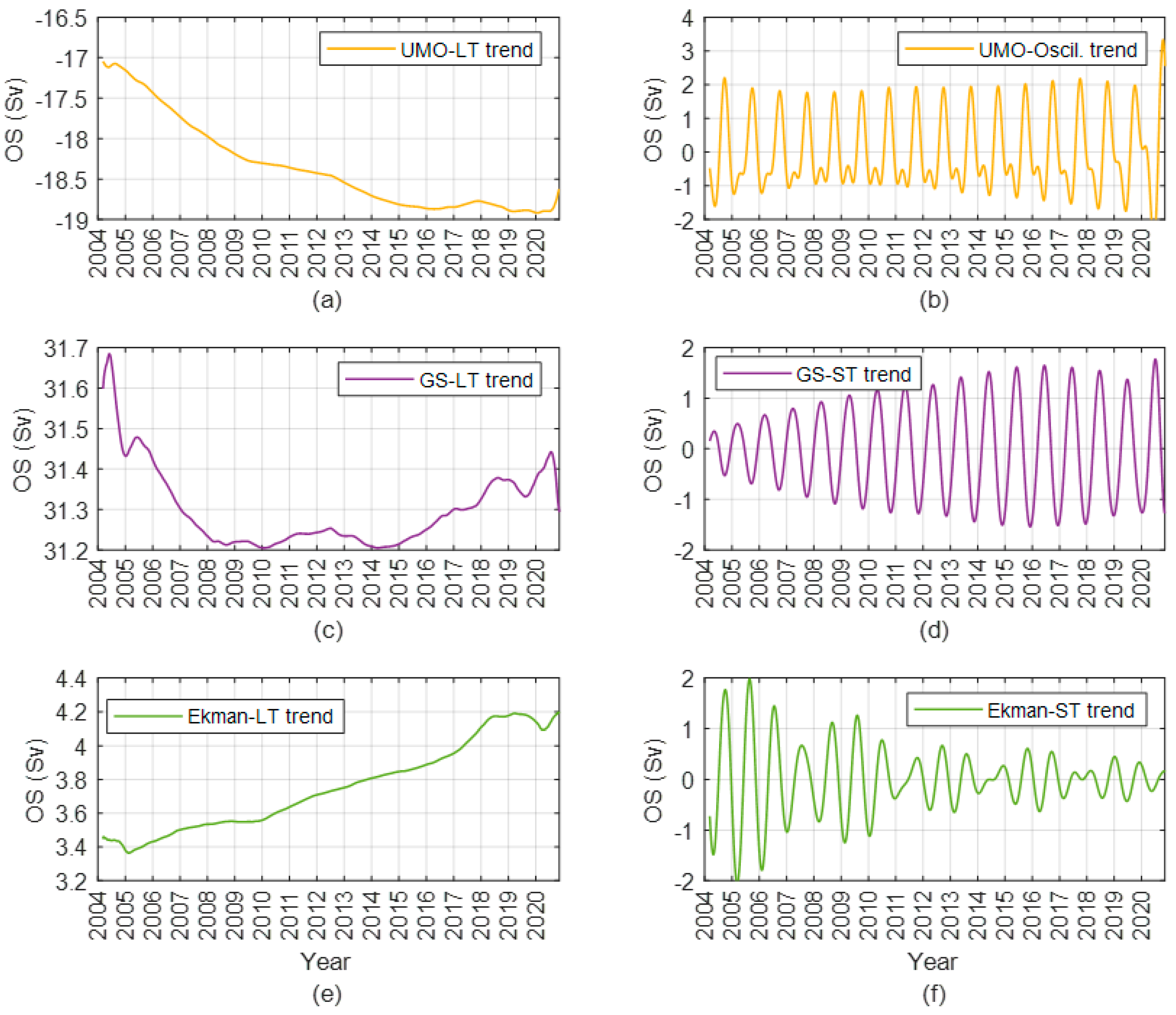
Figure 5 shows the long-term and seasonal variations for AMOC components. The general long-term trends show GS weakening (or at least decreasing), as well as strengthening of Ekman, and strengthening of UMO in its negative direction (weakening in the positive direction). However, the behavior is different for the periods after 2017–2018. The “GS weakening in the same direction as AMOC” and the “strengthening of UMO in the opposite direction” are the main key for the AMOC weakening, despite Ekman increasing, as observed in Figure 4b and Figure 5a,c,e. Although a high correlation is observed between daily measurements of AMOC and Ekman (Figure 3), it is clear (Figure 4b and Figure 5a) that AMOC is governed/dominated by UMO. This result was also confirmed in [44] for time intervals longer than a year (our case, daily from 2004 to 2020). The minimum value of GS was observed around 2010. The cyclic variation for the three components also shows that the behavior before 2009–2011 is different from that after that period.
To examine the anomalies within the AMOC variations and its components, a yearly average (based on the daily time series shown in Figure 2) along with its corresponding yearly standard deviation is depicted in Figure 6. The results in Figure 6 are more similar to the results published in (Figure 4, [44]) for the AMOC and its component’s interannually variability than to long-term trends in Figure 4b and Figure 5a,c,e, in which the SSA algorithm is applied by employing SVD analysis on the trajectory matrix including lagged sub time series for each of AMOC and its components, separately. The mean and standard deviation for the different transports in the year 2020 and after that are 17 ± 4.3 Sv (AMOC), 31.3 ± 3.2 Sv (GS), 4.3 ± 3.4 Sv (Ekman), and −18.5 ± 3.7 Sv (UMO). The minimum values of AMOC are observed first for 2009–2010 and then for 2010–2011, as dashed vertical red lines in Figure 6a. The first decline period corresponds to the UMO, and the latter corresponds to Ekman. In 2019–2020, another local minimum for AMOC was also observed, corresponding to the year regarding the lowest value of GS. Another observation is the decreasing value for AMOC and UMO before 2009 and the recovery after that.
Note that although the long-term trend of AMOC (Figure 4b and the results presented in [44]) from 2004 to 2020 shows a small recovery after 2014, the under-study interval is from 2004 to 2020 (according to the availability of data in RAPID AMOC program for 17 years); hence, the trend looks somehow similar to averaged variations for a defined window (Figure 6a). Considering more data on AMOC and GS, which is essential in the SSA algorithm, would conclude more precise results for a long-term trend so that the recovered part is negligible. Moreover, a light decrease in AMOC is observed in 2012 and 2014, and a more severe decrease is seen in 2019, as shown in Figure 6a for the winter AMOC. The AMOC trend can be seen as an almost constant trend followed as weakened, such as the results presented in [35], in which three periods are divided for AMOC strength: before 2000 (almost constant), 2000–2020 (weakening), and 2020–2050 (forecasted weakening with more strength). We aimed to investigate and confirm whether the AMOC is weakening in a general sense based on the available data.

4.2. Winter Temperature Variations at Candidate Locations

This section provides an analysis of winter temperature variations in the selected locations using two approaches:
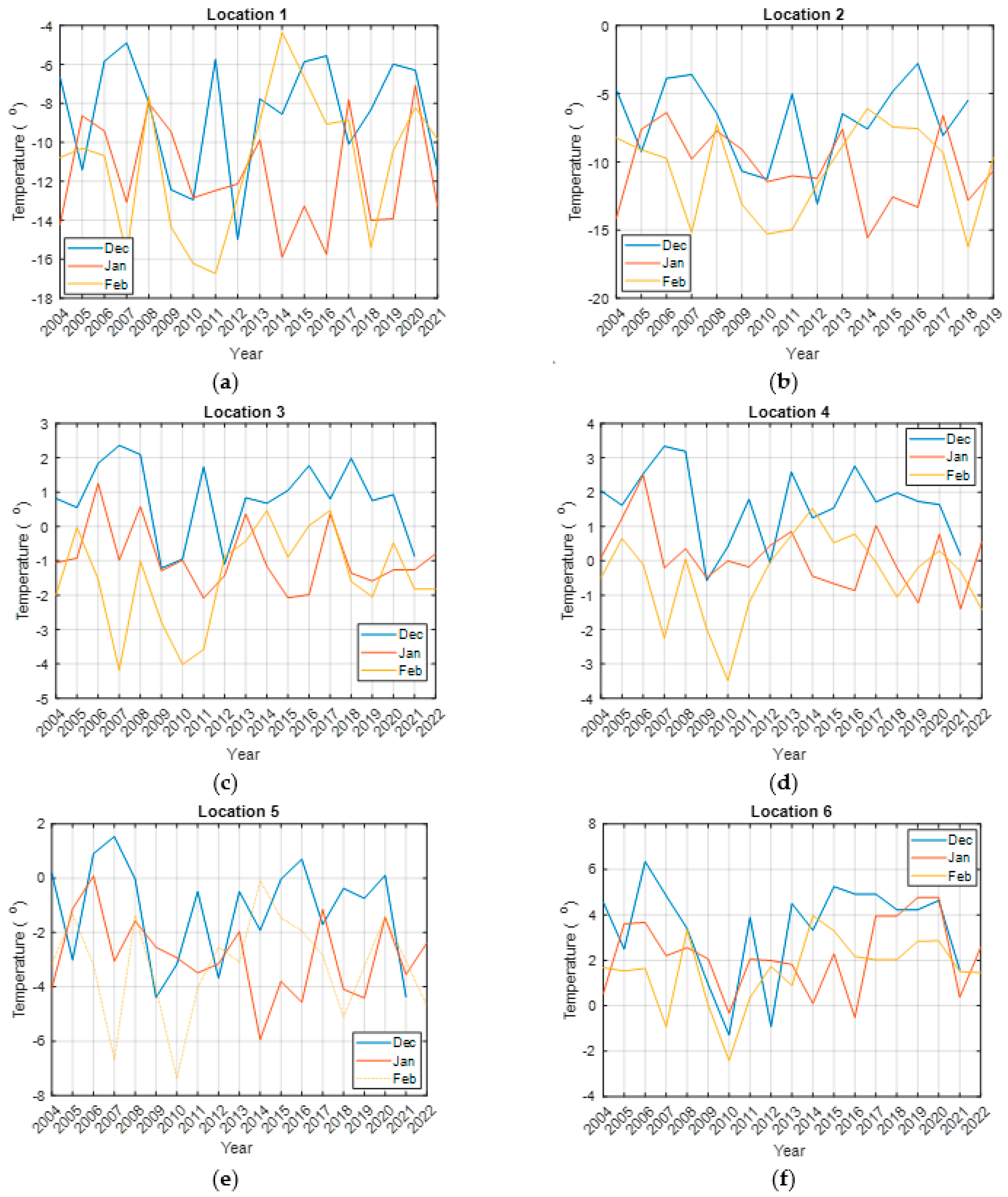
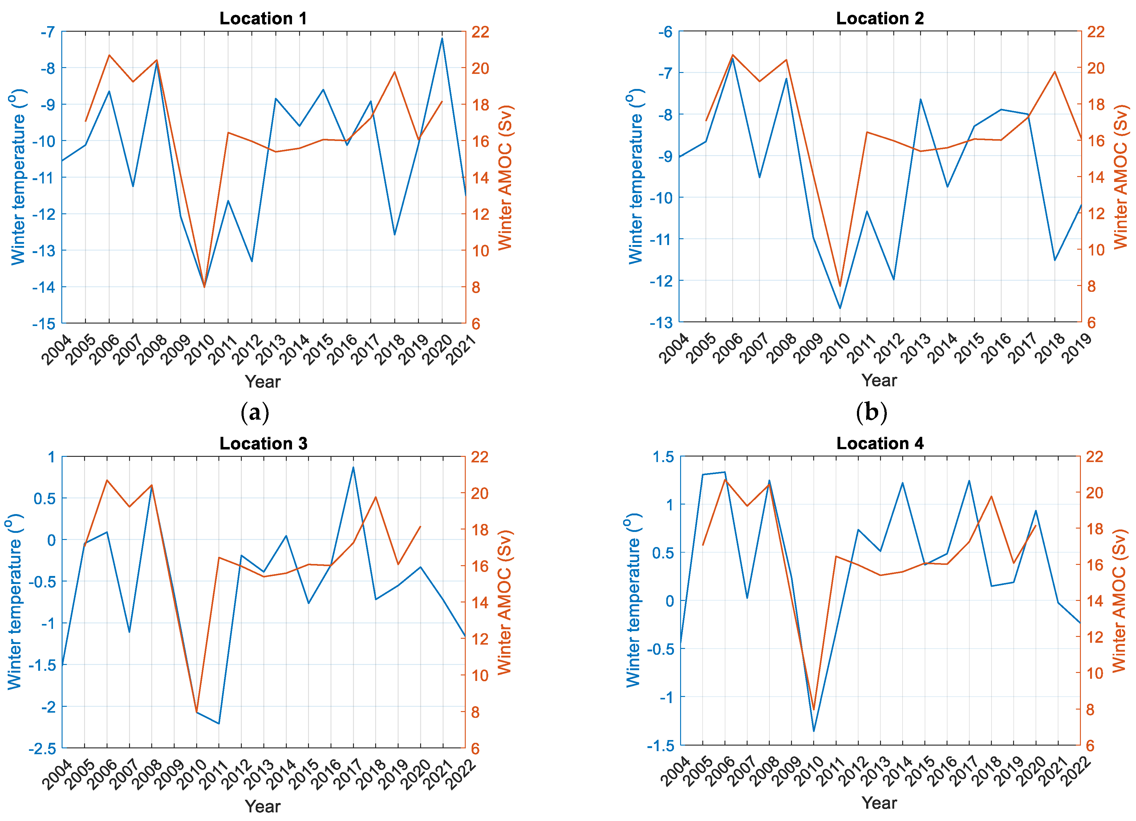
(a) An investigation of anomaly detection for all winter months through a yearly average analysis. This analysis covers the period from 2004 to the present, depending on the existing temperature data and considering the availability of AMOC data (Figure 7).
As shown in Figure 7, clearly, the winter months in locations 1 and 2 in Sweden are much colder than the other locations in Norway. The winter temperatures over the years can be divided into three periods: when February is the coldest month (before 2012), when February is becoming warmer, some years even the warmest month (2012–2017), and when February is close to January temperatures (after 2017). It also shows that February is somehow becoming warmer over time in the selected locations. The local minima are observed in 2007, 2009, 2010, 2012, 2018, and 2019. These anomalies in minimum values are clearer in February. Looking at the yearly average of December, specifically for locations 3, 4, and 6, shows that there is a downward trend before 2010, an upward after that, and again downward till the end of the observation period.
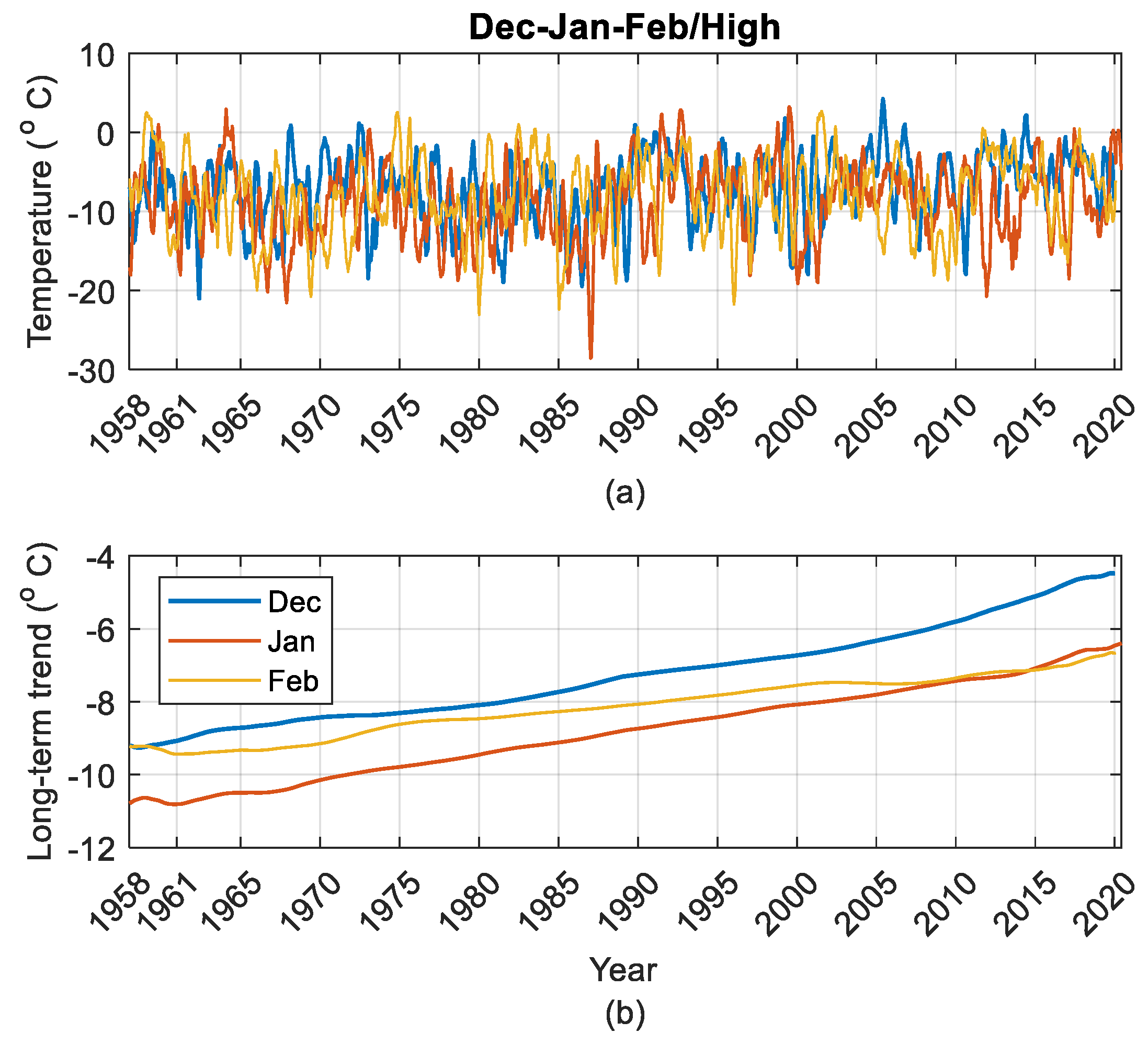
(b) A long-term analysis of temperature variations, focusing on daily lowest, highest, and average temperatures for all winter months. This analysis spans a period of at least 50 years and, at most, 71 years (Figure 8, Figure 9, Figure 10, Figure 11, Figure 12 and Figure 13 and Table 2). The SSA’s capabilities in noise reduction, localized trend analysis, interpretability, and handling missing values and outliers (for example, the values at the connection point of two similar months over different years in the temperature time series) make it a powerful tool for extracting long-term temperature trends that may not be achievable with traditional methods.
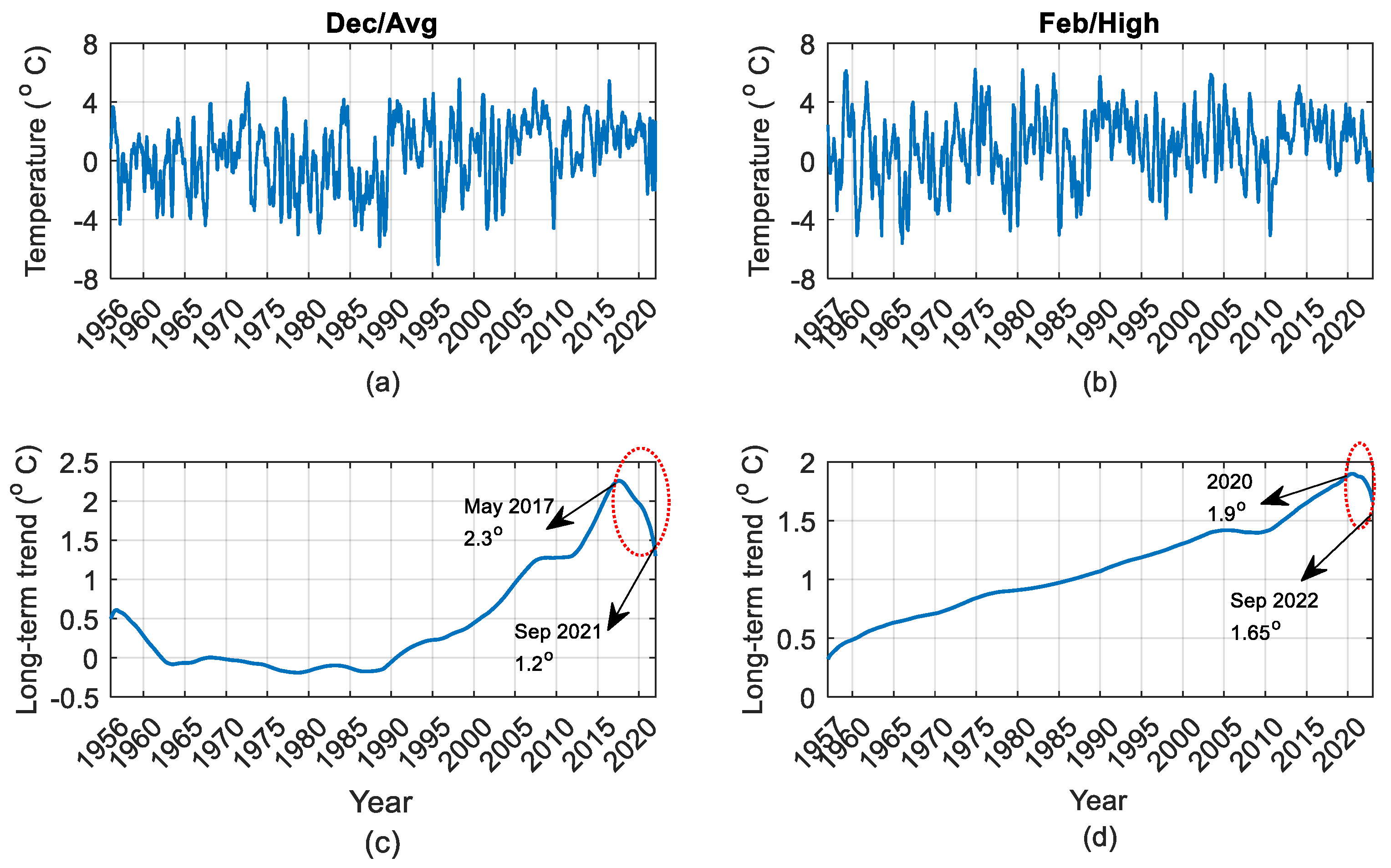
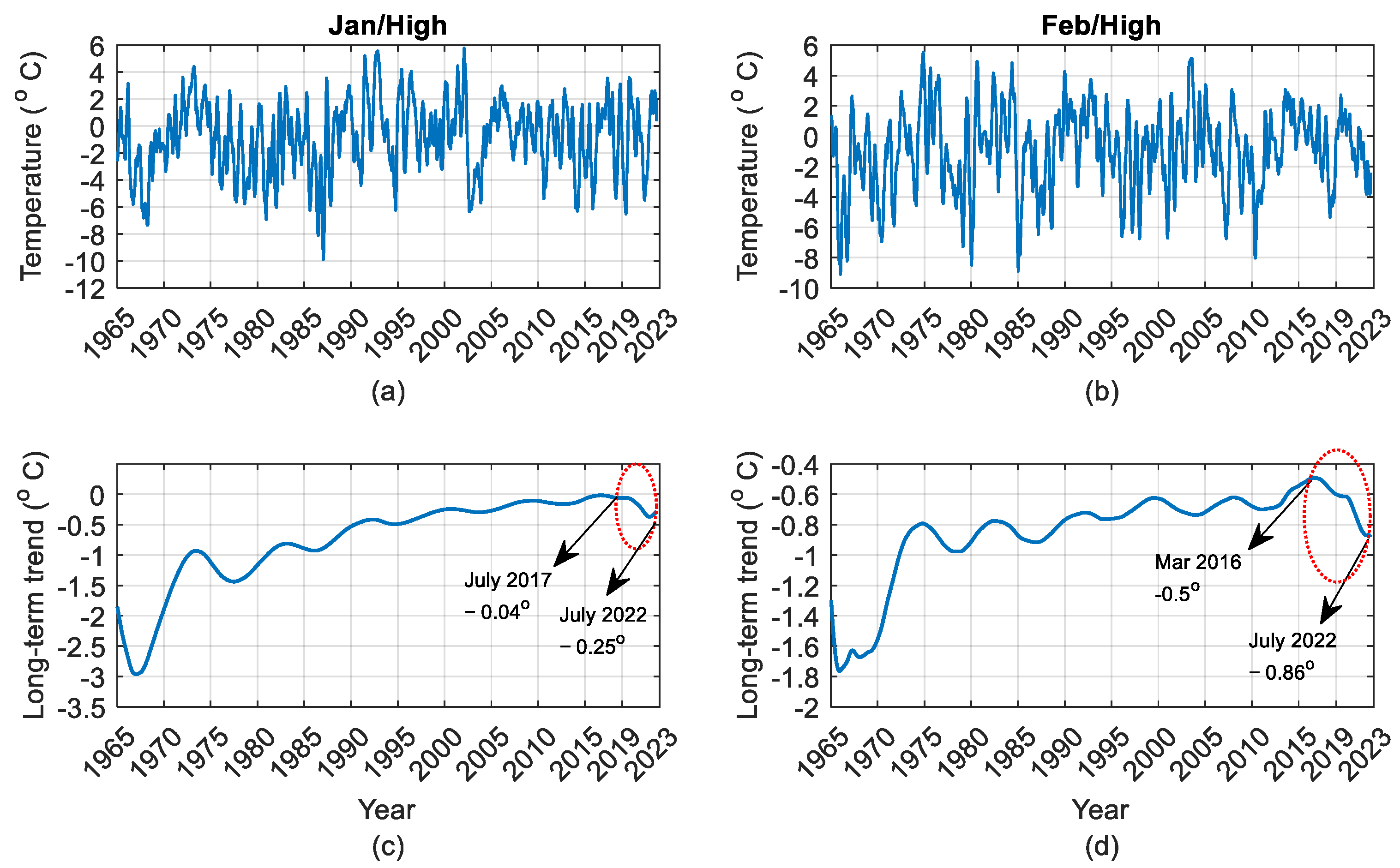
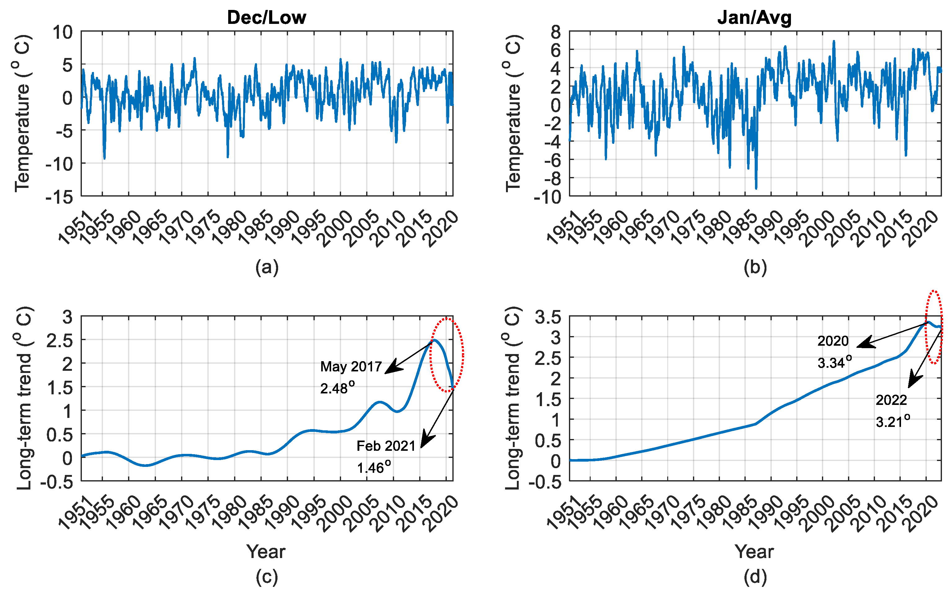
Figure 8, Figure 9, Figure 10, Figure 11, Figure 12 and Figure 13 showcase a chosen set of temperature plots for each location, with a specific emphasis on the highest temperatures. These plots represent a selection from various potential combinations, including average, highest, and lowest temperatures, for December, January, and February, a total 6 × 3 × 3 = 54 time series. The long-term trend of December/January/February highest temperatures in location 1 for 63 years from 1958 to 2020 (Figure 8b) shows an increase with a constant slope from −9.5 to −5 °C (December), −11 to −7 °C (January), and −9 to −7 °C (February). This location seems to be affected more by global warming since the long-term trend is just increasing.
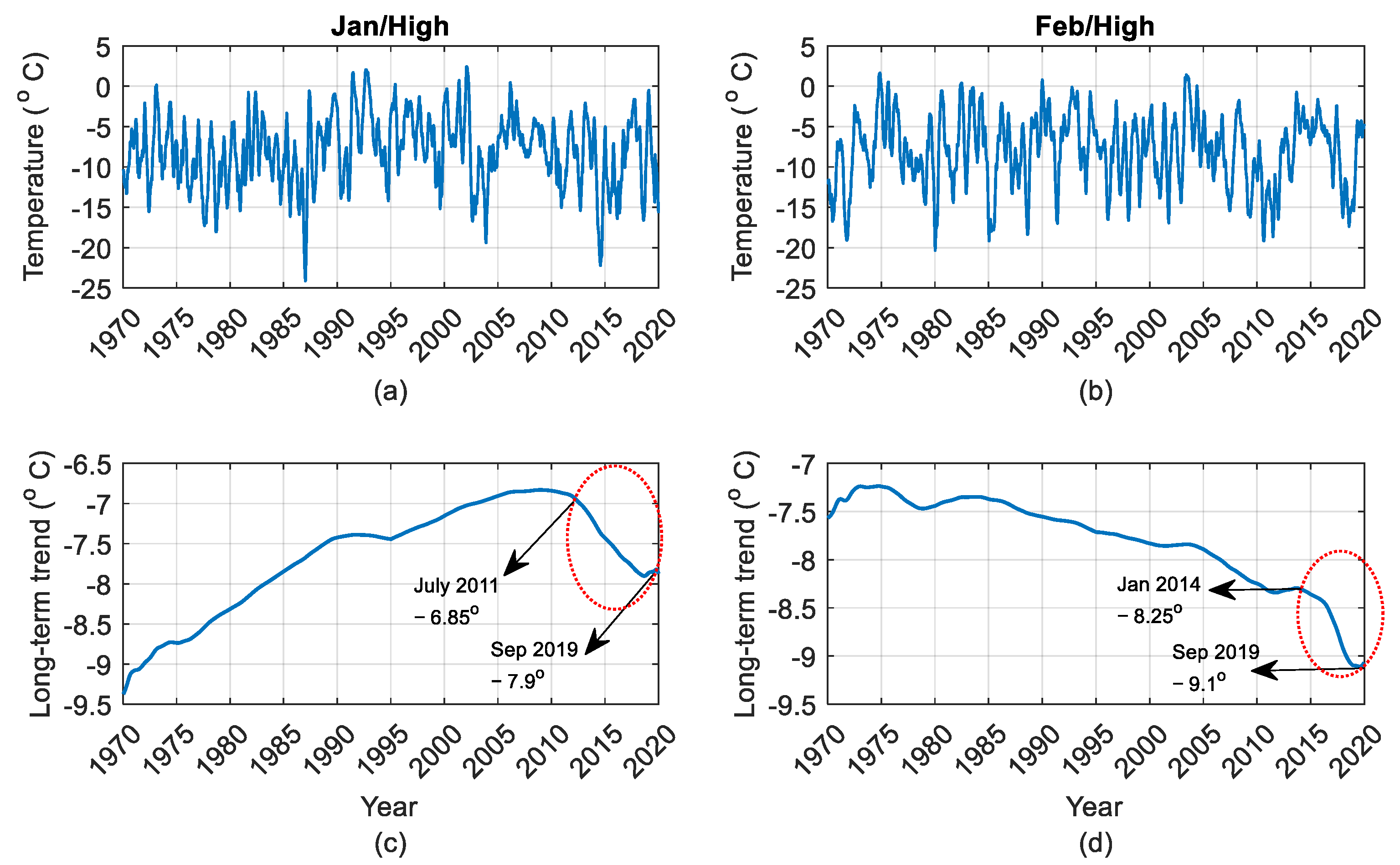
Figure 9a shows the highest temperatures for January in location 2 (northwestern Sweden). The long-term trend (Figure 9c) shows the increased temperature from −9.5 (1970) to −6.85 °C first (around 2011) affected by global warming (+2.15 °C increasing in 42 years). Between the end of 2011 and the end of 2019, the temperature decreased from −6.85 to −7.9 °C, as indicated by an ellipse in Figure 9c (−1.05 °C decreasing in 9 years). The downward part may be attributed to specific reasons. A possible scenario is explained here. According to the results of some of the literature, such as [35], in which a broad range of AMOC variations are studied and show AMOC weakening (and also the general view of AMOC in Figure 4b, which shows weakening), the marked area, which has a faster speed of decreased temperatures than the increased temperatures before that, may show a possible role of AMOC weakening. Note that the direct impact of global warming is the warming and increasing temperatures; however, an indirect impact is on the AMOC weakening, which, by itself, has the task to transfer warm surface water. Moreover, the speed of AMOC weakening has been confirmed more often than the speed of global warming [35]. Nevertheless, these observations could not be detected by the yearly average temperatures shown in Figure 7b from 2004 to 2019. Figure 9b shows the highest temperatures for February in location 2. The long-term trend (Figure 9d) shows, first, some small variations by 2005. Between 2005 and 2010, the temperature decreased and then increased until 2014. After that, a clear decrease in temperature is seen from −8.25 °C to around −9.1 °C by the end of 2019, as indicated by an ellipse in Figure 9b. The observations for the marked period could be also detected by the yearly average temperatures shown in Figure 7b from 2014 to 2019.
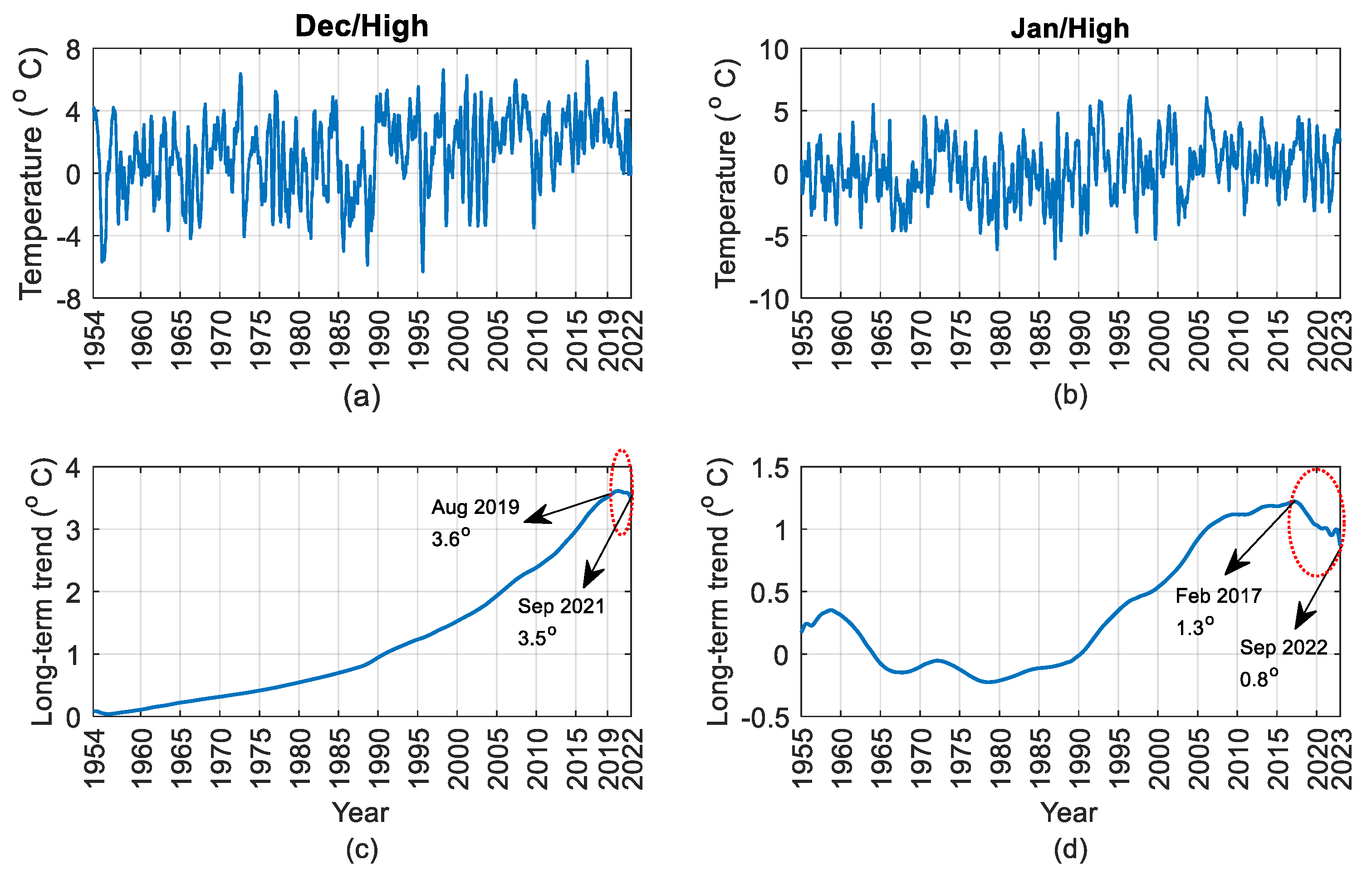
Figure 10, Figure 11, Figure 12 and Figure 13 show the daily temperatures for locations 3 to 6, respectively. From the first year of study to around 2017/2019 (for location 3), 2017/2020 (for locations 4 and 6), and 2016/2017 (for location 5), there is a slight (linear/nonlinear) upward long-term trend. This is followed by a downward trend, shown by an ellipse in Figure 10c,d, Figure 11c,d, Figure 12c,d and Figure 13c,d.
An analysis of the results from the six locations (some of which are depicted in Figure 8, Figure 9, Figure 10, Figure 11, Figure 12 and Figure 13) reveals a general long-term temperature trend indicating an increase, which can be attributed to global warming. However, it is noteworthy that 50% (27) of these various combinations of long-term trends have shown a considerable decrease in recent years. Additional details regarding the downward long-term temperature trends are presented in Table 2. The rates of decreasing temperatures, represented as slopes of linear trends, are sorted by color in the column before the last one. In this column, December exhibits the highest decreasing rate in locations 4 and 6. The average rate of change in decreasing temperatures per location is as follows: 0.09, 0.04, 0.088, 0.059, and 0.076 °C/year for locations 2 to 6, respectively. As seen, locations 2, 4, and 6 have experienced colder temperatures in recent years. In order to further examine the underlying factors contributing to the observed downward trends in long-term winter temperatures, indicating the possibility of colder winters in recent years, a thorough and detailed analysis is required. This investigation should involve studying temperature change maps and conducting analyses to establish connections between potential causes and the decrease in temperatures, as well as explaining why these effects are particularly prominent in December and vary across different locations. While multiple factors could contribute to these downward trends, Section 4.3 and Section 4.4 will provide valuable insights into two significant climatic indices, namely, AMOC and NAO, as potential explanatory factors.

4.3. Possible Similarity between Winter Variations in AMOC and Temperatures of Candidate Locations

Previous research, including the study referenced as [58], has demonstrated that a 1 Sv alteration in the AMOC can lead to approximately a 0.3 °C change in SSTs for decadal-centennial changes, i.e., a 0.03 °C/(year. Sv). Moreover, these studies have also identified similarities in the variations of AMOC and SSTs. However, they did not pay attention to the regional winter temperatures affected by AMOC variations.
In a more recent investigation [59], an artificial weakening of the AMOC was conducted, reducing it by an average of 57% over 60 years, equivalent to an average of 7.55 Sv, i.e., a 1 Sv weakening for 7.94 years. The results indicated that a weakened AMOC has a cooling effect on the global near-surface air temperature in the Northern Hemisphere, with an average decrease of −1.09 °C/year to −0.14 °C/(year. Sv). The majority of cooling occurs in the Northern Hemisphere, which experiences an average temperature decrease of −2.09 °C/year to −0.26 °C/(year. Sv). Notably, the most significant changes are observed during winter, with a cooling effect of −2.42 °C to −0.3 °C/(year. Sv). These findings suggest that other factors, such as regional warming/cooling, can also influence the magnitude of cooling associated with a weakened AMOC. However, it is important to note that the analysis in the study [59] is conducted using artificially weakened AMOC simulations and climate models, rather than real observational data.
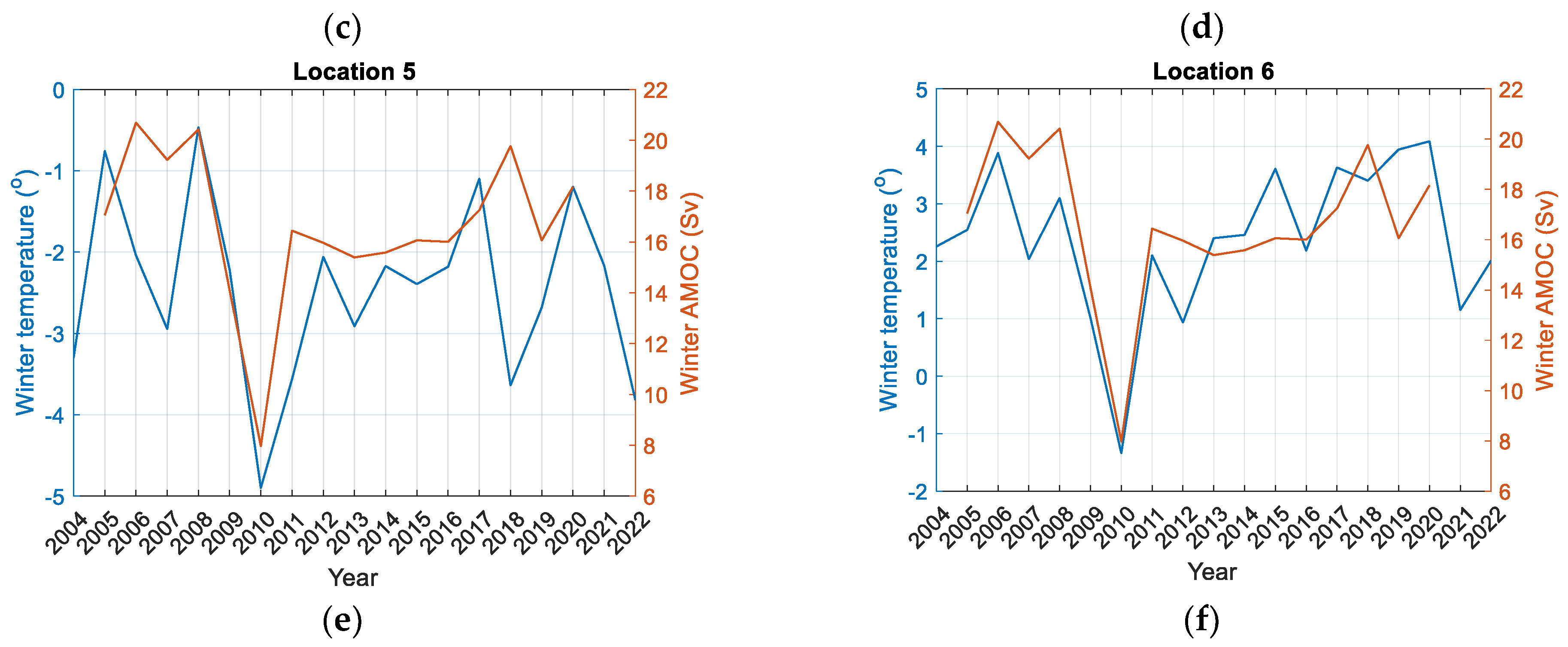
With the information derived from the previous paragraph, this section examines the possible similarity between winter variations in AMOC and winter average temperature variations in the selected locations. Figure 14 illustrates the yearly average variations in AMOC and temperatures at the locations throughout the entire winter season. This analysis covers the period from 2004 to the present, depending on the existing temperature data and considering the availability of AMOC data, which covers from April 2004. The observations from Figure 14 reveal the winter AMOC deep anomalies in 2010 and 2019. The yearly average winter temperatures across all locations indicate a synchronized response to the winter temperatures without any time lag before 2010. Notably, the light and deep minima observed in AMOC in 2007 and 2010, respectively, coincide with the winter temperature minima. From 2010 to 2016, specifically for locations 3 to 6, a slight positive lag can be observed between the AMOC and temperatures. However, starting from 2016 onwards, it appears that there is a larger time lag between smaller AMOC variations and larger variations in temperature. It is also noteworthy to pay attention to the local minima of AMOC in 2018, which is followed by a decrease in temperatures with a lag observed in locations 3 to 6.
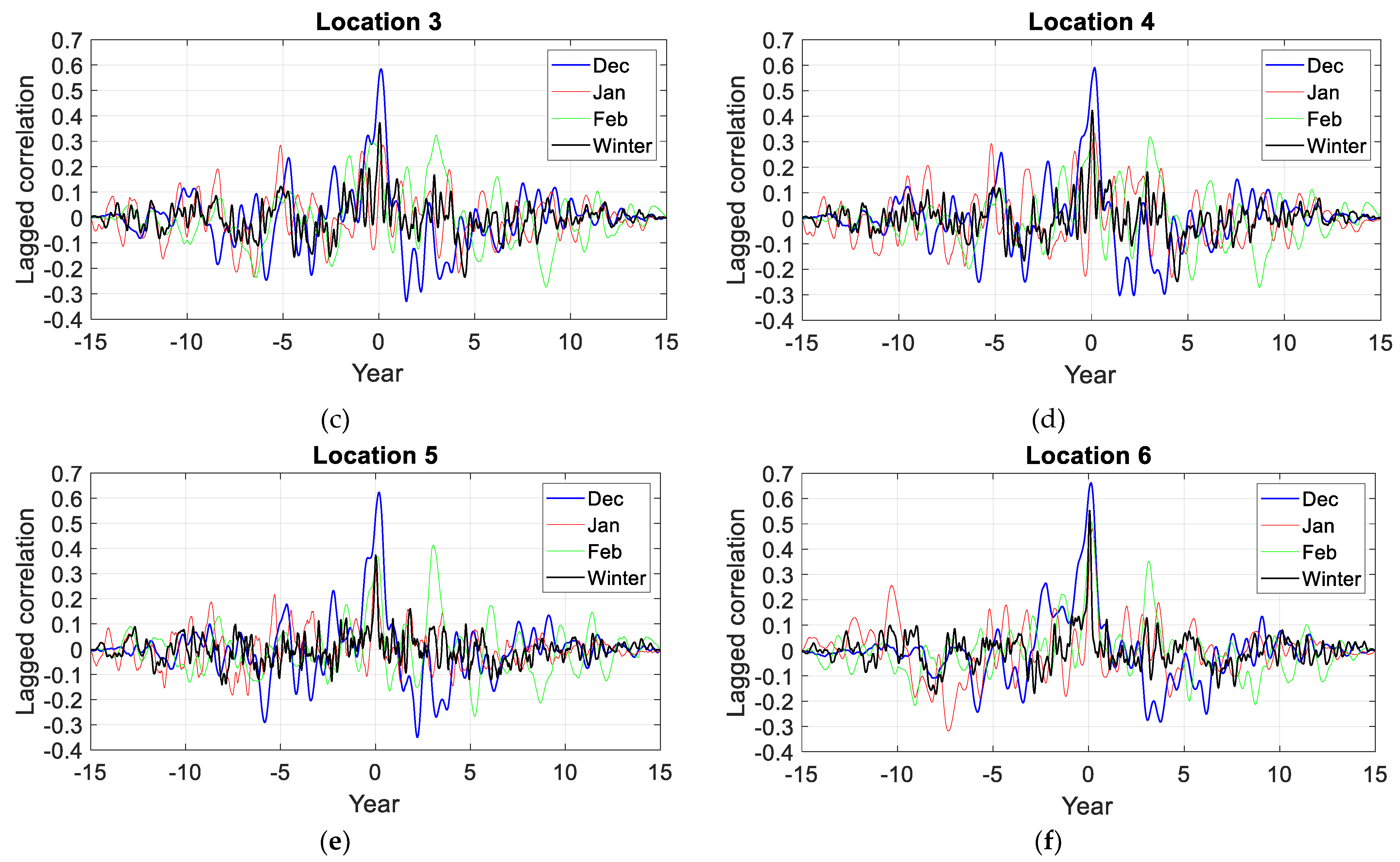
The highest lagged correlation along with their corresponding lag values between winter AMOC and average temperatures time series spanning from 2005 to 2020, are presented in Table 3. Almost the same results were concluded for the highest and lowest temperatures. In general, all computed correlation values are higher than 0.2 for the average temperatures; however, December exhibits the highest correlation among the winter months with the AMOC variations. Specifically, locations 4, 6, and 3 demonstrate the strongest correlations (0.58, 0.52, and 0.49) compared to the other locations. The lag values increase from locations 1 and 2 to 3 and 4, and further to 5 and 6. From Table 3, the maximum lagged correlations are notably 0.49 and 0.58 at a lag of 0.065 years (approximately 24 days). For the entire winter season, the highest correlations and the corresponding lags are observed in locations 3, 4, and 6 as 0.32, 0.37, and 0.43 with the lags 28, 20, and 12 days, respectively. The lag values decrease from locations 3 to 6, while almost no lag is observed for locations 1 and 2.
The results from Figure 14 and Table 3 show (1) The possible contribution of AMOC (indirect most likely) to colder winters locally around 2010, and further, due to the positive lagged correlations between AMOC and winter temperatures. It should be noted that there is a decrease observed in 2018–2019 in Figure 14. Although there is no available information for 2020–2022, according to reference [53], there is a possibility of a decreasing trend in AMOC during that period. (2) Higher correlations between winter AMOC and temperatures (>0.49) are observed specifically in December, for locations 3, 4, and 6. (3) There is a pattern where the correlation value increases and the corresponding lag decreases from location 3 to 4 and then to 6, which are those areas along the southern part of the coastline of Norway. There is a clear pattern where the correlation value increases and the corresponding lag decreases from location 3 to 4 and then to 6.
The objective of this study is not to quantify the exact magnitude of temperature decrease resulting from changes in AMOC strength but rather to determine if there are considerably lagged correlations between them. Our focus has primarily been on the impact of AMOC weakening in low latitudes on colder winters in mid to high latitudes, even though an AMOC strengthening would be observed for high latitudes [60] linked to colder winters. According to Table 2, locations 3, 4, and 6 experienced an average temperature decrease of −0.04 °C/year, 0.088 °C/year, and 0.076 °C/year, respectively. In a simple analysis, one could consider that an AMOC weakening of 1.3 Sv, 2.6 Sv, and 2.53 Sv, based on the findings in [58], or 0.28 Sv, 0.63 Sv, and 0.54 Sv, based on the findings in [59], might have contributed to these temperature decreases. Based on the findings of this section, it can be concluded that the weakening of AMOC around 2017 played a significant role in reducing the transfer of warm surface waters. However, despite observing a moderate correlation, establishing a direct link between winter AMOC and temperatures, as well as identifying the mechanisms through which AMOC impacts temperatures on daily/monthly timescales, proves challenging. Nevertheless, there may still exist, with a lesser degree of certainty that necessitates further investigation, a potential connection between winter AMOC and winter temperatures in mid to high latitudes, as well as a potential link between winter AMOC and the downward patterns observed in Table 2. The next section will focus on examining another variable that may influence winter temperatures.

4.4. Possible Impacts of Other Variables, Particularly NAO, on the Winter AMOC and/or Temperatures

The moderate correlations observed between winter AMOC and temperatures (Section 4.3) may not necessarily imply a direct causal relationship. It is possible that a third variable, such as wind or the NAO, influences the AMOC, the temperatures, or even both. The previous study [23] explored the relationship between GS weakening, AMOC weakening, and the NAO decline in 2010, confirming the connection between AMOC weakening and NAO reduction. Additionally, it has been observed that NAO+ (positive phase of NAO) strengthens the AMOC on timescales exceeding 20–30 years [12]. Research conducted on various mountain cities in Europe, Morocco, Turkey, and Lebanon in 2011 indicated that projected NAO trends could lead to increased winter modes and a decrease in the number of cold winters during the 21st century, due to the influence of global warming [61]. The direct impact of NAO+ on the warm summer in 2018 was also demonstrated [13]. The spatial variability of NAO has been found to play a crucial role in regulating the European climate in addition to its temporal variability [62].
In addition to the factor of AMOC weakening, it has been observed that the AMOC exhibits a strong response to wind-driven variability, particularly by the Ekman component, which is in turn influenced by the NAO. During NAO+, stronger winds over the subpolar North Atlantic increase surface heat loss to the atmosphere, promote the formation of dense water, and result in a strengthened AMOC [63]. A study conducted in [44], utilizing AMOC anomalies from the RAPID and GloSea5 datasets at 26° N, along with Atlantic indices such as NAO, examined the relationship between NAO phases and various parameters. It was found that during an NAO (NAO+) state period, there is a reduction (increase) in surface heat loss and weakening (strengthening) of winds over the subpolar North Atlantic, resulting in a weaker (strengthened) AMOC. Consequently, the transport of heat by AMOC toward the northward direction decreases (increases), leading to a cooling (warming) effect on the North Atlantic, and possibly the Norwegian Sea. This aligns with a delayed decrease (increase) in SST. Hence, a clear link between NAO, winds, AMOC, and SST is established. A study conducted by [64] examined the influence of winds on the AMOC. They proposed a fully-coupled climate mode where nudging winds poleward of 45° N, through a response from the Ekman component of AMOC, resulted in statistically insignificant trends in AMOC and SST trends in the North Atlantic. These findings were pretty consistent with the observations of AMOC from RAPID at 26.5° N. Another study [65] focused on the impact of NAO on the low-frequency variability of AMOC. The simulation results revealed that the influence of NAO varied among different models. Some models indicated less sensitivity of AMOC to NAO, while others suggested a higher sensitivity. This study also highlighted the importance of the oceanic mean state as a crucial aspect of climate change that requires improvement in models.
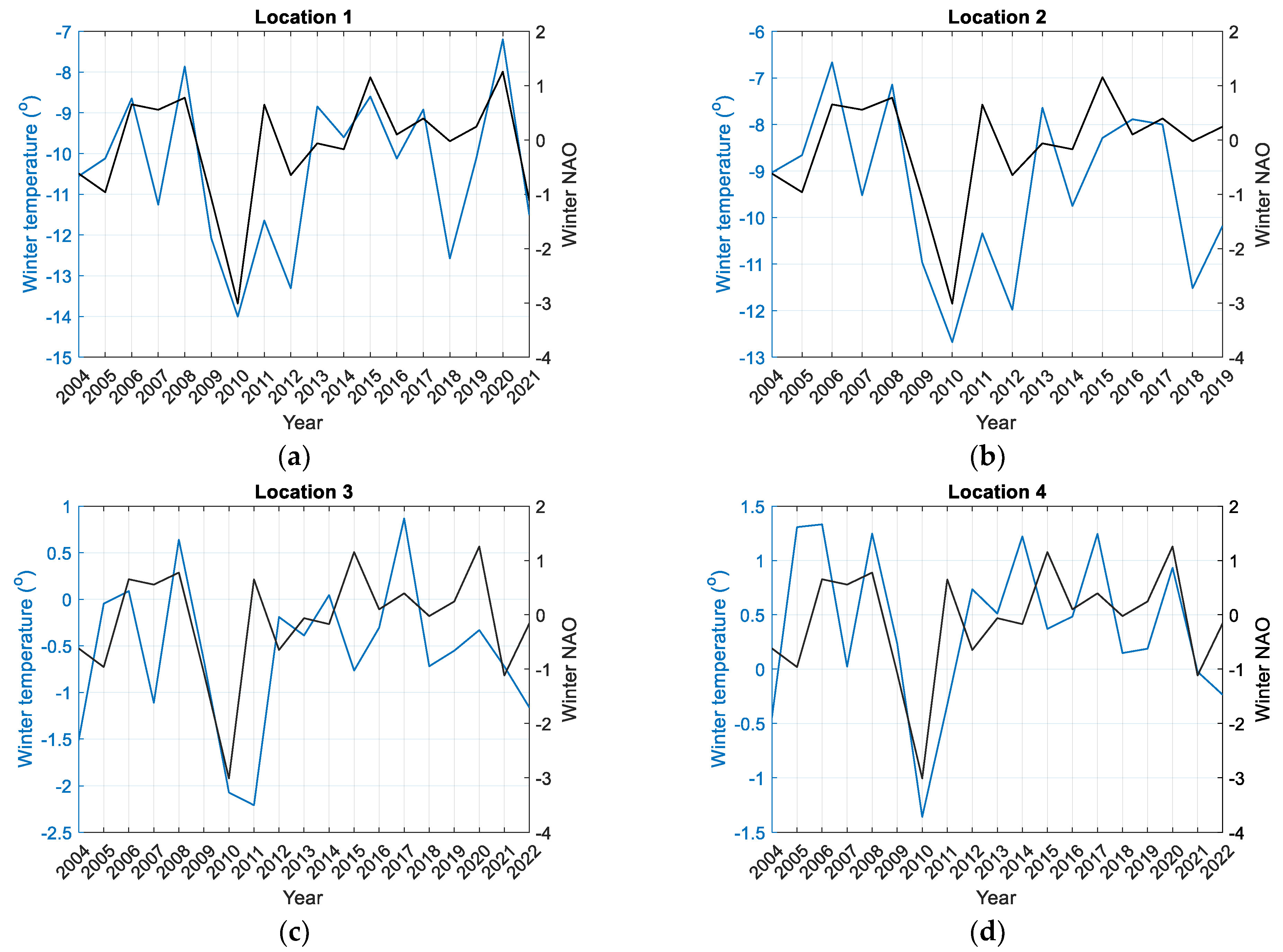
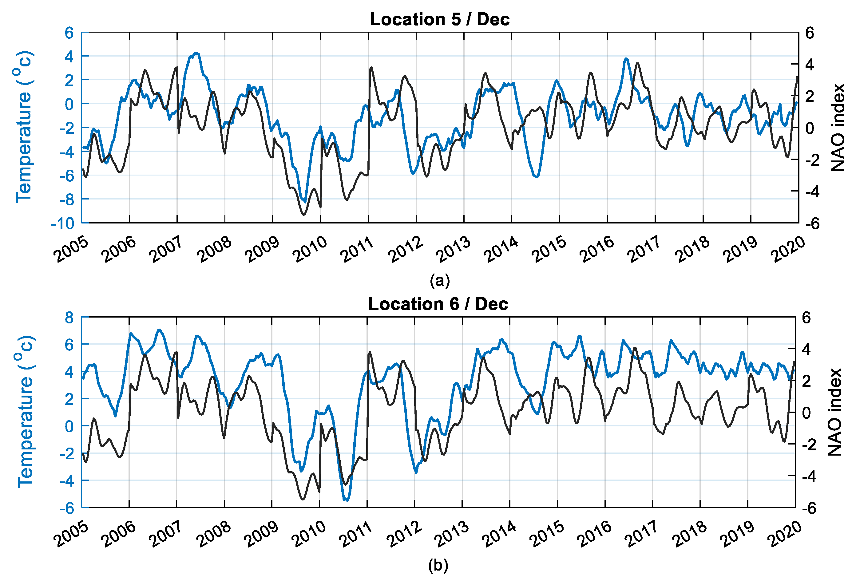
According to the literature investigated in this section, it is concluded that NAO could have affected the AMOC weakening. Hence, a possible reason for the cooler winters in the discussed locations could be due to NAO weakening (being in NAO phase for a long time). Another scenario for the cooler winters is the direct impact of NAO as attached with wind changes at those locations. Therefore, the winter yearly average of the NAO index was calculated using daily values obtained from [49]. The resulting winter yearly average of the NAO index is presented in Figure 15. The data cover a similar period as Figure 14, ranging from 2004 to the latest available year of temperature data. Observations from Figure 15 reveal the presence of deep anomalies in the winter NAO index in 2010 (corresponding to AMOC anomalies) and 2021. These are the years when the NAO anomalies align with the winter temperatures across all locations. Notably, location 6 demonstrates a clearer correlation between temperatures and NAO variations compared to the other locations.
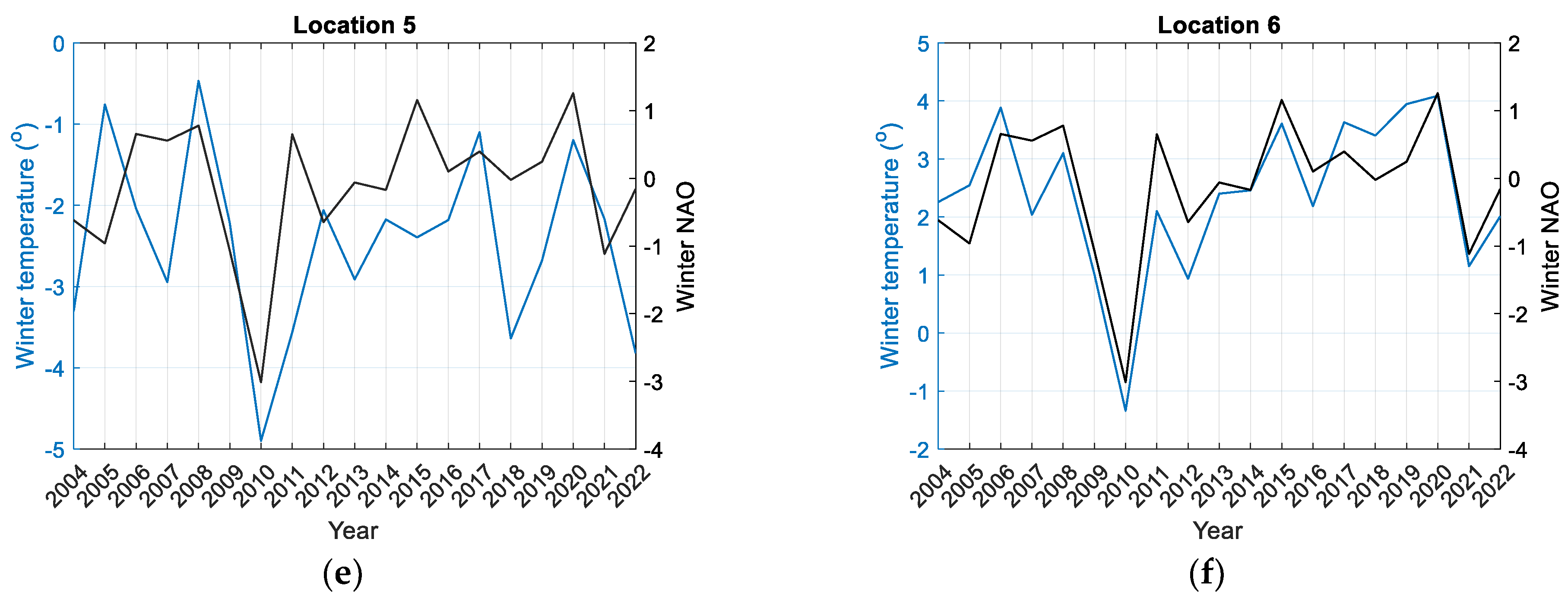
The lagged correlations between winter NAO and average temperatures time series spanning from 2005 to 2020 are shown in Figure 16. Almost the same results were concluded for the highest and lowest temperatures. Table 4 presents the highest lagged correlations between the winter NAO index and winter average temperatures, along with their corresponding lag values. The analysis is conducted both on a monthly basis and for the entire winter period spanning from 2005 to 2020, which corresponds to the same period as the AMOC-temperature analysis presented in Table 3. Overall, all computed correlation values for average temperatures are higher than 0.28. Among the winter months, December shows the highest correlation with winter NAO variations. However, it is worth noting that the correlation values between the NAO index and temperatures are higher than those reported in Table 3 regarding the possible link between winter AMOC and temperatures. Among the locations, the weakest correlation is observed in location 1 in northern Sweden, with a value of 0.57. Location 3 in the northernmost part of Norway exhibits a slightly higher correlation of 0.58. As we move to locations 4, 2, 5 (Locations 2 and 5 are in almost the same latitude positions), and 6, the correlation values increase to 0.6, 0.62, and 0.66, respectively. To illustrate this, Figure 17, as a sample, depicts the daily variations in the NAO index and temperature in December for locations 5 and 6, in which, on most days, the temperature follows the NAO with or without lag. For the entire winter, the highest correlations and the corresponding lags are observed in locations 2, 4, and 6 as 0.42, 0.42, and 0.55 with the lags 16, 12, and 20 days, respectively.
The results obtained from Figure 15 and Figure 16, and Table 4 provide insights into the possible link between winter NAO and temperatures; the following conclusions are drawn:
(1)
There is a strong relationship between winter NAO and temperatures, particularly during December, for locations 2, 4, 5, and 6. These locations, situated closer to the coastal areas of Norway rather than the northernmost regions, exhibit correlation values exceeding 0.6. Such values suggest a potentially significant influence of NAO on the temperature patterns observed in these locations.
(2)
Among locations 2, 4, 5, and 6, there is a higher probability of having colder winters influenced by the NAO for locations 2, 4, and 5. This conclusion is supported by the following observations: (i) the correlation values between the winter NAO index and winter temperatures are greater than 0.42; (ii) the highest average rates of temperature decrease in Table 2 support this pattern for locations 2, 4, and 6.
In addition to the previously mentioned factors, it is important to consider other atmospheric parameters such as atmospheric pressure, humidity, solar radiation, and wind when analyzing the temperatures over those locations. In particular, local wind speed variations, influenced by factors like the NAO or regional storm activities, could potentially contribute to the observed temperature reductions in those locations. Researchers [66] examined the connection between the winter NAO and wind climate in Norway from 1920 to 2010. The findings indicated a strong correlation between NAO+ and a higher occurrence of southwest winds from the southwest parts (such as location 6 in our study), as well as a decrease in the frequencies of northeast winds (such as location 3 in our study). However, there was no significant relationship found between the wind climate and the NAO in the northernmost part of the country (such as locations 2, 4, and 5). Therefore, based on this research, colder temperatures experienced in location 6 might also be attributed to the increased wind patterns in the area. It is also worth noting that wind simulations for certain cities in southwestern Norway (near location 6 in our study), between the 1990s and 2050s, forecast higher possible temperatures [67] around our considered period, which could mitigate the impact of local winds on observed temperatures. These findings show that further investigation and research are necessary to fully understand and explore the factors like winds, and this is an ongoing endeavor for the authors of this study.

5. Cold Winter Impact on the Electrical Power System’s Aspects

The results from Section 4.3 demonstrate a less likely relationship between the weakening of AMOC (caused by the indirect effects of climate change, specifically global warming (the direct impact of global warming is evident in the warmer weather patterns we have observed (Figure 8, for instance); however, there is also an indirect impact of global warming with a possible delay, which can weaken the AMOC; this weakening can lead to a weaker transfer of warm surface water toward the north, resulting in colder weather [59] conditions in the affected regions)) and the potential occurrence of colder winters in northwest Sweden and Norway. Additionally, there is a higher level of confidence regarding the presence of these colder winters in the coastal areas of Norway. The findings from Section 4.4 also highlight the more likely role of NAO in influencing the winter temperatures directly.
Therefore, this section focuses on analyzing the potential impact of cold winters, whether caused by AMOC, NAO, or other climate factors, on the operation of electrical power and energy systems in Norway and Sweden. The analysis encompasses aspects such as electricity generation, consumption, and the security of the electrical grids. Potential risks are identified from the perspective of ensuring a reliable electricity supply and the resilience of the power grid. Moreover, potential avenues for future research in this area are discussed.

5.1. Colder Winters and Electricity Generation

According to the public data available in [68], the installed generation capacities in 2022 were as follows: hydro 82.59% (33.36 GW) and wind 12.64% (5.1 GW) for Norway, and hydro 37.3% (16.3 GW), nuclear 19.79% (6.9 GW), and wind 27.69% (12.1 GW) for Sweden. The dominating investments in both countries are in wind power units [69]. In Norway, hydropower units generated 90% (134.4 TWh), and the generation of wind power units covered 6.4% of the total electricity generation in 2020 [69]. Electricity generation in Sweden amounted to 161 TWh, of which 29% was from nuclear, 45% from hydro, 17% from wind, and 8% from combustion-based power units in 2020 [70,71]. Electricity generation from solar power units in both countries is becoming increasingly important; however, it is still negligible.
The operation of hydro generation units during winter months highly depends on the capacity of reservoirs since water inflow is generally very low [69]. Fortunately, water inflow in Norway has shown an increasing trend during the past 60 years, and the increase is relatively the largest during the winter [72]. However, colder winters might reduce the reservoir capacities due to the possibility of ice formation, which is different for high-head and low-head hydropower units [73]. Therefore, further research on the impact of colder winters on electricity generation from hydropower units in Norway is needed. Such research is also essential because Norwegian reservoirs are likely to mitigate the intermittent generation of wind power units [74] and support the lack of energy during the winter months in Europe. Also, the potential risk of reduced electricity generation due to the shutdown of Sweden’s nuclear power units should be considered.
Furthermore, a possible reduction in electricity generation in Norway and Sweden will also impact the neighboring countries. The results of modeling the multi-national impacts of Finland’s closure of coal-fired generation and Sweden’s decrease in nuclear generation showed reduced import possibilities, increased electricity prices, and the expected rise of the EU CO2 allowance prices in the Baltic countries [75]. In Nordic countries, CO2 intensity is expected to decrease due to the planned structural changes in the energy systems. However, short-term (2009–2010) and long-term (until 2030) hour-by-hour analyses of marginal electricity generation show that the highest CO2 intensity is from October to March, especially in Finland [76].

5.2. Colder Winters and Electricity Consumption

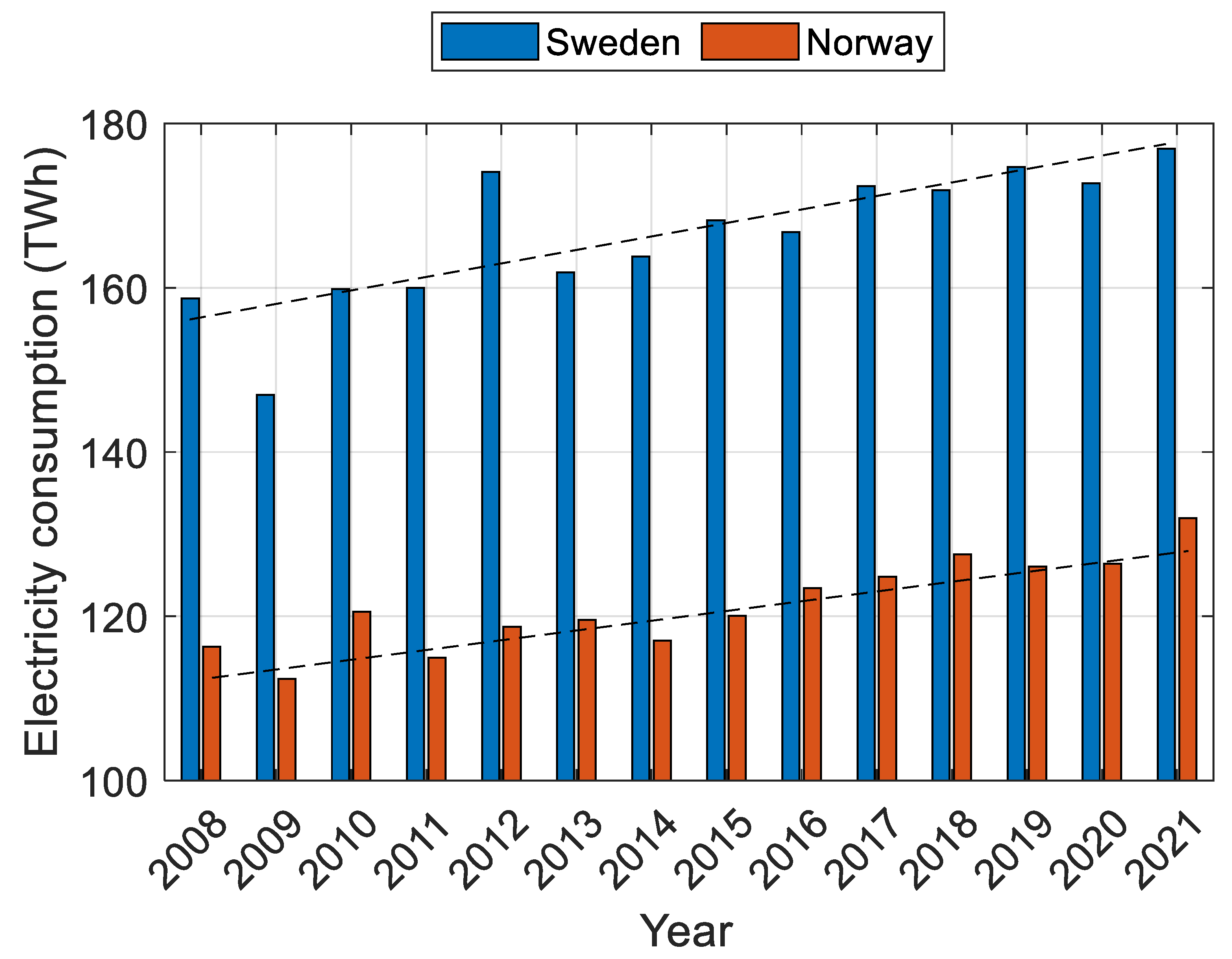
The annual electricity consumption per person in Nordic countries, especially in Sweden, is one of the highest in the world [77]. In Sweden, the residential and service sector uses the most electricity, followed by the industrial sector and the transport sector [71]. According to public data available in [78,79], electricity consumption in both countries has been increasing in recent years, as shown in Figure 18, where the average trend is 1.64 TWh/Year for Sweden and 1.19 TWh/Year for Norway. Considering this increasing trend in electricity consumption, it can be seen that the local maxima for Norway are around 2010, 2018, and 2021, which are in concert with the local minima of the yearly winter temperatures, as seen in Figure 7c,d.
Norway faces an energy deficit almost annually, with the winter season being particularly crucial. This is due to the predominant use of electric heaters in most residential buildings, increased demand from the industrial sector, and the growing need for charging electric cars [74]. Almost 20% of heating comes from electricity [80,81]; consequently, colder winters will directly increase electricity consumption, mainly because people will spend more time at home. Therefore, energy savings should be prioritized in the retrofitting of buildings, even though the investments may not be profitable, as concluded for studied Swedish cities [82]. One promising technology that can be used for multi-family houses is a PV/thermal system combined with a ground-source heat pump system [83]. Energy efficiency should also be increased through the integrated electricity and heating sectors of municipal energy systems, as proposed in [84] for a case study of Piteå in northern Sweden. Another possible source of the increased electricity consumption could be the hydrogen-based steelmaking technology, also known as HYBRIT [85]. In Sweden, HYBRIT requires approximately 10% of electricity generation, which is possible only when electricity exports are reduced [86]. Fortunately, hydrogen storage has the potential to provide balancing services to the power grid.

5.3. Colder Winters, More Likely Storms, and Security of Electricity Supply

As discussed in the previous sections, colder winters in Norway and Sweden generally increase energy consumption and decrease energy generation. In Norway, the electrical energy balance in the winter of 2002/2003 was especially critical due to the limited transmission capacity of power lines between the neighboring regions [74]. The security of electricity supply in Norway was also in focus in the winters of 2009/2010 and 2010/2011 (the years in which AMOC and NAO showed local minima values); however, high prices encouraged lower consumption, higher production, and increased imports of electricity [69]. In Sweden, cold winter events already require an increase in the balancing capacity of the power system, which is needed due to the intermittent generation of wind and solar power units [87,88]. Thus, future research must address the critical question of investments in new storage capacities and equipment for increasing and controlling electrical energy exchange between neighboring regions. Another consideration that might impact the power system operation regarding stability is the amount of inertial energy. From 2017 to 2020, the total inertial energy in Nordic countries decreased by almost 10% [89]. However, the amount of total inertial energy is higher in winter, while the inertial energy of hydropower even started to increase in 2019. Nevertheless, the increased investments in wind power units and the possible shutdown of nuclear power units in Sweden might also reduce the total inertial energy in winter.
More intense winters could result in more storms battering Europe. This, with a weak scenario, could be a further consequence of AMOC weakening [59]. While there may be limited scientific research on this specific aspect, some ecosystem scientists have mentioned it, as reported in sources such as the Guardian [90] or the ClearIAS [91] websites. A study conducted by [92] further supports the notion of increasing storms during the negative phase of the NAO. The major event in Nordic countries was the 2005 Gudrun storm (the year that one of the NAO declines appeared, as reported in Figure 17), causing economic damage to the electric power service, calculated to be around EUR 3 billion [77]. With important evidence, another winter storm in 2011 (the year that AMOC and NAO declines appeared) caused significant disruption in Norway because the high winds brought trees down on power lines [69]. Furthermore, researchers in [93] showed for 30 cities in Sweden that uncertainties in renewable energy potential and demand could lead to a drop in power supply reliability (up to 16%) due to extreme weather events. Such extreme weather events inevitably result in the operation of protection relays to disconnect the faulty elements (power lines, power transformers, and generation units). In order to enhance the resilience of the power grid [94], several measures should be considered, such as the implementation of wide-area monitoring systems in the transmission grid [95,96,97,98,99], smart and closed-loop operation of the distribution grid [100,101,102,103,104,105], as well as the installation of power quality monitoring and mitigation systems in order to check the impact on disturbances such as RMS voltages (daily or in short time intervals) [106,107].

6. Conclusions

This study aimed to investigate the winter temperatures in Norway and northern Sweden over a period ranging from 50 to 71 years. Six locations were selected, including two in Sweden (1 and 2) and four in Norway (3 to 6). The analysis utilized the SSA algorithm to examine the temperature’s long-term trends. The overall long-term trend indicated an increase, which could be attributed to global warming. However, when considering different combinations of highest, lowest, and average temperatures for December, January, and February, 50% of the variations showed a significant decrease in recent years. The average rate of decreasing temperatures was observed as: 0.09, 0.04, 0.088, 0.059, and 0.076 °C/year for locations 2 to 6, respectively, in which locations 2, 4, and 6 experienced colder temperatures, particularly in December, in recent years. The time series of AMOC, a significant climate index, was analyzed from 2004 through to 2020, and the results showed that the values were rarely negative, implying a net flow southward. A maximum positive correlation was observed between AMOC and the Ekman component, showing a direct impact of this component on the AMOC transports. The long-term trend of AMOC measurements presented a 7% general decrease over 17 years, which would lead to an approximate 20% decrease/slowdown forecasted over the first half of the 21st century. However, more data on AMOC would result in more precise results for the AMOC long-term trend concluded from the SSA algorithm. Calculating yearly average values of AMOC transfer variations and its components also showed an anomaly (local minima) during 2009–2010 for all, in 2014 for GS, and in 2019 for both GS and AMOC.
Secondly, the potential similarity between winter AMOC variations and winter temperatures in the six selected locations at mid to high latitudes was investigated. This analysis involved examining the yearly average of winter AMOC and temperatures as well as calculating the lagged correlations between them. The results revealed (1) The possible contribution of AMOC (indirect most likely) to colder winters was realized, particularly around 2010, and further, due to the positive lagged correlations between AMOC and winter temperatures. (2) Higher correlations between winter AMOC and December temperatures (>0.49) were observed specifically in December, for locations 3, 4, and 6. Moreover, higher correlation values were observed for locations 3, 4, and 6. (3) There was a clear pattern where the correlation value increases and the corresponding lag decreases from location 3 to 4 and then to 6, which are those areas along the southern part of the coastline of Norway.
Thirdly, the potential link between another significant climate factor, the NAO, and winter temperatures across the six selected locations was investigated. Similar to the AMOC-temperature analysis, we conducted the same analysis to assess the relationship between the winter NAO index and temperatures, and the results yielded that (1) There is a strong association between the winter NAO and temperatures, specifically in December, for locations 2, 4, 5, and 6, which are situated closer to the coastal areas of Norway but not the northernmost regions. The correlation values between the winter NAO index and December temperatures exceed 0.6, indicating a possible significant influence of NAO on these locations. (2) Among locations 2, 4, 5, and 6, there is a higher probability of experiencing colder winters impacted by the NAO for locations 2, 4, and 5. This conclusion is supported by the following observations: (i) correlation values between the winter NAO index and winter temperatures surpass 0.42; (ii) the highest average rates of temperature decrease were observed earlier for locations 2, 4, and 6.
Fourthly, we examined the impact of colder winters on various aspects of electrical power and energy systems such as electricity generation, electricity consumption, and the security of supply in Sweden and Norway. It was concluded that (1) Colder winters have the potential to reduce reservoir capacities in Norway due to the possibility of ice formation in hydropower units. (2) Reduced electricity generation in Sweden’s winters could shut down the nuclear power units. (3) A possible reduction in electricity generation in Norway and Sweden will also impact the neighboring countries. (4) Colder winters directly increase electricity consumption as the demand for electrical heaters in residual buildings rises. Additionally, increased demand is observed in the industrial sector and for charging electric vehicles. (5) A notable example is the winter of 2010, during which a decline in AMOC, NAO, and winter temperatures coincided with increased electricity consumption in Norway. (6) Winter storms, particularly in colder winters, can pose challenges to the resilience and security of power grids, potentially leading to disruptions in the supply of electricity.
In general, our study reveals several important findings. The cities located near the borders of Norway exhibit an overall upward temperature trend that can be followed with a downward trend. Although there was a moderate correlation, specifically for December, between AMOC and temperatures, there has not been clear evidence of a direct impact of AMOC on the winter temperatures on daily/monthly timescales. Considering the NAO variations, in detail, highlighted that the temperatures in December can be impacted directly from NAO, attached with stronger lagged correlations, albeit to varying degrees across different sites. While we did not specifically examine the AMOC-NAO connection in this study, based on the existing literature it might be concluded that NAO could impact both winter temperatures and AMOC. Understanding the interplay between these climate factors is crucial for comprehending temperature variations. To explain the reasons behind the observed downward temperature trends in most locations and subsequent colder winters in recent years, a detailed investigation is needed. The investigation must consider the maps of the temperature changes and analysis to support the links between the reasons and downward temperatures, and explanations as to why it affects particularly December and some locations differently. While there are many potential reasons for these downtrend trends, some possible scenarios could be the weakening of the climatic indices investigated in this study. Colder winters in Norway and Sweden, whether influenced by AMOC, NAO, or other factors, pose challenges for electrical power and energy systems. Researchers must address the challenges of balancing between generation and consumption as well as ensuring the resilience of power grids, which might be crucial in winter, and it is not a good idea to wait and experience such cold winters unprepared. Finally, it is important to note that the climatic indices of AMOC/NAO are complex and variable systems, and there is still considerable uncertainty surrounding their extent, so further research should focus on improving our understanding of these climate phenomena and their possible role in winter climate patterns. We recommend that future studies employ more robust and physically based methods to estimate the colder winters and the phenomena impacting them, moving beyond the statistical/signal processing approaches used in this study. In particular, it would be beneficial to investigate the influence of winter winds in greater detail across the study locations. Additionally, incorporating another Atlantic index, i.e., Atlantic multidecadal variability (AMV), could provide valuable insights. Expanding the analysis to include more locations across Sweden and Norway, and creating a comprehensive correlation–location map would also enhance our understanding of regional variations.

Author Contributions

Conceptualization, Y.M.; methodology, Y.M.; software, Y.M.; validation, Y.M., A.P., B.P., S.M.M. and D.K.; formal analysis, Y.M. and A.P.; investigation, Y.M., A.P., B.P., S.M.M. and D.K.; resources, Y.M.; data curation, Y.M.; writing—original draft preparation, Y.M.; writing—review and editing, Y.M., A.P., B.P., S.M.M. and D.K.; visualization, Y.M., A.P., B.P., S.M.M. and D.K.; supervision, D.K.; project administration, D.K. All authors have read and agreed to the published version of the manuscript.

Funding

This research was funded by the Kempe Foundation (Kempestiftelserna) (https://www.kempe.com/), grant (funding) number JCK22-0025. Data from the RAPID AMOC monitoring project are also funded by the Natural Environment Research Council.

Data Availability Statement

Data regarding the temperature at the selected locations are freely available from https://seklima.met.no/observations, accessed on 1 February 2023 and https://www.smhi.se/en/theme/climate-centre. Data from the RAPID AMOC monitoring are also freely accessible from www.rapid.ac.uk/rapidmoc, accessed on 26 January 2023. The website https://ftp.cpc.ncep.noaa.gov/cwlinks/ provides free access to the daily NAO index monitoring data, accessed on 15 May 2023.

Conflicts of Interest

The authors declare no conflict of interest. The funders had no role in the design of the study; in the collection, analyses, or interpretation of data; in the writing of the manuscript; or in the decision to publish the results.

Appendix A

Figure A1 gives the correlation coefficient and corresponding p-values using Kendal and Spearman methods.
Figure A1. Coefficient correlations and corresponding p-values: (a,c) Kendal; (b,d) Spearman.
Energies 16 05575 g0a1
Figure A2 shows an uncompressed version of the temperature plotted in Figure 10a to give an understanding of smoothed jumps between each month over different years.
Figure A2. An uncompressed version of the temperature plotted in Figure 10a.
Energies 16 05575 g0a2

References

  1. O’Hare, G. Updating Our Understanding of Climate Change in the North Atlantic: The Role of Global Warming and the Gulf Stream. Geography 2011, 96, 5–15. [Google Scholar] [CrossRef]
  2. Lozier, M.S. Overturning in the North Atlantic. Ann. Rev. Mar. Sci. 2011, 4, 291–315. [Google Scholar] [CrossRef] [Green Version]
  3. Willis, J.K. Can in Situ Floats and Satellite Altimeters Detect Long-Term Changes in Atlantic Ocean Overturning? Geophys. Res. Lett. 2010, 37. [Google Scholar] [CrossRef] [Green Version]
  4. Xu, X.; Chassignet, E.P.; Johns, W.E.; Schmitz, W.J.; Metzger, E.J. Intraseasonal to Interannual Variability of the Atlantic Meridional Overturning Circulation from Eddy-Resolving Simulations and Observations. J. Geophys. Res. 2014, 119, 5140–5159. [Google Scholar] [CrossRef]
  5. Johns, W.E.; Baringer, M.O.; Beal, L.M.; Cunningham, S.A.; Kanzow, T.; Bryden, H.L.; Hirschi, J.J.M.; Marotzke, J.; Meinen, C.S.; Shaw, B.; et al. Continuous, Array-Based Estimates of Atlantic Ocean Heat Transport at 26.5° N. J. Clim. 2011, 24, 2429–2449. [Google Scholar] [CrossRef] [Green Version]
  6. McDonagh, E.L.; King, B.A.; Bryden, H.L.; Courtois, P.; Szuts, Z.; Baringer, M.; Cunningham, S.A.; Atkinson, C.; McCarthy, G. Continuous Estimate of Atlantic Oceanic Freshwater Flux at 26.5° N. J. Clim. 2015, 28, 8888–8906. [Google Scholar] [CrossRef]
  7. Talley, L.D.; Feely, R.A.; Sloyan, B.M.; Wanninkhof, R.; Baringer, M.O.; Bullister, J.L.; Carlson, C.A.; Doney, S.C.; Fine, R.A.; Firing, E.; et al. Changes in Ocean Heat, Carbon Content, and Ventilation: A Review of the First Decade of GO-SHIP Global Repeat Hydrography. Ann. Rev. Mar. Sci. 2016, 8, 185–215. [Google Scholar] [CrossRef] [Green Version]
  8. Seidov, D.; Mishonov, A.; Reagan, J.; Parsons, R. Multidecadal Variability and Climate Shift in the North Atlantic Ocean. Geophys. Res. Lett. 2017, 44, 4985–4993. [Google Scholar] [CrossRef]
  9. Lavoie, D.; Lambert, N.; Gilbert, D. Projections of Future Trends in Biogeochemical Conditions in the Northwest Atlantic Using CMIP5 Earth System Models. Atmosphere-Ocean 2019, 57, 18–40. [Google Scholar] [CrossRef] [Green Version]
  10. Portis, D.H.; Walsh, J.E.; El Hamly, M.; Lamb, P.J. Seasonality of the North Atlantic Oscillation. J. Clim. 2001, 14, 2069–2078. [Google Scholar] [CrossRef]
  11. Yang, H.; Lohmann, G.; Wei, W.; Dima, M.; Ionita, M.; Liu, J. Intensification and Poleward Shift of Subtropical Western Boundary Currents in a Warming Climate. J. Geophys. Res. Ocean. 2016, 121, 4928–4945. [Google Scholar] [CrossRef] [Green Version]
  12. Delworth, T.L.; Zeng, F. The Impact of the North Atlantic Oscillation on Climate through Its Influence on the Atlantic Meridional Overturning Circulation. J. Clim. 2016, 29, 941–962. [Google Scholar] [CrossRef]
  13. Li, M.; Yao, Y.; Simmonds, I.; Luo, D.; Zhong, L.; Chen, X. Collaborative Impact of the Nao and Atmospheric Blocking on European Heatwaves, with a Focus on the Hot Summer of 2018. Environ. Res. Lett. 2020, 15, 114003. [Google Scholar] [CrossRef]
  14. Buckley, M.W.; Marshall, J. Observations, Inferences, and Mechanisms of the Atlantic Meridional Overturning Circulation: A Review. Rev. Geophys. 2016, 54, 5–63. [Google Scholar] [CrossRef] [Green Version]
  15. Rahmstorf, S.; Box, J.E.; Feulner, G.; Mann, M.E.; Robinson, A.; Rutherford, S.; Schaffernicht, E.J. Exceptional Twentieth-Century Slowdown in Atlantic Ocean Overturning Circulation. Nat. Clim. Chang. 2015, 5, 475–480. [Google Scholar] [CrossRef] [Green Version]
  16. Smeed, D.A.; McCarthy, G.D.; Cunningham, S.A.; Frajka-Williams, E.; Rayner, D.; Johns, W.E.; Meinen, C.S.; Baringer, M.O.; Moat, B.I.; Duchez, A.; et al. Observed Decline of the Atlantic Meridional Overturning Circulation 2004–2012. Ocean Sci. 2014, 10, 29–38. [Google Scholar] [CrossRef] [Green Version]
  17. IPCC. CLIMATE CHANGE 2013 Climate Change 2013; IPCC: Geneva, Switzerland, 2013; ISBN 9781107661820. [Google Scholar]
  18. Longworth, H.R.; Bryden, H.L.; Baringer, M.O. Historical Variability in Atlantic Meridional Baroclinic Transport at 26.5° N from Boundary Dynamic Height Observations. Deep. Res. Part II Top. Stud. Oceanogr. 2011, 58, 1754–1767. [Google Scholar] [CrossRef]
  19. Bryden, H.L.; Longworth, H.R.; Cunningham, S.A. Slowing of the Atlantic Meridional Overturning Circulation at 25 Degrees N. Nature 2005, 438, 655–657. [Google Scholar] [CrossRef]
  20. Kanzow, T.; Cunningham, S.A.; Johns, W.E.; Hirschi, J.J.M.; Marotzke, J.; Baringer, M.O.; Meinen, C.S.; Chidichimo, M.P.; Atkinson, C.; Beal, L.M.; et al. Seasonal Variability of the Atlantic Meridional Overturning Circulation at 26.5° N. J. Clim. 2010, 23, 5678–5698. [Google Scholar] [CrossRef] [Green Version]
  21. Jewett, L.; Romanou, A. Ocean acidification and other ocean changes. In Climate Science Special Report: Fourth National Climate Assessment; Wuebbles, D.J., Fahey, D.W., Hibbard, K.A., Dokken, D.J., Stewart, B.C., Maycock, T.K., Eds.; U.S. Global Change Research Program: Washington, DC, USA, 2017; Volume I, pp. 364–392. [Google Scholar] [CrossRef] [Green Version]
  22. Weijer, W.; Cheng, W.; Garuba, O.A.; Hu, A.; Nadiga, B.T. CMIP6 Models Predict Significant 21st Century Decline of the Atlantic Meridional Overturning Circulation. Geophys. Res. Lett. 2020, 47, e2019GL086075. [Google Scholar] [CrossRef]
  23. Zhang, W.-Z.; Chai, F.; Xue, H.; Oey, L.-Y. Remote Sensing Linear Trends of the Gulf Stream from 1993 to 2016. Ocean Dyn. 2020, 70. [Google Scholar] [CrossRef]
  24. Andres, M.; Donohue, K.A.; Toole, J.M. The Gulf Stream’s Path and Time-Averaged Velocity Structure and Transport at 68.5° W and 70.3° W. Deep Sea Res. Part I Oceanogr. Res. Pap. 2020, 156, 103179. [Google Scholar] [CrossRef]
  25. Fox-Kemper, B. Ocean, Cryosphere and Sea Level Change. In Proceedings of the AGU Fall Meeting Abstracts, New Orleans, LA, USA, 13–17 December 2021; Volume 2021, p. U13B-09. [Google Scholar]
  26. Yang, H.; Chen, G.; Tang, Q.; Hess, P. Quantifying Isentropic Stratosphere-Troposphere Exchange of Ozone. J. Geophys. Res. Atmos. 2016, 121, 3372–3387. [Google Scholar] [CrossRef] [Green Version]
  27. Chen, C.; Wang, G.; Xie, S.-P.; Liu, W. Why Does Global Warming Weaken the Gulf Stream but Intensify the Kuroshio? J. Clim. 2019, 32, 7437–7451. [Google Scholar] [CrossRef]
  28. Caesar, L.; Rahmstorf, S.; Robinson, A.G.; Feulner, G.; Saba, V.S. Observed Fingerprint of a Weakening Atlantic Ocean Overturning Circulation. Nature 2017, 556, 191–196. [Google Scholar] [CrossRef] [PubMed]
  29. Ortega, P.; Robson, J.; Sutton, R.; Andrews, M. Mechanisms of Decadal Variability in the Labrador Sea and the Wider North Atlantic in a High-Resolution Climate Model. Clim. Dyn. 2017, 49, 2625–2647. [Google Scholar] [CrossRef] [Green Version]
  30. Belonenko, T.; Morozova, L.; Gordeeva, S. Key to the Atlantic Gates of the Arctic. Russ. J. Earth Sci. 2022, 22, 2004. [Google Scholar] [CrossRef]
  31. Caesar, L.; McCarthy, G.; Thornalley, D.; Cahill, N.; Rahmstorf, S. Current Atlantic Meridional Overturning Circulation Weakest in Last Millennium. Nat. Geosci. 2021, 14, 1–3. [Google Scholar] [CrossRef]
  32. Biastoch, A.; Schwarzkopf, F.U.; Getzlaff, K.; Rühs, S.; Martin, T.; Scheinert, M.; Schulzki, T.; Handmann, P.; Hummels, R.; Böning, C.W. Regional Imprints of Changes in the Atlantic Meridional Overturning Circulation in the Eddy-Rich Ocean Model VIKING20X. Ocean Sci. 2021, 17, 1177–1211. [Google Scholar] [CrossRef]
  33. University of South Florida (USF Innovation). Melting Greenland ice Sheet may Affect Global Ocean Circulation, Future Climate: University of South Florida and International Scientists Find Influx of Freshwater Could Disrupt the Atlantic Meridional Overturning Circulation, an Important Component of Global Ocean Circulation. ScienceDaily, 22 January 2016. Available online: www.sciencedaily.com/releases/2016/01/160122122629.htm (accessed on 24 February 2023).
  34. Ciemer, C.; Winkelmann, R.; Kurths, J.; Boers, N. Impact of an AMOC Weakening on the Stability of the Southern Amazon Rainforest. Eur. Phys. J. Spec. Top. 2021, 230, 3065–3073. [Google Scholar] [CrossRef]
  35. Liu, W.; Fedorov, A.V.; Xie, S.-P.; Hu, S. Climate Impacts of a Weakened Atlantic Meridional Overturning Circulation in a Warming Climate. Sci. Adv. 2020, 6, eaaz4876. [Google Scholar] [CrossRef]
  36. Wang, H.; Zuo, Z.; Qiao, L.; Zhang, K.; Sun, C.; Xiao, D.; Bu, L. Frequency of Winter Temperature Extremes over Northern Eurasia Dominated by AMOC. npj Clim. Atmos. Sci. 2021, 5, 84. [Google Scholar] [CrossRef]
  37. Smeed, D.; Wood, R.; Cunningham, S.; Mccarthy, G.; Kuhlbrodt, T.; Office, M.; Centre, H. Impacts of Climate Change on the Atlantic Heat Conveyor. MCCP Sci. Rev. 2013, 4, 49–59. [Google Scholar] [CrossRef]
  38. Buchan, J.; Hirschi, J.J.M.; Blaker, A.T.; Sinha, B. North Atlantic SST Anomalies and the Cold North European Weather Events of Winter 2009/10 and December 2010. Mon. Weather Rev. 2014, 142, 922–932. [Google Scholar] [CrossRef] [Green Version]
  39. Bryden, H.L.; King, B.A.; McCarthy, G.D.; McDonagh, E.L. Impact of a 30% Reduction in Atlantic Meridional Overturning during 2009–2010. Ocean Sci. 2014, 10, 683–691. [Google Scholar] [CrossRef] [Green Version]
  40. Munday, A.J.; Hunt, J.B. University of Southampton. Tribology 1970, 3, 106–107. [Google Scholar] [CrossRef]
  41. Bellomo, K.; Meccia, V.; D’Agostino, R.; Fabiano, F.; von Hardenberg, J.; Corti, S. The Climate Impacts of an Abrupt AMOC Weakening on the European Winters. In Proceedings of the EGU General Assembly 2022, Vienna, Austria, 23–27 May 2022. EGU22-1023. [Google Scholar] [CrossRef]
  42. RAPID: Monitoring the Atlantic Meridional Overturning Circulation at 26.5 N since 2004. Available online: https://rapid.ac.uk/rapidmoc/overview.php (accessed on 26 January 2023).
  43. Duchez, A.; Courtois, P.; Harris, E.; Josey, S.A.; Kanzow, T.; Marsh, R.; Smeed, D.A.; Hirschi, J.J.M. Potential for Seasonal Prediction of Atlantic Sea Surface Temperatures Using the RAPID Array at 26° N. Clim. Dyn. 2016, 46, 3351–3370. [Google Scholar] [CrossRef] [Green Version]
  44. Moat, B.I.; Smeed, D.A.; Frajka-Williams, E.; Desbruyères, D.G.; Beaulieu, C.; Johns, W.E.; Rayner, D.; Sanchez-Franks, A.; Baringer, M.O.; Volkov, D.; et al. Pending Recovery in the Strength of the Meridional Overturning Circulation at 26° N. Ocean Sci. 2020, 16, 863–874. [Google Scholar] [CrossRef]
  45. Wanner, H.; Brönnimann, S.; Casty, C.; Gyalistras, D.; Luterbacher, J.; Schmutz, C.; Stephenson, D.B.; Xoplaki, E. North Atlantic Oscillation–Concepts And Studies. Surv. Geophys. 2001, 22, 321–381. [Google Scholar] [CrossRef]
  46. Stephenson, D.B.; Wanner, H.; Brönnimann, S.; Luterbacher, J. The History of Scientific Research on the North Atlantic Oscillation. In The North Atlantic Oscillation: Climatic Significance and Environmental Impact; American Geophysical Union (AGU): Washington, DC, USA, 2003; pp. 37–50. ISBN 9781118669037. [Google Scholar]
  47. Norsk Klimaservicesenter. Available online: https://seklima.met.no/observations (accessed on 26 January 2023).
  48. Swedish National Knowledge Centre for Climate Change Adaptation|SMHI. Available online: https://www.smhi.se/en/theme/climate-centre (accessed on 26 January 2023).
  49. Monitoring North Atlantic Oscillation Since 1950. Available online: Https://Ftp.Cpc.Ncep.Noaa.Gov/Cwlinks/ (accessed on 15 May 2023).
  50. Sinha, B.; Smeed, D.A.; McCarthy, G.; Moat, B.I.; Josey, S.A.; Hirschi, J.J.-M.; Frajka-Williams, E.; Blaker, A.T.; Rayner, D.; Madec, G. The Accuracy of Estimates of the Overturning Circulation from Basin-Wide Mooring Arrays. Prog. Oceanogr. 2018, 160, 101–123. [Google Scholar] [CrossRef]
  51. McCarthy, G.D.; Brown, P.J.; Flagg, C.N.; Goni, G.; Houpert, L.; Hughes, C.W.; Hummels, R.; Inall, M.; Jochumsen, K.; Larsen, K.M.H.; et al. Sustainable Observations of the AMOC: Methodology and Technology. Rev. Geophys. 2020, 58, e2019RG000654. [Google Scholar] [CrossRef] [Green Version]
  52. Boschat, G.; Simmonds, I.; Purich, A.; Cowan, T.; Pezza, A.B. On the Use of Composite Analyses to Form Physical Hypotheses: An Example from Heat Wave-SST Associations. Sci. Rep. 2016, 6, 29599. [Google Scholar] [CrossRef] [PubMed] [Green Version]
  53. Deng, C. Time Series Decomposition Using Singular Spectrum Analysis Part of the Longitudinal Data Analysis and Time Series Commons. Master’s Thesis, East Tennessee State University, Johnson City, TN, USA, 2014. [Google Scholar]
  54. Golyandina, N. Particularities and Commonalities of Singular Spectrum Analysis as a Method of Time Series Analysis and Signal Processing. WIREs Comput. Stat. 2020, 12, e1487. [Google Scholar] [CrossRef]
  55. Miraftabzadeh, S.M.; Longo, M.; Brenna, M.; Pasetti, M. Data-Driven Model for PV Power Generation Patterns Extraction via Unsupervised Machine Learning Methods. In Proceedings of the 2022 North American Power Symposium (NAPS), Salt Lake City, UT, USA, 9–11 October 2022; pp. 1–5. [Google Scholar]
  56. Miraftabzadeh, S.M.; Longo, M.; Brenna, M. Knowledge Extraction from PV Power Generation with Deep Learning Autoencoder and Clustering-Based Algorithms. IEEE Access 2023, 11, 69227–69240. [Google Scholar] [CrossRef]
  57. Li, H. Spectral Analysis of Signals [Book Review]; IEEE: Piscataway, NJ, USA, 2008; Volume 24, ISBN 0131139568. [Google Scholar]
  58. Muir, L.C.; Fedorov, A.V. How the AMOC Affects Ocean Temperatures on Decadal to Centennial Timescales: The North Atlantic versus an Interhemispheric Seesaw. Clim. Dyn. 2015, 45, 151–160. [Google Scholar] [CrossRef]
  59. Bellomo, K.; Agostino, R.D.; Fabiano, F.; Larson, S.M.; Corti, S. Impacts of a Weakened AMOC on Precipitation over the Euro- Atlantic Region in the EC-Earth3 Climate Model. Clim. Dyn. 2022. [Google Scholar] [CrossRef]
  60. Chiang, J.C.H.; Cheng, W.; Kim, W.M.; Kim, S. Untangling the Relationship Between AMOC Variability and North Atlantic Upper-Ocean Temperature and Salinity. Geophys. Res. Lett. 2021, 48, e2021GL093496. [Google Scholar] [CrossRef]
  61. López-Moreno, J.I.; Vicente-Serrano, S.M.; Morán-Tejeda, E.; Lorenzo-Lacruz, J.; Kenawy, A.; Beniston, M. Effects of the North Atlantic Oscillation (NAO) on Combined Temperature and Precipitation Winter Modes in the Mediterranean Mountains: Observed Relationships and Projections for the 21st Century. Glob. Planet. Chang. 2011, 77, 62–76. [Google Scholar] [CrossRef]
  62. Rousi, E.; Rust, H.W.; Ulbrich, U.; Anagnostopoulou, C. Implications of Winter NAO Flavors on Present and Future European Climate. Climate 2020, 8, 13. [Google Scholar] [CrossRef] [Green Version]
  63. Jackson, L.C.; Biastoch, A.; Buckley, M.W.; Desbruyères, D.G.; Frajka-Williams, E.; Moat, B.; Robson, J. The Evolution of the North Atlantic Meridional Overturning Circulation since 1980. Nat. Rev. Earth Environ. 2022, 3, 241–254. [Google Scholar] [CrossRef]
  64. Roach, L.A.; Blanchard-Wrigglesworth, E.; Ragen, S.; Cheng, W.; Armour, K.C.; Bitz, C.M. The Impact of Winds on AMOC in a Fully-Coupled Climate Model. Geophys. Res. Lett. 2022, 49, 1–10. [Google Scholar] [CrossRef]
  65. Kim, H.J.; An, S.I.; Park, J.H.; Sung, M.K.; Kim, D.; Choi, Y.; Kim, J.S. North Atlantic Oscillation Impact on the Atlantic Meridional Overturning Circulation Shaped by the Mean State. npj Clim. Atmos. Sci. 2023, 6. [Google Scholar] [CrossRef]
  66. Iversen, E.C.; Burningham, H. Relationship between NAO and Wind Climate over Norway. Clim. Res. 2015, 63, 115–134. [Google Scholar] [CrossRef]
  67. Xu, Y. Estimates of Changes in Surface Wind and Temperature Extremes in Southwestern Norway Using Dynamical Downscaling Method under Future Climate. Weather Clim. Extrem. 2019, 26, 100234. [Google Scholar] [CrossRef]
  68. ENTSO-E Transparency Platform. Available online: https://transparency.entsoe.eu/ (accessed on 24 February 2023).
  69. Energifaktanorge.No-Fakta Om Norsk Energi Og Vannressurser-Energifakta Norge. Available online: https://energifaktanorge.no/ (accessed on 24 February 2023).
  70. An Overview of Energy in Sweden 2022 Now Available. Available online: https://www.energimyndigheten.se/en/news/2022/an-overview-of-energy-in-sweden-2022-now-available/ (accessed on 24 February 2023).
  71. Quarterly Statistics-Swedish Wind Energy Association. Available online: https://swedishwindenergy.com/statistics (accessed on 24 February 2023).
  72. Haddeland, I.; Hole, J.; Holmqvist, E.; Koestler, V.; Sidelnikova, M.; Veie, C.A.; Wold, M. Effects of Climate on Renewable Energy Sources and Electricity Supply in Norway. Renew. Energy 2022, 196, 625–637. [Google Scholar] [CrossRef]
  73. Heggenes, J.; Stickler, M.; Alfredsen, K.; Brittain, J.E.; Adeva-Bustos, A.; Huusko, A. Hydropower-Driven Thermal Changes, Biological Responses and Mitigating Measures in Northern River Systems. River Res. Appl. 2021, 37, 743–765. [Google Scholar] [CrossRef]
  74. François, B.; Martino, S.; Tøfte, L.S.; Hingray, B.; Mo, B.; Creutin, J.-D. Effects of Increased Wind Power Generation on Mid-Norway’s Energy Balance under Climate Change: A Market Based Approach. Energies 2017, 10, 227. [Google Scholar] [CrossRef] [Green Version]
  75. Farsaei, A.; Syri, S.; Olkkonen, V.; Khosravi, A. Unintended Consequences of National Climate Policy on International Electricity Markets—Case Finland’s Ban on Coal-Fired Generation. Energies 2020, 13, 1930. [Google Scholar] [CrossRef] [Green Version]
  76. Olkkonen, V.; Syri, S. Spatial and Temporal Variations of Marginal Electricity Generation: The Case of the Finnish, Nordic, and European Energy Systems up to 2030. J. Clean. Prod. 2016, 126, 515–525. [Google Scholar] [CrossRef]
  77. Gündüz, N.; Küfeoğlu, S.; Lehtonen, M. Impacts of Natural Disasters on Swedish Electric Power Policy: A Case Study. Sustainability 2017, 9, 230. [Google Scholar] [CrossRef] [Green Version]
  78. Available online: https://www.statista.com/Statistics/1027078/Electricity-Consumption-in-Sweden/ (accessed on 5 May 2023).
  79. Available online: https://www.statista.com/Statistics/1024933/Net-Consumption-of-Electricity-in-Norway/ (accessed on 25 January 2023).
  80. Energimyndigheten. Available online: https://www.energimyndigheten.se/ (accessed on 26 January 2023).
  81. Renewable Energy Production in Norway. Available online: https://www.regjeringen.no/en/topics/energy/renewable-energy/renewable-energy-production-in-norway/id2343462/ (accessed on 11 May 2016).
  82. Mata, É.; Wanemark, J.; Nik, V.M.; Sasic Kalagasidis, A. Economic Feasibility of Building Retrofitting Mitigation Potentials: Climate Change Uncertainties for Swedish Cities. Appl. Energy 2019, 242, 1022–1035. [Google Scholar] [CrossRef]
  83. Sommerfeldt, N.; Madani, H. In-Depth Techno-Economic Analysis of PV/Thermal plus Ground Source Heat Pump Systems for Multi-Family Houses in a Heating Dominated Climate. Sol. Energy 2019, 190, 44–62. [Google Scholar] [CrossRef]
  84. Fischer, R.; Elfgren, E.; Toffolo, A. Towards Optimal Sustainable Energy Systems in Nordic Municipalities. Energies 2020, 13, 290. [Google Scholar] [CrossRef] [Green Version]
  85. Hybrit. Available online: https://www.hybritdevelopment.se/en/ (accessed on 24 February 2023).
  86. Öhman, A.; Karakaya, E.; Urban, F. Enabling the Transition to a Fossil-Free Steel Sector: The Conditions for Technology Transfer for Hydrogen-Based Steelmaking in Europe. Energy Res. Soc. Sci. 2022, 84, 102384. [Google Scholar] [CrossRef]
  87. Höltinger, S.; Mikovits, C.; Schmidt, J.; Baumgartner, J.; Arheimer, B.; Lindström, G.; Wetterlund, E. The Impact of Climatic Extreme Events on the Feasibility of Fully Renewable Power Systems: A Case Study for Sweden. Energy 2019, 178, 695–713. [Google Scholar] [CrossRef] [Green Version]
  88. Miraftabzadeh, S.M.; Longo, M. High-Resolution PV Power Prediction Model Based on the Deep Learning and Attention Mechanism. Sustain. Energy Grids Networks 2023, 34, 101025. [Google Scholar] [CrossRef]
  89. Graham, J.; Heylen, E.; Bian, Y.; Teng, F. Benchmarking Explanatory Models for Inertia Forecasting Using Public Data of the Nordic Area. In Proceedings of the 2022 17th International Conference on Probabilistic Methods Applied to Power Systems (PMAPS), Lisbon, Portugal, 12–15 June 2022; pp. 1–6. [Google Scholar]
  90. Atlantic Ocean Circulation at Weakest in a Millennium, Say Scientists|Climate Crisis|The Guardian. Available online: https://www.theguardian.com/environment/2021/feb/25/atlantic-ocean-circulation-at-weakest-in-a-millennium-say-scientists (accessed on 26 January 2023).
  91. Available online: https://www.clearias.com/atlantic-meridional-overturning-circulation/ (accessed on 20 December 2022).
  92. Chartrand, J.; Pausata, F.S.R. Impacts of the North Atlantic Oscillation on Winter Precipitations and Storm Track Variability in Southeast Canada and the Northeast United States. Weather Clim. Dyn. 2020, 1, 731–744. [Google Scholar] [CrossRef]
  93. Perera, A.T.D.; Nik, V.M.; Chen, D.; Scartezzini, J.-L.; Hong, T. Quantifying the Impacts of Climate Change and Extreme Climate Events on Energy Systems. Nat. Energy 2020, 5, 150–159. [Google Scholar] [CrossRef] [Green Version]
  94. de Morais, S.G.; Resener, M.; Ramos, J.S.M.; Mohammadi, Y. Estabilidade Transitória de Sistemas de Distribuição Ativos Com Recursos Energéticos Distribuídos: Um Estudo de Caso. Secr. SBA 2020, 2, 1. [Google Scholar] [CrossRef]
  95. Mohammadi, Y.; Moradi, M.H.; Chouhy Leborgne, R. Employing Instantaneous Positive Sequence Symmetrical Components for Voltage Sag Source Relative Location. Electr. Power Syst. Res. 2017, 151, 186–196. [Google Scholar] [CrossRef]
  96. Mohammadi, Y.; Salarpour, A.; Chouhy Leborgne, R. Comprehensive Strategy for Classification of Voltage Sags Source Location Using Optimal Feature Selection Applied to Support Vector Machine and Ensemble Techniques. Int. J. Electr. Power Energy Syst. 2021, 124, 106363. [Google Scholar] [CrossRef]
  97. Shazdeh, S.; Golpîra, H.; Bevrani, H. A PMU-Based Back-up Protection Scheme for Fault Detection Considering Uncertainties. Int. J. Electr. Power Energy Syst. 2023, 145, 108592. [Google Scholar] [CrossRef]
  98. Liu, T.; Tang, Z.; Huang, Y.; Xu, L.; Yang, Y. Online Prediction and Control of Post-Fault Transient Stability Based on PMU Measurements and Multi-Task Learning. Front. Energy Res. 2023, 10, 1084295. [Google Scholar] [CrossRef]
  99. Alqudah, M.; Kezunovic, M.; Obradovic, Z. Automated Power System Fault Prediction and Precursor Discovery Using Multi-Modal Data. IEEE Access 2023, 11, 7283–7296. [Google Scholar] [CrossRef]
  100. Mohammadi, Y.; Leborgne, R.C. A New Approach for Voltage Sag Source Relative Location in Active Distribution Systems with the Presence of Inverter-Based Distributed Generations. Electr. Power Syst. Res. 2020, 182, 106222. [Google Scholar] [CrossRef]
  101. Moradi, M.H.; Mohammadi, Y.; Hoseyni Tayyebi, M. A Novel Method to Locate the Voltage Sag Source: A Case Study in the Brazilian Power Network (Mato Grosso). Prz. Elektrotechniczny 2012, 88, 112–115. [Google Scholar]
  102. Mohammadi, Y.; Leborgne, R.C.; Polajžer, B. Modified Methods for Voltage-Sag Source Detection Using Transient Periods. Electr. Power Syst. Res. 2022, 207, 107857. [Google Scholar] [CrossRef]
  103. Mohammadi, Y.; Miraftabzadeh, S.M.; Bollen, M.H.J.; Longo, M. Voltage-Sag Source Detection: Developing Supervised Methods and Proposing a New Unsupervised Learning. Sustain. Energy, Grids Networks 2022, 32, 100855. [Google Scholar] [CrossRef]
  104. Štumbrger, G.; Rošer, M.; Pintarič, M.; Polajžer, B. Permanent Closed-Loop Operation as a Measure for Improving Power Supply Reliability in a Rural Medium Voltage Distribution Network. Renew. Energy Power Qual. J. 2021, 19, 523–527. [Google Scholar] [CrossRef]
  105. Mohammadi, Y.; Leborgne, R.C. Improved DR and CBM Methods for Finding Relative Location of Voltage Sag Source at the PCC of Distributed Energy Resources. Int. J. Electr. Power Energy Syst. 2020, 117, 105664. [Google Scholar] [CrossRef]
  106. Mohammadi, Y.; Miraftabzadeh, S.M.; Bollen, M.H.J.; Longo, M. An Unsupervised Learning Schema for Seeking Patterns in Rms Voltage Variations at the Sub-10-Minute Time Scale. Sustain. Energy Grids Networks 2022, 31, 100773. [Google Scholar] [CrossRef]
  107. Mohammadi, Y.; Mahdi Miraftabzadeh, S.; Bollen, M.H.J.; Longo, M. Seeking Patterns in Rms Voltage Variations at the Sub-10-Minute Scale from Multiple Locations via Unsupervised Learning and Patterns’ Post-Processing. Int. J. Electr. Power Energy Syst. 2022, 143, 108516. [Google Scholar] [CrossRef]
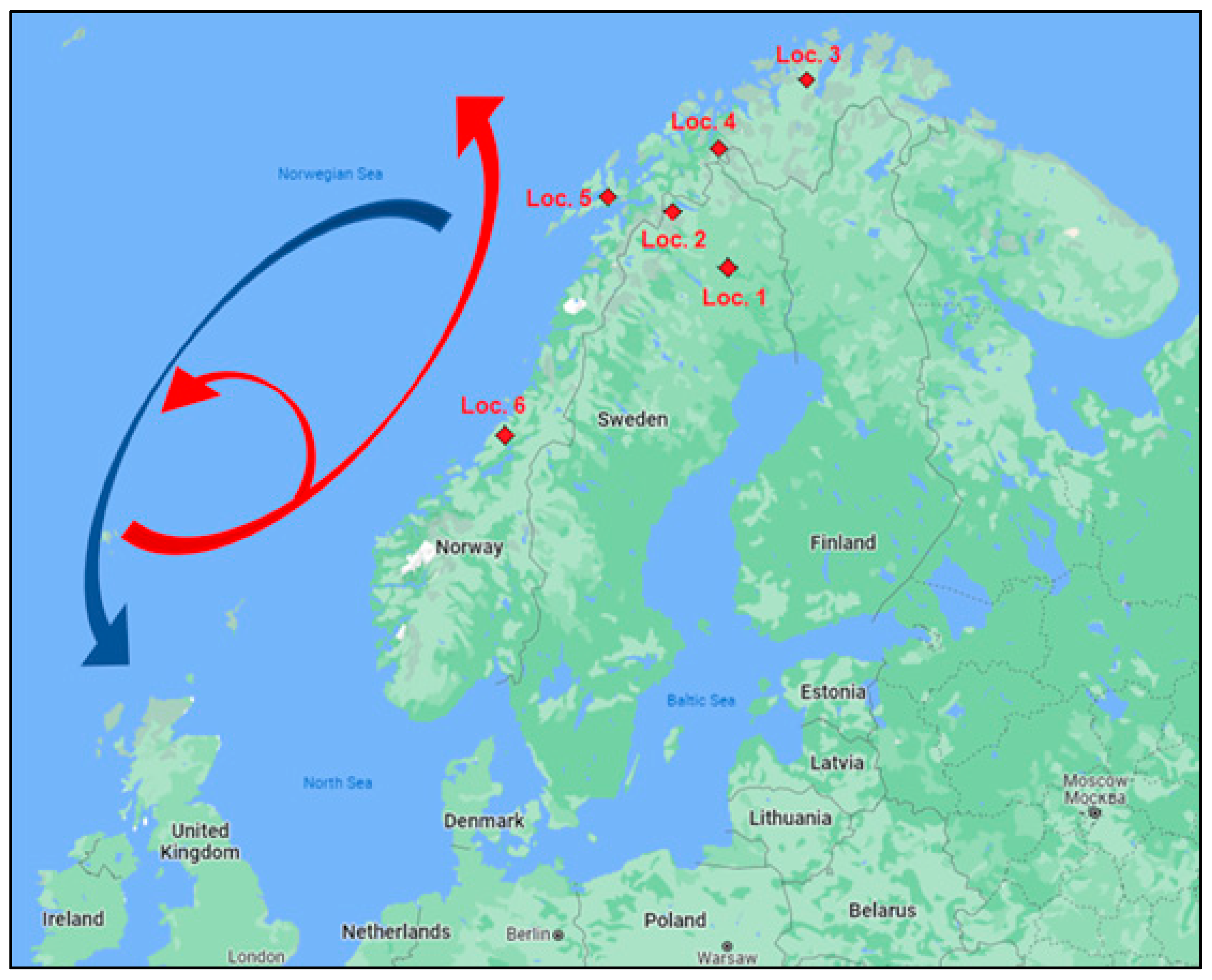
Figure 1. The geographical representation of the six selected locations in Northern Sweden and Norway (Loc. 1 to 6). The part of the northward red arrow (warm surface flow of AMOC) and the southward blue arrow (deep cold flow of AMOC) are marked. However, the real circulation of the arrows is from the Antarctic Ocean to the Greenland Sea and back.
Energies 16 05575 g001
Figure 2. Daily time series of AMOC and its components from 7 April 2004 to 10 December 2020. Positive transports correspond to northward flow, while negative values show southward flow. AMOC negative values are marked by *.
Energies 16 05575 g002
Figure 3. Correlation between daily time series of AMOC and its components: (a) Pearson coefficients; (b) p-values corresponded; (c) Minimum/Maximum Pearson lagged correlation.
Energies 16 05575 g003
Figure 4. Overturning strength of AMOC (Sv): (a) Daily time series; (b) Long-term trend; (c) Oscillation trend; (d) Residual. The dashed vertical lines in (a) show the points of the year at which the mean of transport (red horizontal lines in (a)) changes most significantly.
Energies 16 05575 g004
Figure 5. AMOC components in terms of long and seasonal trends: (a,c,e) Long-term trends for UMO, GS, and Ekman; (b,d,f) Seasonal trends for UMO, GS, and Ekman.
Energies 16 05575 g005
Figure 6. The annual average of AMOC and its components in (Sv): (a) AMOC; (b) UMO; (c) GS; (d) Ekman. OS values are given as mean, + standard deviation, and − standard deviation. Red dashed lines show the standard deviation in (ad).
Energies 16 05575 g006
Figure 7. Yearly winter (December, January, and February) average temperatures for the selected locations 1 to 6 from 2004 to present (af).
Energies 16 05575 g007
Figure 8. The daily highest temperatures (with a 10-day running averaging window) for all winter months in location 1: (a) Time series; (b) Long-term trend. Same legend as used in (b) apply in (a).
Energies 16 05575 g008
Figure 9. The daily highest temperatures (with a 10-day running averaging window) for January and February in location 2: (a,b) Time series; (c,d) Long-term trend. The arrows in (c,d) show the beginning and end of the downward sector in the long-term trend marked by an ellipse.
Energies 16 05575 g009
Figure 10. The daily highest temperatures (with a 10-day running averaging window) for December and January in location 3: (a,b) Time series; (c,d) Long-term trend. The arrows in (c,d) show the beginning and end of the downward sector in the long-term trend marked by an ellipse.
Energies 16 05575 g010
Figure 11. The daily temperatures (with a 10-day running averaging window) in location 4: (a,c) Time series and long-term trend for average temperature in December; (b,d) Time series and long-term trend for highest temperature in February. The arrows in (c,d) show the beginning and end of the downward sector in the long-term trend marked by an ellipse.
Energies 16 05575 g011
Figure 12. The daily highest temperatures (with a 10-day running averaging window) for January and February in location 5: (a,b) Time series; (c,d) Long-term trend. The arrows in (c,d) show the beginning and end of the downward sector in the long-term trend marked by an ellipse.
Energies 16 05575 g012
Figure 13. The daily temperatures (with a 10-day running averaging window) in location 6: (a,c) Time series and long-term trend for lowest temperature in December; (b,d) Time series and long-term trend for average temperature in January. The arrows in (c,d) show the beginning and end of the downward sector in the long-term trend marked by an ellipse.
Energies 16 05575 g013
Figure 14. Yearly average variations for winter temperatures and winter AMOC in locations 1 to 6. (af) from 2004 to the latest available year of temperature data. Winter includes all three months of the season.
Energies 16 05575 g014aEnergies 16 05575 g014b
Figure 15. Yearly average variations for winter temperatures and winter NAO index in locations 1 to 6: (af) from 2004 to the latest available year of temperature data. Winter includes all three months of the season.
Energies 16 05575 g015aEnergies 16 05575 g015b
Figure 16. Lagged correlations versus lag (per year) between winter NAO and winter average temperatures (as per separated months and whole winter) for locations 1 to 6 from 2005 to 2020: (af). Positive correlations at positive lags indicate that the NAO strengthening/weakening leads to an increasing/decreasing temperature.
Energies 16 05575 g016aEnergies 16 05575 g016b
Figure 17. The daily variations in NAO (black line) and daily average temperature (with a 10-day running averaging window) in December from 2005 to 2020 for (a) Location 5 and (b) Location 6.
Energies 16 05575 g017
Figure 18. Electricity consumption in Sweden and Norway from 2008 to 2021.
Energies 16 05575 g018
Table 1. Candidate temperature measurement locations.
LocationCity/CountryMeasurement PeriodObserved Years No.Measurement Station
FromTo
1Kiruna/Sweden1958202063Kiruna Flygplats
2Katterjakk/Sweden1970201950Katterjåkk
3Fruholmen/Norway1955202268SN94500
4Torsvag/Norway1956202166SN90800
5Tromsø-Langnes/Norway1965202258SN90490
6Nordøyan/Norway1951202171SN75410
Table 2. The obtained information in the downward temperature trends at locations 2 to 6. The colors in the column before the last one is sorted from lowest (light pink) to highest (dark green).
LocationWinter MonthType of Temp.FromToDecreased Temp. (°C)Duration of Decreased Temps. (Year)Decreased Temp. Rate (°C/Year)
Temp (°C)YearTemp (°C)YearMonth/Type TempAvg/Loc
2DecHigh−52011−5.3520180.3580.0440.090
JanLow−11.22011−11.720190.590.056
High−6.852011−7.920191.0590.117
Avg−92011−9.820190.890.089
FebLow−12.62016−12.9320190.3340.083
Avg−10.42014−1120190.660.100
High−8.252014−9.120190.8560.142
3DecHigh3.620193.520210.130.0330.040
JanHigh1.320170.820220.560.083
FebHigh0.12000020220.1230.004
4DecAvg2.320171.220211.150.2200.088
JanAvg0.042017−0.01520220.05560.009
High2.2520202.1320220.1230.040
FebHigh1.920201.6520220.2530.083
5DecLow−3.42018−3.620210.240.0500.059
High1.1920190.820210.3930.130
Avg−1.12020−1.2220210.1220.060
JanLow−52016−5.320220.370.043
High−0.52016−0.8620220.3670.051
Avg−2.372016−2.6720220.370.043
FebLow−5.62016−6.0620220.4670.066
High−0.042017−0.2520220.2160.035
Avg−2.912016−3.320220.3970.056
6DecLow2.4820171.4620211.0250.2040.076
JanAvg3.3320203.2120220.1230.040
FebHigh3.9120203.8920220.0230.007
Avg2.3620212.2520220.1120.055
Table 3. Maximum lagged correlation and the corresponding lags between winter AMOC and winter average temperatures (as per separated months and whole winter) for locations 1 to 6. Colors in the columns indicate the sorted values from low (bright pink) to high (dark red).
CorrelationLag (Year)
LocationDecJanFebWinterDecJanFebWinter
10.440.240.30.250.0320.8713.1500.011
20.450.330.270.260.0320.8063.0800.000
30.490.320.290.320.0651.1291.3810.078
40.580.350.270.370.0651.1942.9730.055
50.470.20.30.280.0971.0002.9730.044
60.520.430.30.430.0970.25800.033
Table 4. Maximum lagged correlation and the corresponding lags between winter NAO index and winter average temperatures (as per separated months and whole winter) for locations 1 to 6. Colors in the columns indicate the sorted values from low (bright pink) to high (dark red).
CorrelationLag (Year)
LocationDecJanFebWinterDecJanFebWinter
10.570.350.310.400.0970.1293.0440.044
20.620.370.330.420.0650.1293.0440.044
30.580.280.320.370.0970.2262.9730.044
40.600.330.320.420.1610.1293.0440.033
50.620.320.410.370.19403.0440.011
60.660.480.510.550.1290.1940.1420.055
Disclaimer/Publisher’s Note: The statements, opinions and data contained in all publications are solely those of the individual author(s) and contributor(s) and not of MDPI and/or the editor(s). MDPI and/or the editor(s) disclaim responsibility for any injury to people or property resulting from any ideas, methods, instructions or products referred to in the content.