Article

Optimal Power Flow Using Improved Cross-Entropy Method

1
Shanghai Key Laboratory of Power Station Automation Technology, School of Mechatronic Engineering and Automation, Shanghai University, Shanghai 200444, China
2
Shenzhen Institute of Advanced Technology, Chinese Academy of Sciences, Shenzhen 518055, China
*
Author to whom correspondence should be addressed.
Energies 2023, 16(14), 5466; https://doi.org/10.3390/en16145466
Submission received: 25 May 2023 / Revised: 3 July 2023 / Accepted: 8 July 2023 / Published: 19 July 2023
(This article belongs to the Section F: Electrical Engineering)

Abstract

:
An improved cross-entropy (CE) method assisted with a chaotic operator (CGSCE) is presented for solving the optimal power flow (OPF) problem. The introduction of the chaotic operator helps to enhance the exploration capability of the popular cross-entropy approach while the global best solution is preserved. To handle the constraints in the optimal power flow, an efficient constraint handling technique with no parameter adjustment is also introduced. The approach is tested on both the IEEE-30 bus system and the IEEE-57 bus system with different objective functions to verify its effectiveness in comparison with a few other methods reported in the literature. Simulation results confirm that the proposed method is capable of improving both the exploration ability and the convergence speed of the conventional cross-entropy method. It outperforms the original cross-entropy, its variant GSCE and other methods in most of the OPF study cases.

1. Introduction

OPF is a popular topic in the field of power system dispatch which aims to optimize selected objective functions with a set of control variables while meeting various system equality and inequality constraints simultaneously [1]. The OPF problem is often formulated as minimization of a quadratic fuel cost function without the consideration of environmental concerns, power quality and other factors that are often presented in the practical power system operation [2]. Recently, carbon taxes have been introduced in many countries and regions with the aim to mitigate greenhouse effects, and emission has also been considered as an objective in OPF problem. Meanwhile, voltage deviation and transmission loss are often included into the problem formulation [3]. To solve OPF problem, several conventional OPF methods are popular, such as the gradient method, newton’s method, simplex method, sequential linear programming, sequential quadratic programming and interior point methods [4]. Most of these conventional OPF methods assume that the cost function is linear, convex and continuous [5]. However, OPF problem is often a non-linear, non-convex and non-continuous when some practical issues like the valve point effect, multi-fuel cost and prohibited operating zones are introduced which makes these conventional methods less effective for solving the OPF problem and even may fail.
Recent advances in machine learning and artificial intelligence have led to the development of more advanced algorithms with global search capabilities such as evolutionary algorithms, swarm algorithms and other heuristic algorithms. For examples, genetic algorithm (GA) [6], differential evolution (DE) [7], particle swarm optimization (PSO) [8], harmony search algorithm (HSA) [9], teaching-learning-based optimization (TLBO) [10] and artificial bee colony optimization (ABC) [11] have been widely used. These algorithms require no information about derivatives, gradients and Hessian matrix, they usually adopt some random search strategies such as randomly generation population, crossover and mutation which can help the algorithm to jump out of the local optimum effectively.
Over the past years, a variety of heuristic algorithms for OPF problem have been developed. An algorithm based on the modified shuffle frog leaping algorithm (MSLFA) was presented to solve both single objective and multi-objective OPF problems [12]. A strong mutation was added to the algorithm to improve diversity and avoid premature convergence. Simulation results showed that MSLFA excels other approaches including original SFLA reported in the literature. Later, Narimani el. presented a hybrid modified PSO-SFLA (HMPSO-SFLA) algorithm which profit the superiority of both PSO and SFLA algorithms to the problem of OPF [13]. A novel mutation named self-adaptive probabilistic mutation operator is used to increase diversity of population. Simulation studies confirmed that the HMPSO-SFLA outperforms MSLFA. Similarly, a hybrid modified imperialist competitive algorithm and teaching and learning algorithm (MICA-TLA) was presented which is demonstrated to be superior to the original version of ICA and TLA in solving OPF problem [14]. In [15], artificial bee colony (ABC) algorithm was employed in OPF problem, achieving remarkable performance in IEEE 9-bus system, IEEE-30 bus system and IEEE 57-bus system. Roy and Jadhav proposed a Gbest guided artificial bee colony optimization algorithm (GABC) for solving OPF problem [16]. In order to overcome the shortcoming of poor local search ability in ABC, information of global best solution is used to direct the search process towards global optimal in GABC. A modified teaching–learning based optimization (MTLBO) algorithm was applied to both IEEE 30-bus system and IEEE-57 bus system [17]. In order to improve the performance of the original TLBO algorithm, a self-adapting wavelet mutation strategy was introduced to achieve faster convergence and avoid getting trapped in local optimum. Simulation result showed that MTLBO outperformed the original TLBO and other algorithms reported in the literature. Ghasemi el. proposed an improved teaching-learning-based optimization with Lévy mutation strategy for solving optimal power flow [18]. The introduction of Lévy mutation can improve the diversity of population and exploration performance of algorithm. In [19], an adaptive real coded biogeography-based optimization (ARCBBO) was proposed for solving OPF problem. An adaptive Gaussian mutation was combined to ARCBBO to improve diversity and exploration ability. Further, Biswas el. have investigated the performance of differential evolution (DE) integrated with three different constraint handling techniques in OPF problem [20]. In [21], Jaya algorithm was applied in OPF problem on both IEEE-30 bus system and IEEE-118 bus system. Simulation studies confirm that Jaya algorithm can converge rapidly and provide feasible solutions. The authors in [22] proposed improved krill herd algorithm (IKHA) to solve optimal power flow problem. Onlook search mechanism was introduced to avoid trapping into local optimum and parameters adjustment was used to improve both exploration and exploitation capability of algorithm. Simulation results show that IKHA outperforms original krill herd algorithm and other algorithms in many study cases.
The cross-entropy method is a kind of the probability algorithm proposed by Rubinstein in 1999 [23] for estimating the probabilities of rare events initially and then it was applied to continuous optimization problems. Although CE method have been widely used in the field of power system, for examples: economic emission dispatch [24], dynamic economic dispatch [25], security-constrained optimal power flow (SCOPF) [26], dynamic optimal power flow (DOPF) [27], optimal power flow problem with multiple renewable source [28] and other fields such as: network reliability estimation [29], micro-scale manufacturing process [30] and high-speed train lateral control [31], its application to the OPF problem is still limited. Furthermore, the process of CE method is quite different from the most heuristic algorithms which means CE method has potential to be investigated and improved. For examples, population is generated under the normal distribution in CE method. The information provided by elite individuals is used to renew the parameters of normal distribution hence to direct the search direction of algorithm. For these reasons, CGSCE was proposed and applied in OPF problem in this study to investigate its effectiveness in solving practical problems. According to our survey, most OPF approaches using static penalty function method to handle infeasible individuals. This constraint handling method is simple and easy to implement. However, it requires appropriately selected penalty coefficients [32]. In this approach, the fitness of an individual is the sum of function value and weighted penalty value. A large penalty coefficient may discard infeasible individuals totally but lead to poor convergence characteristics due to loss of global best individual information, a small penalty coefficient may retain more global best individual information but encourage the existence of a high number of violation infeasible individuals in the population. To determine penalty coefficients properly, a trial and error method is often applied [33]. More recently, an efficient constraint handling method named superiority of feasibly solutions (SF) was proposed by Deb [34]. Compared with static penalty function method, SF is easier to implement which require no parameter adjustment step. Furthermore, based on the reports in [3,20], algorithms combined with SF can effectively mitigate the violation issue in producing feasible solutions. Under this consideration, SF was integrated with the cross-entropy method to handle constraints of OPF problem in our study. The main contributions of this paper are:
  • The improved cross-entropy method is presented for solving the optimal power flow problem.
  • The constraint handling technique named superiority of feasible solution is introduced into proposed method, simulation results confirm that proposed method can obtain no constraints violation solution with assists of this method.
  • The chaotic operator is introduced into proposed method to speed up the convergence speed and exploration capability.
  • The Archive is introduced into proposed method to preserved the global best solution.
The rest of paper is organized as follows: Section 2 introduces the mathematical model for the OPF problem including control variables, state variables, equality constraints and inequality constraints. Section 3 presents the details of the proposed algorithm. Study cases and simulation results are presented in Section 4, and finally Section 5 concludes the paper.

2. Problem Formulation

The main goal of OPF is to optimize selected objective functions while satisfy both of equality constraints and inequality constraints. The problem can mathematically be defined as follows:
M i n i m i z e F ( x , v )
subject to:
h i x , v = 0 i = 1 , 2 , , m
g j ( x , v ) 0 , j = 1 , 2 , , n
where F ( x , v ) is the objective function in OPF problem, x is the vector of control variable, v is the vector of state variable, h i ( x , v ) is equality constraint, g j ( x , v ) is inequality constraint, m and n is number of equality and inequality constraint respectively. The objective functions of a OPF problem commonly includes total fuel cost, emission, transmission loss, voltage deviation and L-index [35].

2.1. Control Variables

Control variables (independent variables) used to control the operation state of the power system in OPF can be defined as:
x = [ P G 2 , P G 3 , , P G N g , V G 1 , V G 2 , . . , V G N g , Q C 1 , Q C 2 , Q C N c , T t 1 , T t 2 , , T t N t ]
where P G i is the ith generator active power output excluding the swing generator, V G i is the ith generator bus voltage magnitude, Q C i is injected reactive power of the ith shunt VAR compensator, T t i is tap setting of ith transformer. N g , N c and N t are the number of generators, shunt VAR compensators and transformers respectively.

2.2. State Variables

State variables (dependent variables) in OPF indicate the operation state of power system. In OPF, state variables can be defined as:
v = [ P G 1 , V L 1 , V L 2 , . . , V L N l , Q G 1 , Q G 2 , Q G N g , S T L 1 , S T L 2 , , S T L N t l ]
where P G 1 is active power output of swing generator, V L i is voltage magnitude of ith load bus, Q G i is reactive power demands of ith generator including swing generator, S T L i is the loading of ith transmission line. N l , N g and N t l are number of load buses (PQ buses), generators and transmission lines respectively.

2.3. Equality Constraint

Equality constraints in OPF problem consist of balanced power equations [36]:
P G i P D i = V i j = 1 N b V j G i j c o s δ i δ j + B i j s i n δ i δ j = 0 i N b
Q G i Q D i = V i j = 1 N b V j G i j s i n δ i δ j B i j c o s δ i δ j = 0 i N b
where P G i , Q G i are active power and reactive power demand at ith bus, V i is voltage magnitude at ith bus, N b is number of buses, G i j and B i j are transfer conductance and transfer susceptance between bus i and j respectively.

2.4. Inequality Constraints

Inequality constraints in OPF problems can be classified into four types as follows [37]:
  • Generator constraints:
    V G i m i n V G i V G i m a x , i = 1 , 2 , , N g
    P G i m i n P G i P G i m a x , i = 1 , 2 , , N g
    Q G i m i n Q G i Q G i m a x , i = 1 , 2 , , N g
  • Transformer constraints:
    V G i m i n V G i V G i m a x , i = 1 , 2 , , N t
  • Shunt VAR compensator constraints:
    Q C i m i n Q C i Q C i m a x , i = 1 , 2 , , N c
  • Security constraints:
    V L i m i n V L i V L i m a x , i = 1 , 2 , , N l
    S T L i S T L i m a x , i = 1 , 2 , , N t l

3. Proposed Method

In this section, cross-entropy will be introduced briefly in Section 3.1. The principle of CGSCE will be detailed in Section 3.2. Constraints handling techniques of the proposed method will be introduced in Section 3.3. The general step of CGSCE for solving OPF problem will be listed in Section 3.4.

3.1. The Cross-Entropy Method

In continuous optimization, the cross-entropy method associates with each optimization an associated stochastic problem (ASP), which is originally used to estimate the probabilities of rare events. Then, a random sequence which converges to an optimal solution with high probability will be produced through solving ASP [38]. If the population is created under the normal distribution, the parameter σ will decrease with iteration while populations will become more and more similar to each other and eventually converge to an optimal solution.

3.2. Cross-Entropy Method with Chaotic Operator (CGSCE)

The principle of CE method will be reviewed in Section 3.2.1. Then the improvements of CE method in CGSCE including chaotic operator and archive will be detailed in Section 3.2.2 and Section 3.2.3 respectively.

3.2.1. Principle of CE Method

We will first introduce the principle of CE method in rare events estimation. Then, the conversion from estimation of rare events to continuous optimization in CE method will be introduced. For details of the original CE method, please refer to [38,39].
The probability of rare events can be expressed as follows:
l = P u S X γ = E u I S ( X ) γ
where X is a random variable with probability density function f x , u , u is the parameter of f x , u , S X is a real-valued function defined in some set χ , γ is a real number, I · is an indicator function, E u · represents the mathematical expectation of random variable under the probability density function f x , u .
If probability of event S X γ is small, for example l < 10 5 , this event can be regarded as a rare event. A method to estimate the probability of rare events is to use Monte-Carlo simulation. However, this method is commonly time-consuming due to the fact that we need to produce simple with a large simple size many times to estimate the probability of rare events accurately [39]. An alternative approach is to generate random sample X 1 , X 2 , , X N with importance sampling (IS) density g ( x , v ) which is different to f x , u , and the estimation of becomes:
l = I S ( X ) γ f x , u g ( x , v ) g x , v d x = E g I S ( X ) γ f x , u g ( x , v )
Sample mean is an unbiased estimator of expectation so we can estimate by:
l ^ = 1 N i = 1 N I S ( X i ) γ f ( X i , u ) g ( X i , v ) = 1 N i = 1 N I S X i γ W ( X i )
where l ^ is sample mean of sample X i , ( i = 1 , 2 , N ) . l ^ is also known as importance sampling (IS) or likelihood ratio (LR) estimator, g ( x , v ) is importance sampling density, W x = f ( x , u ) g ( x , v ) is likelihood ratio (LR). In order to reduce the times we produce simple, we can minimize the variance of l ^ with respect to g ( X i , v ) :
min g ( X i , v ) Var g ( X i , v ) I S X i γ f ( X i , u ) g ( X i , v )
The solution of (18) is [23,39]:
g * x = I S X γ f ( x , u ) l
If simple is generated under the g * ( x ) , the variance of l ^ is zero, we just need to produce a simple to estimate (17) accurately [23,39]. It is impossible to acquire g * x through (19) because it contains an unknown parameter which we want to estimate. Another way to estimate g * x is setting parameter u in f ( x , u ) to a given number v, and let f ( x , v ) close to g * x as possible. Under the f ( x , v ) , we can estimate accurately just through a few samples. In order to let f ( x , v ) approximate g * x as closely as possible, we can minimize the Kullback-Leibler distance between g * x and f ( x , v ) defined as follows:
D g * x , f x , v = E g * l n g * x f x , v = g * x l n g * x d x g * x l n f x , v d x
The first part of (20) is constant, so minimizing (20) is equal to maximizing the second part of (20):
max v g * x l n f x , v
Substituting g * from (19) to (21), the problems formulation in (20) becomes:
max v I S X γ f x , u l l n f x , v d x
In (22), is the practical probability of event S X γ which can be regarded as a constant, so (22) is equivalent to:
max v E u I S X γ l n f x , v
In (23), given a sample, finding the best value of v in f x , v is converted to the following problems:
v * = arg max v E u I S X γ l n f X , v
The unbiased estimator of v * is:
v * ^ = arg max v 1 N i = 1 N I S X γ l n f X , v
If we use again importance sampling on (25), the formula to estimate rare events can be acquired. For the details of the CE method in estimating rare events, please refer to [39]. Now we explain how the estimation of rare events can be converted to a continuous optimization problem.
A continuous minimization problem can be defined as follows:
γ * = S ( x * ) = m i n x χ S x
where S x is objective function, x is independent variable, x * is the optimum value for x to be identified. γ * is the optimal function value.
To obtain the optimum value for an independent variable in some set χ can be regarded as a rare event, hence (26) can be associated with following associated stochastic problem (ASP):
l γ * = P u S X γ * = E u I S ( X ) γ *
γ * is an unknown parameter we want to estimate, so (27) can not be achieved directly. Instead, we estimate the probability of event S X γ 1 :
l γ 1 = P u S X γ 1 = E u I S ( X ) γ 1
where γ 1 is an arbitrarily defined number larger than γ * .
On one hand, the lager γ 1 is, the higher probability that random variables I S ( X i ) γ 1 will be generated under the f ( x , v ) . On the other hand, many families of pdfs assign most of their probability mass close to a simple generated under these pdfs with high probability. If γ 1 is close to γ * , it is hopeful that simple generated under the f ( x , v ) will be close to γ *  [39]. Furthermore, γ * is an unknown parameter we want to estimate, hence to leading the failure choice of γ 1 . These contradictions can be relieved through a two-phase multi-level algorithm discussed in later.
In fact, CE method constructs sequences of γ t , t = 1 , 2 , and v t , t = 1 , 2 , which converge quickly to optimal points γ * and v * [38,39]. We firstly discuss how to achieve v * , then the estimation of γ * will be introduced in later. It is difficult to solve (25) directly. However, the formulation of (25) is similar to the function of maximum likelihood estimation (MLE), therefore (25) can be solved by optimizing MLE through following formula:
v ^ = arg max v L v = arg max v i = 1 N f x i , v
where x i ( i = 1 , 2 , , N ) is sample value of sample X i ( i = 1 , 2 , , N ) , v ^ is the estimation of v * , also called the maximum likelihood estimator, L v is the likelihood function.
It is well understood that the extreme value of L v and l n ( L v ) locate in the same place, so (29) is equivalent to:
v ^ = arg max v l n L v = arg max v l n ( i = 1 N f X i , v )
According to the multiplication property of logarithm, (30) can is equivalent to:
v ^ = arg max v i = 1 N l n f X i , v
Solving (25) is equivalent to solving following equivalent MLE formula based on (31):
v ^ = arg max v X i : S X i γ * l n f ( X i , v ) , i = 1 , 2 , , N
Now, estimation of v * in problem (25) is equivalent to problem (32). Due to the rareness of Event S X i γ * , if the size of simple N is moderate, most of X i may not satisfy S X i γ * . Additionally, γ * is the unknown optimal function value we want to find, hence leading to a failed calculation of (32). A method to relieve these contradictions of (32) is to use a multi-level algorithm iteratively by solving the following problem [39]:
v ^ t 1 = arg max v X i : S X i γ ^ t l n f ( X i , v ) , i = 1 , 2 , , N
Initially, chose a relatively small parameter ρ , for example ρ = 0.01 . Setting the original parameter of density function as v 0 = u . Let origin probability of even l 1 = P v 0 S X γ 1 is at least ρ , so that even though when N is moderate, individuals of sample satisfying X i γ 1 will be generated with high probability under f x , v 0 . Although γ 1 is unknown, we can generate a sample X under the density function f x , v 0 , and use sample ρ q u a n t i l e to estimate it:
γ ^ 1 = S ρ N
where . is the function that round up a number to its nearest integer large than or equal to this number.
In second iteration t = 2 , v ^ 1 can be calculated by γ ^ 1 through (33). Repeating above procedure, a random sequence γ ^ 1 , γ ^ 2 , … which is monotonically decreasing with high probability and γ * will be obtained in a finite number of iterations [40]. In summary, the best solution of (26) can be achieved by solving (33) in a finite number of iterations. The exact form of f ( x , v ) is undefined until now, normal distribution N μ , σ 2 is one of the best choices to define f ( x , v ) as the maximum likelihood estimator of normal distribution is easy to calculate as follows:
μ ^ = X ¯
σ 2 ^ = 1 N i = 1 N X i X ¯ 2
where X ¯ = 1 N i = 1 N X i .
Using normal distribution as probability density function, (33) can be solved by:
μ ^ t = 1 N ρ X i : S X i γ ^ t X i , i = 1 , 2 , , N
σ 2 ^ = 1 N ρ X i : S X i γ ^ t X i X ¯ 2 , i = 1 , 2 , , N
In order to improve the performance of CE method, a smoothed updating process can be used [38]. When the normal distribution is used as the probability density function, then μ ^ t and σ 2 ^ t are updated as follows:
μ ^ t + 1 = α μ ^ t + 1 + 1 α μ ^ t
σ ^ t + 1 = β t σ ^ t + 1 + 1 β σ ^ t
β t = β β 1 1 t q
where t is the number of iterations, 0.5 < α 0.9 , β [ 0.8 , 0.99 ] , q is an integer typically between 5 and 10.
Figure 1 illustrates the shape of probability density function of normal distribution with different parameters. It is evident that μ determines the center of the symmetry, while σ determines the width of probability density function. Samples generated under the normal distribution have high probability of being located around the centroid of the symmetry. The larger σ is, the higher probability of a simple will be located far away from the centroid of the symmetry.
The pseudocode of CE method for continuous minimization optimization problem using normal distribution is given in Algorithm 1 where j is the jth dimension of a vector.
Algorithm 1 CE method for Continuous Optimization Problem
  1:
set t = 1 , initialize μ ^ 1 and σ ^ 1 randomly
  2:
while the termination rule is not met do
  3:
    generate a population X 1 , X 2 , , X N based on normal distribution N μ ^ t , σ ^ t
  4:
     t t + 1
  5:
    sort X 1 , X 2 , , X N according to their fitness values
  6:
    let L be the indices of N e l i t e = ρ N best individuals
  7:
    for  j = 1 to N do
  8:
         μ ˜ t j 1 N e l i t e i L X i j ,     σ ˜ t j 2 1 N e l i t e i L X i j μ ˜ t j 2
  9:
    end for
10:
    smooth: μ ^ t α μ ˜ t + 1 α μ ^ t 1 ,     σ ^ t β t σ ˜ t + 1 β σ ^ t 1
11:
end while

3.2.2. Chaotic Operator

An improved CE method named golden stochastic linear cross-entropy method (GSCE) is developed by Zhang [41]. The main process of GSCE is similar to CE method, the only different between GSCE and CE is the process of renew parameter α and β . Zhang investigated the performance of CE method when β is set to 0.1, 0.2, 0.3, 0.328, 0.5, 0.612, 0.8, 0.9 and 1 respectively on three benchmark functions: Sphere, Quartic and Rosenbrock in his dissertation. Simulation results show that the average values and deviations achieved by CE method with β 0.328 is better than that with β 0.5 in most of cases. Further, he conducted several simulations to investigate the performance of CE with different α and concluded that CE method perform well when α = 1 .
In GSCE, α = 1 and β is calculated by:
β t = 0.382 × μ
where μ is a random number generated under the uniform distribution U 0 , 1 .
According to Zhang’s report, when β 0.328 , there is no specific β is absolutely better than other β , so if β is randomized in 0 , 0.382 , it seems that GSCE can benefit from the different value of β .
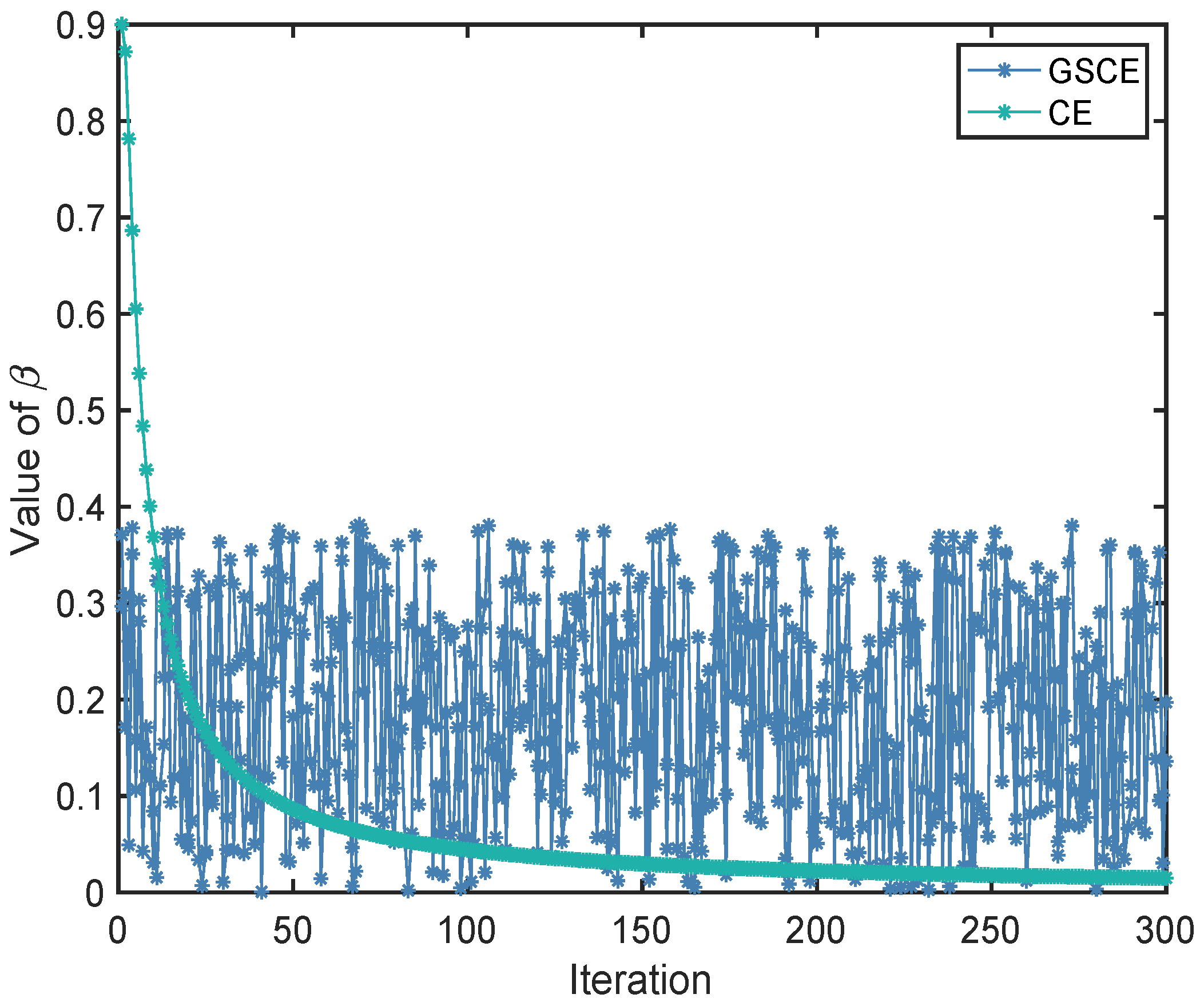
The parameter β also affects the convergence speed of CE method. According to the simulation results discussed in Section 4, a small β may slow down the convergence process. In GSCE, β is limited to 0 , 0.382 which is much smaller than that in (46), hence to slow down the convergence process. Value of β for GSCE and CE in each iteration are plotted in Figure 2.
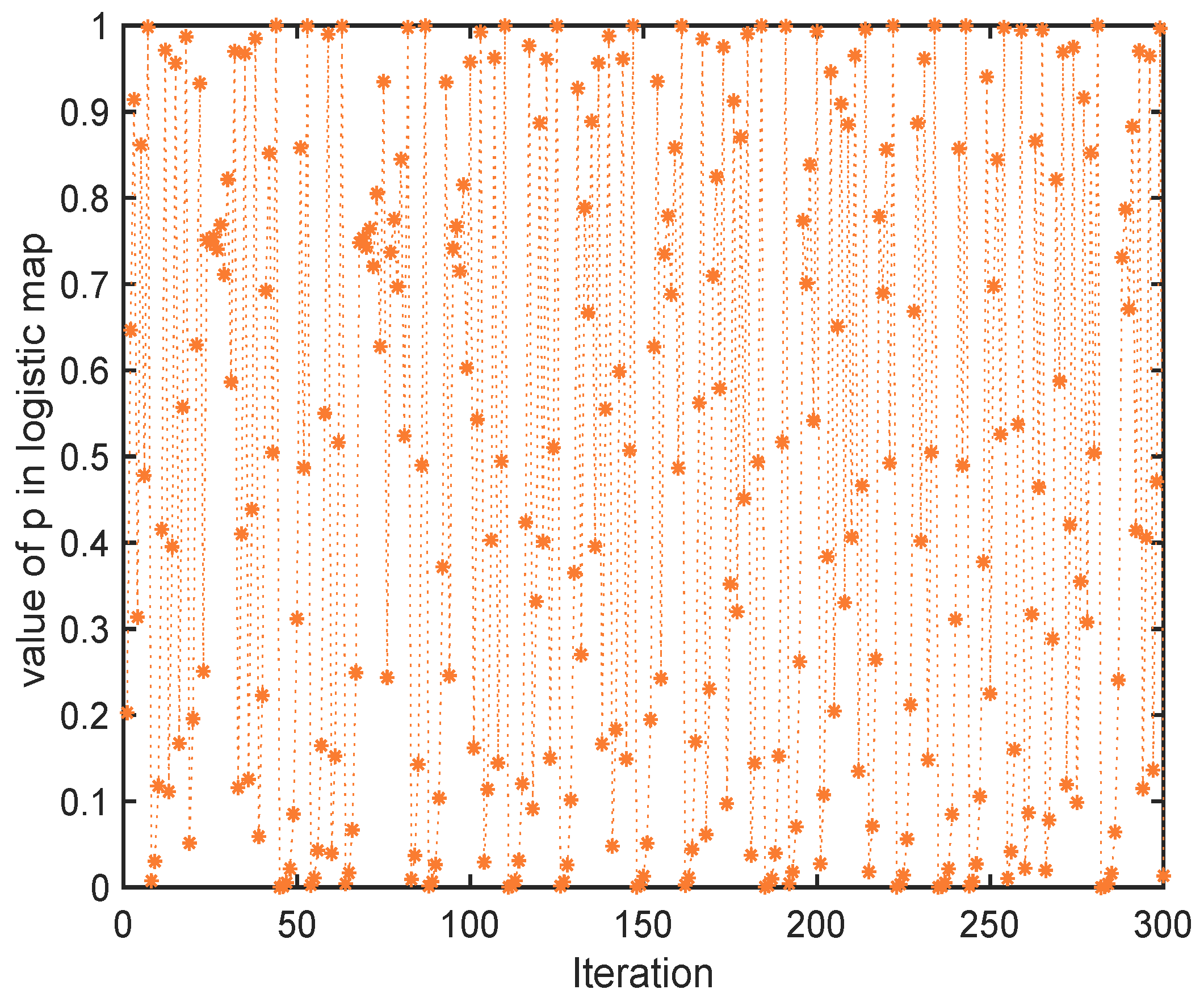
To improve the exploration ability of CE method, the chaotic operator [42] in CGSCE is used to determine β . Logistic map is selected as chaotic operator defined in (49), the parameter α in smoothed updating process is set to 1, β is calculated as follows:
p t = 4 p t 1 1 p t 1 , t = 2 ,
β t = 0.382 μ , i f γ < p t β β ( 1 1 t ) q , e l s e
where p t is the probability used to determine the form of β in generation t, p 1 = 0.2027 . μ and γ are random numbers generated under the uniform distribution U 0 , 1 , q is an integer typically between 5 and 10.
The plot of chaotic sequences of Logistic map is given in Figure 3. It is obvious that chaotic sequences of Logistic map locate between 0 and 1 irregularly. The advantages of introduction of chaotic operator into proposed can be concluded as follows:
  • In the initial stage of the algorithm, CGSCE has chance to acquire a big value of β due to the probabilistic selection of (41) to renew β while β in GSCE is limited to 0 , 0.382 , so CGSCE has chance to converge faster than GSCE in initial stage.
  • In the final stage of the algorithm, CGSCE has chance to acquire a bigger value of β than that in CE method given by (41).
  • A large perturbation of β generated by chaotic operator can improve the exploration ability of CGSCE.

3.2.3. Archive

According to the simulation results, the best solutions of each iteration in CGSCE are not always decrease monotonically. In other words, the best solution in the final iteration is not always the best solution among all iterations. In CGSCE, the best solution in first generation is preserved in an archive. In subsequent generations, if there exists a solution better than the solution in archive, it will be added to the archive and previous solution in archive will be removed, otherwise the solution in archive will remain the same. This can be done by using SF to select best individual between current best individual and previous solution in archive. In the final iteration, the solution in archive is regarded as the best solution.

3.3. Constraints Handling

Constraints handling method of CGSCE is introduced in this subsection including constraints handling for control variables, calculation of total constraints violation and superiority of feasible solutions. The pseudo-code for calculating the total constraints violation and SF are also given in this subsection.

3.3.1. Constraints Handling for Control variables

In CGSCE, population is created under the normal distribution, some individuals may be out of feasible range. To avoid violation of control variables, infeasible individuals is repaired as soon as population is generated according following formula:
X i j = X m i n j , i f X i j < X m i n j X m a x j , i f X i j > X m a x j
where X i j is jth component of individual X i , X m i n j is the lower bound of jth component of population, X m a x j is the upper bound of jth component of population.

3.3.2. Calculation of Total Constraints Violation

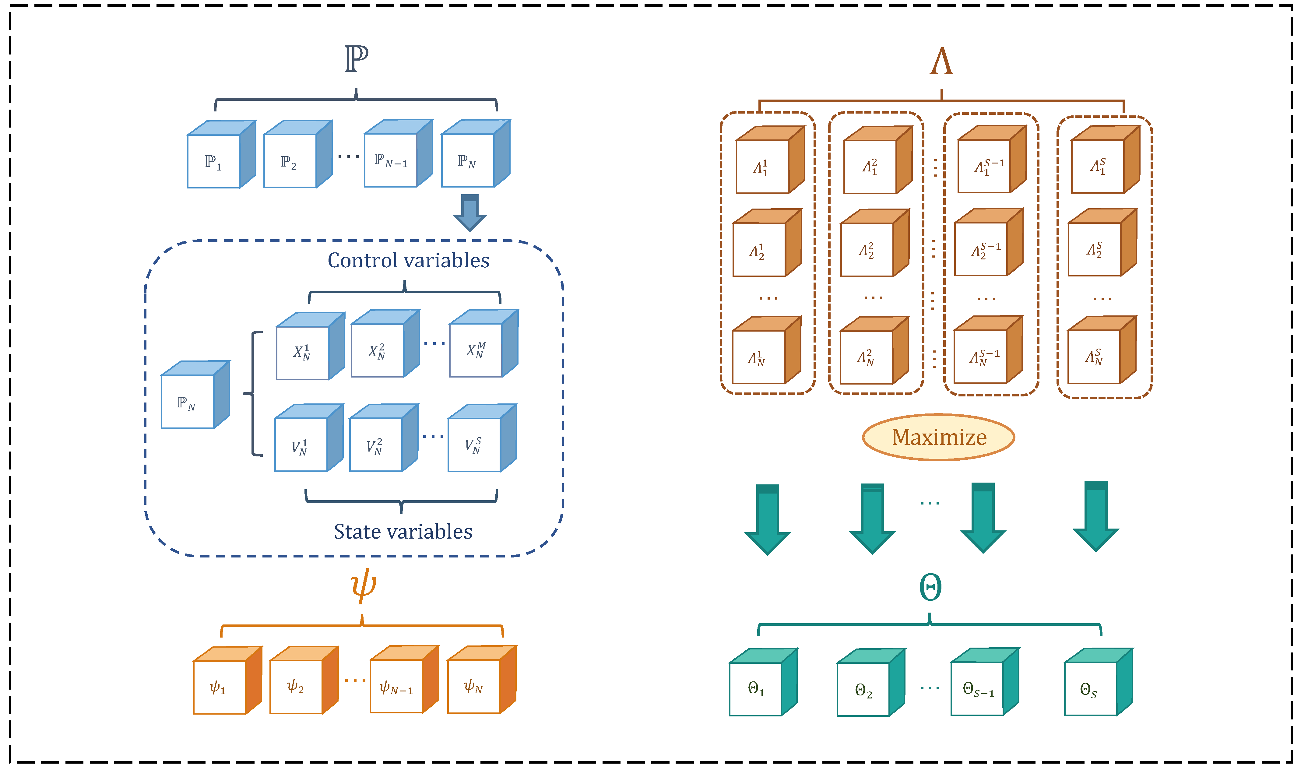
Calculation of total constraint violation is implemented when objective function has been evaluated and state variables have been acquired. Figure 4 illustrate the structure of variables existing in calculation of total constraints violation, where P is population, ψ records normalized constraints violation of all individuals, Λ records all constraints violation of state variables in the population, M is the number of control variables, S is the number of state variables. Θ records all maximum constraints violation of each state variables in Λ . It should be noticed that infeasible control variables have been repaired before performing power flow calculation, so the total constraint violation is only attributed to states variables.
Constraint violation of each state variable in OPF problems is calculate by:
Λ i j = V m i n j V i j , i f V i j < V m i n j V i j V m a x j , i f V j j > V m a x j
where Λ i j is the constraints violation of jth state variable of individual i, V m i n j and V m a x j are the lower bound and upper bound of jth state variable respectively.
The process of calculating total constraints violation is shown as follows:
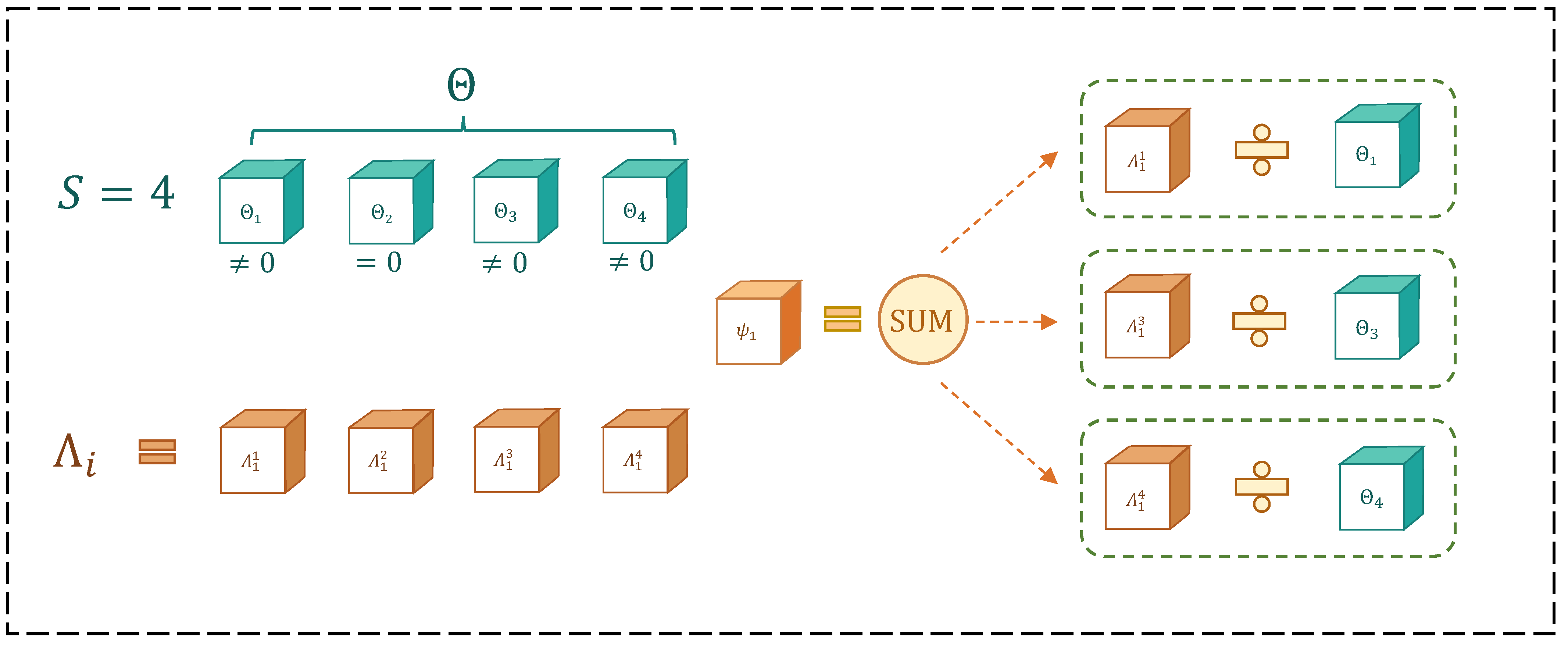
In the beginning, all elements in ψ are set to 0. Then both state variable constraints violation of each individual and all maximum constraint violation of corresponding each state variables are recorded in Λ and Θ respectively. The number of infeasible individuals may become zero after several iterations. In order to avoid unnecessary operations, only if an infeasible individual exists in the current population will the calculation of the constraint violation be implemented. This is same that we only calculate the constraints violation of infeasible individuals. In order to make all state variables have fair contribution to total constraints violation, it is necessary to normalize them. This can be done by using constraints violation of ith state variable of an individual divided by maximum constraints violation of corresponding state variables of the population. The obtained result is used as normalized constraints violation of ith state variable of an individual. Due to the denominator of normalized constraints violation is the component of Θ , the obtained normalized constraints violation will become infinity when a component of Θ is 0. Furthermore, if a component of Θ is 0, it means all individuals does not violate corresponding state variable. So, if a component of Θ is 0, calculation violation of corresponding state variable must be neglected.
Figure 5 gives an example of the calculation of normalized constraints violation when the number of state variables is S = 4 . The second component of Θ is zero implies that all individuals do not violate the constraints of second state variable. So, the calculation of normalized constraints violation of second state variable is omitted in the calculation of ψ 1 .
The pseudocode for calculating the total constraints violation is given in Algorithm 2. where δ is the set of indices of state variable. μ used to record the index of infeasible individual in P .
Algorithm 2 Algorithm for Calculating Total Constraints Violation (totalViolation)
  1:
set all elements in Ψ to 0
  2:
record each constraint violation of state variables of p to Λ
  3:
record all maximum constraints violation corresponding to each state variable in p to Θ
  4:
if Θ has a non-zero element then
  5:
    for each infeasible individual i μ  do
  6:
          for each j δ which satisfy Θ j 0  do
  7:
                Ψ i Ψ i + Λ i j / Θ j
  8:
          end for
  9:
    end for
10:
end if

3.3.3. Superiority of Feasible Solutions

Superiority of feasible solutions is a constraint handling method proposed by Deb [34]. In our approach, SF is used to handle infeasible state variables. In SF, two solutions X 1 and X 2 use the following rule to compare: X 1 is considered better than X 2 if the violation of X 1 is less than X 2 or the violation of X 1 and X 2 is equal and the fitness of X 1 is better than X 2 .
The SF is performed when power flow calculation has been conducted and the fitness of population has been achieved. As shown in Algorithm 1, CE method utilizes elite individuals to renew the parameters of normal distribution. In other words, the search direction of CE method is based on the elite individuals. In the initial stage, the low constraint violation individuals are used to direct the search direction under the rule of SF and the search region moves toward low constraint violation region. As the iteration of algorithm, more and more feasible individuals exist in the population and finally all top N e l i t e individuals in population are feasible. In this situation, the top N e l i t e individuals with best fitness are used to direct the search direction and search region moves toward the fittest region. The pseudocode of SF is given in Algorithm 3 where f . is objective function, p ρ is the sorted population.
Algorithm 3 Algorithm for Superiority of Feasible Solutions (SF)
  1:
sort Ψ in ascending order, record the sorted value and index to C and γ respectively
  2:
record the element of C without repetition to Φ
  3:
ρ
  4:
for each element in Φ  do
  5:
    add element of γ which violation is equal to current element of Φ to υ
  6:
    if  υ  then
  7:
        sort f p υ in ascending order and add the sorted index to ρ .
  8:
    end if
  9:
end for
10:
p p ρ

3.4. CGSCE for Solving OPF Problem

MATPOWER is an open-source software package for solving steady-state power system simulation [43]. In this paper, the power flow calculation is implemented by MATPOWER 7.1. The pseudocode of CGSCE for Solving OPF Problem is given in Algorithm 4, where G b e s t records the global best individual, D records the the information of control variables, state variables and other information used to calculate the power flow, D c o n t r o l is the control variables in D , X is the control variables of population P , X m i n i and X m a x i are the low bound and upper bound of ith control variable, M is a MATPOWER options variable, R records the result of power flow calculation, R c o n t r o l and R s t a t e are the control variables and state variables in R respectively. F records the fitness of a population. The algorithm including following functions:
  • initialize. The initialize function is used to initialize the parameters of the algorithm including: N: population size, N e l i t e : number of elite individuals, M a x F e s : maximum function evaluations, F e s = 0 : current function evaluations, α = 0.8 , β = 0.9 , q = 5 , t = 0 : iteration number and p = 0.2027 is the initial value of chaotic operator.
  • mpoption. The mpoption is a function of matpower used to set and retrieve a MATPOWER options variable. More details information about mpoption, please refer to the source code of MATPOWER.
  • loadcase. The loadcase is a function of MATPOWER used to load the data of a specific test system. This function return a structure variable contains the information control variables, state vaiables and other information used to calculate power flow.
  • runpf. The runpf is a function of MATPOWER used to run a power flow, it returns a variable D contains the control variables X and state variables V.
The algorithm is initialized from step 1 to step 9 and iterates between step 10 and step 30. The main process of iteration can be divided by three parts: Part 1: generate population. Part 2: evaluate population. Part 3: renew the parameters of the algorithm. In step 12, each control variable of each individual is renewed by the normal distribution. In step 15, the control variables of population is assigned to D c o n t r o l and then D is used for the calculation of power flow as shown in step 16. The fitness of population F can be calculate by R c o n t r o l and R s t a t e according to the objective function as shown in step 18. The total constraint violation of population can be achieved by formula (46) and Algorithm 2. After the fitness of population F and total constraint violation of population Ψ are achieved, population is sorted by SF using Algorithm 3. Then the elite individuals are used for renewing the parameters of normal distribution as shown in part 3, hence to direct the search direction. The algorithm will terminate when the function evaluation F e s is equal or large to the M a x F e s .
Algorithm 4 CGSCE for Solving OPF Problem
  1:
initialize
  2:
G b e s t
  3:
D loadcase (test system datas)
  4:
M mpoption ( )
  5:
//initialize the parameters of the normal distribution
  6:
for i = 1 to M do
  7:
     μ l i = μ c i = X m i n i + r a n d × ( X m a x i X m i n i )
  8:
     σ l i = σ c i = 10 × ( X m a x i X m i n i )
  9:
end for
10:
while F e s < M a x F e s do
11:
    //Part 1: generate population
12:
    renew each control variable i of each individual j by: X j i = N μ l i , σ l i
13:
    repair X using (45)
14:
    //Part 2: evaluate population
15:
     D c o n t r o l X
16:
     R runpf ( M , D )
17:
     V R s t a t e
18:
    calculate F by R c o n t r o l and R s t a t e according to the objective function
19:
    calculate Λ by V using (46)
20:
     Ψ totalViolation ( Λ )
21:
     P SF ( P G b e s t , Ψ , F )
22:
     G b e s t P 1
23:
    //Part 3: renew the parameters of algorithm
24:
    for  i = 1 to M do
25:
         μ c i 1 N e l i t e j = 1 N e l i t e X j i , σ c i 1 N e l i t e j = 1 N e l i t e X j i μ c i 2
26:
    end for
27:
     p 4 × ( 1 p ) ,     t t + 1 ,    F e s F e s + N
28:
    renew p and β according to (43) and (44) respectively
29:
     σ l β × σ c + ( 1 β ) × σ l , μ l μ c
30:
end while

4. Study Cases and Simulation Results

Study cases and simulation results of applying the proposed algorithm to the IEEE-30 bus system and IEEE-57 bus system will be presented and discussed in this section. To show the effectiveness of CGSCE in solving OPF problem, CE, GSCE and several algorithms reported in the literature are used for comparison. Furthermore, in order to investigate the convergence performance of CGSCE, graphical comparison of three CE methods are also given. The proposed method is coded in Matlab language and run on a computer with Intel Core i7 CPU @2.6 GHz and 16 GB RAM.

4.1. Study Cases for IEEE-30 Bus System

Several study cases for IEEE-30 bus system will be introduced in this subsection. The one line diagram of IEEE-30 bus system [44] is plotted in Figure 6. IEEE-30 bus system has 6 generators, 24 load buses, 41 branches, 4 transformers and 9 shunt VAR compensators. One of the 6 generators is swing generator used to balance the power in system. According (4) and (5), it is evident that the IEEE-30 bus system has 24 control variables.

4.1.1. Case1: Minimization of Fuel Cost

Fuel cost can be formulated as a quadratic function as follows:
F c x , v = i = 1 N g a i + b i P G i + c i P G i 2
where F c x , v is total fuel cost, a i , b i , c i are fuel cost coefficients of ith generator. Coefficients of all generators in the IEEE-30 bus system are listed in Table A1.

4.1.2. Case 2: Minimization of Fuel Cost Considering Multiple Fuels

In practical power system operation, thermal generating units may be supplied by multiple fuel source likes coal, natural gas and oil [1]. In this situation, the characteristic of fuel cost function becomes piece-wise quadratic as shown in Figure 7, which makes problem becomes a non-convex optimization one. The formulation of fuel cost is modified as follows:
F c x , v = i = 1 N g a i , k + b i , k P G i + c i , k P G i 2 , i f P G i , k m i n P G i P G i , k m a x
where F c x , v is total fuel cost, k is the type of fuel, a i , k , b i , k c i , k are the coefficients of fuel cost of ith generator with fuel k when active power output lies in [ P G i , k m i n , P G i , k m a x ] .
In this paper, multiple fuels option is considered for generator 1 and generator 2, the remaining generator are same as Case 1. Coefficient and corresponding power outputs of generators are listed in Table A2.

4.1.3. Case 3: Minimization of L-Index

L-index proposed by Kessel and Glavitsh in 1986 is used as an indicator for voltage stability in power system [35]. The value of L-index varies in range between 0 and 1, where 0 indicate no-load of system and 1 indicate voltage collapse. L m a x as an indicator for the stability of a power system can be expressed as [1]:
L m a x = m a x L k , k = 1 , 2 , , N l

4.1.4. Case 4: Minimization of Emission

A large amount of emissions like carbon dioxide are produced when thermal power plants are in operation. The relationship between emissions and active power output can be described as:
F e x , v = i = 1 N g α i + β i P G i + γ i P G i 2 × 0.001 + ω i e μ i P G i
where α i , β i , γ i , ω i , μ i are emission coefficients listed in Table A2.

4.1.5. Case5: Minimization of Active Power Loss

Active power loss in transmission line can be formulated as [36]:
F p x , v = i = 1 N l j i N l G i j V i 2 + V j 2 2 V i V j c o s ( δ i δ j )
where V i is voltage magnitude of ith load bus, δ i is voltage angle ith bus, G i j is the transfer conductance between bus i and bus j.

4.2. IEEE-30 Bus System Simulation Results

In this subsection, the objective of different study cases for IEEE-30 bus system are described in Table 1. CGSCE, GSCE, and CE and are all run 30 times in each study case and 30000 function evaluations (Fes) used as their termination criterion in each run for IEEE-30 bus system. Parameters setting of these three CE methods are listed in Table 2.

Simulation Results of CGSCE, GSCE and CE for IEEE-30 Bus System

The results of three CE methods in different study cases for IEEE-30 bus system are presented in Table 3. Each case contains Min, Avg and Max three columns represent minimum value (best value), average value and maximum value (worst value) in 30 runs of each algorithm correspondingly. CGSCE outperformed GSCE in all study cases except for Case 4 in IEEE-30 bus system. In Case 2, CGSCE has much lower average value and maximum value than GSCE. Three CE methods have similar results in Case 4 which aims to minimize emission only. This phenomenon may be attributed to the emission coefficient such as ω i and 0.01 in formula (50) is quite small which in turn to makes final emission value become small. Although CE offer a lower minimum value than CGSCE in Case 2, the difference between CE and CGSCE in this case is only 0.07%. Moreover, CGSCE perform well in average value and maximum value than CE in Case 2. It can be concluded that CGSCE has better performance than other two CE methods in most of cases for the IEEE-30 bus system.
The standard deviation of results and average simulation time of three CE methods in 30 runs for IEEE-30 bus system are provided in Table 4. The average simulation time among three CE methods is quite similar in all 5 cases. The lowest standard deviation of Case 1 and Case 2 among 30 runs can be achieved by CGSCE while CE perform best in Case 4 and Case 5 for providing the lowest standard deviation.
The best solutions in 30 runs of CGSCE, GSCE and CE in study Case1 to Case 5 of IEEE-30 bus system are detailed in Table 5 and Table 6 respectively. In these two tables, columns labeled by Min and Max records the lower bound and upper bound of control variables and state variables correspondingly.
According to Table 5 and Table 6, all three CE methods do not violate both control variables and state variables using SF. As revealed in the simulation results, discrepancy of control variables among these algorithms is quite small in Case 1, Case 2, Case 4 and Case 5 which in turn makes them have similar state variables and objective values. In Case 3, the discrepancy among three CE methods is large than other 4 cases for the IEEE-30 bus system.
The power output of a generator, the only parameter included in the calculation of fuel cost and emission should be discussed in detail. It seems that a higher fuel cost implies a higher emission. However, a counterexample appears in Case 3 between CE and GSCE where the fuel cost of GSCE is less than CE, but the emission of GSCE is higher than CE. This phenomenon can be attributed to the discrepancy among generator cost coefficient and emission coefficient. Moreover, the active power output given by these two algorithms is quite different. In Case 1 and Case 2, three CE methods gave similar result for active power output of generator which in turn to reduce difference of fuel cost and emission.
Box plots of three CE methods for Case1 and Case2 are given in Figure 8. The best results in each 30 runs of each CE method are used for box plots. It is clear that CGSCE outperformed than other two CE methods in minimum value, average value and maximum value in Case1. Furthermore, CGSCE is much robust than other two CE methods in Case1. In Case2, although three CE methods provided similar results in minimum value and average value, CGSCE is obvious much more robust than the other two CE methods for providing much smaller maximum value in 30 runs.
Table 7 gives the comparison results of CGSCE and other algorithms for Case 1. CGSCE performed best among these algorithms for providing least fuel cost.
Comparision results of Case 2 is shown in Table 8. It is evident that CGSCE outperform than other algorithms in both aspects of fuel cost and power loss. Meanwhile, three CE methods and MSA provided similar results in this case.
Table 9 provides the comparison results of Case 3, which aims to minimize the L-index of a power system. CE gave the best performance among all algorithms in this case. However, the fuel cost provided by CE is much worse than two other CE methods. Although GSCE provided best solution of fuel cost in Case 3, the emission and power flow provided by GSCE is much worse than other two CE methods.
Table 10 is the comparison results of Case 4 which aims to minimize the emission. Due to the small coefficients for the emission, results provided by all algorithms is quite similar. Among these algorithms, three CE methods, MSA and SF-DE performed best with 0.20482 (t/h) of emission. Meanwhile, three CE methods gave excellent results in fuel cost which means a less generating cost.
Simulation results of Case 5 are detailed in Table 11. In this case, the main goal of OPF is to minimize the active power loss. As mentioned before, reducing active power loss of transmission line will save the cost of generating. It is obvious that CGSCE outperformed other algorithms in power loss. Other two CE methods named GSCE and CE gave second and the third best result in power loss in this case respectively. Moreover, the voltage deviation provided by CGSCE also outperformed other algorithms.

4.3. Study Cases for IEEE-57 Bus System

The one line diagram of IEEE-57 bus system [52] is plotted in Figure 9. The IEEE-57 bus system has 7 generators, 50 load buses, 80 branches, 17 transformers and 3 shunt VAR compensators. Among these 7 generators, the first generator is swing generator. Hence, an IEEE-57 system has 33 control variables according to (4) and (5). In this section, several study cases based on IEEE-57 bus system are introduced.

4.3.1. Case 6: Minimization of Fuel Cost

In this study case, the quadratic fuel cost is used as the objective function of OPF similar to Case 1. The formula of basic quadratic fuel cost in IEEE-57 bus system can be calculated by (47). It should be noted that IEEE-57 bus system contains 7 generators different from the IEEE-30 bus systems. As a result, the value of N g is 7 in IEEE-57 system.

4.3.2. Case 7: Minimization of Voltage Deviation

Voltage deviation is used as an indicator for the service quality of a power system. In order to improve voltage profile, deviation of load buses voltage from the unity should be minimized [36]. The total voltage deviation can be calculated as follows:
F v d x , v = i = 1 N l V L i 1

4.4. IEEE-57 Bus System Simulation Results

Simulation results of IEEE-57 bus system are provided in this subsection. Objectives of Case 6 and Case 7 for IEEE-57 bus system are minimization of fuel cost and voltage deviation respectively. CGSCE, GSCE, and CE and are all run 30 times in each study case and 42,000 function evaluations (Fes) used as their termination criterion in each run for IEEE-57 bus system.

4.4.1. Simulation Results of CGSCE, GSCE and CE for IEEE-57 Bus System

Comparison results for the three CE methods for IEEE-57 bus system are listed in Table 12. The main goal of Case 6 is to minimize the basic quadratic fuel cost in IEEE-57 bus system. In this case, CGSCE outperformed the other two CE methods in providing minimum value. In Case7, the best result was achieved by CGSCE with 0.5880 (p.u.).
The standard deviation of results and average simulation time of three CE methods in 30 runs for IEEE-57 bus system are provided in Table 13. Similar to the results in IEEE-30 bus system, the average simulation time among three CE methods is quite similar in 2 cases of IEEE-57 bus system. It should be noticed that the maximum function evaluation is 42,000 in IEEE-57 bus system while 30,000 in IEEE-30 bus system. It means the algorithm iterates more times in IEEE-57 bus system than that in IEEE-30 bus system. The lowest standard deviation of Case 6 and Case 7 among 30 runs can be achieved by CE.
Figure 10 shows the voltage profile of load buses provided by CGSCE in Case 7. According to Figure 10, the voltage of all load buses fluctuates around 1 p.u. with small deviations which means the voltage is distributed equally in load buses.
Best solutions provided by the three CE methods are given in Table 14. Similar to Case 1 of IEEE-30 bus system, fuel cost in Case 6 of IEEE-57 bus system among three CE methods are quite similar to each other. As shown in Table 14, the least fuel cost can be achieved by CGSCE. Meanwhile, CGSCE also provided a less emission solution. In Case 7, CGSCE outperformed the other two CE methods in both voltage deviation and L-index. Further, the best solution of three CE methods do not violate any constraint of OPF while using SF as constraint handling technique.

4.4.2. Comparision of The Simulation Results for IEEE-57 Bus System

In this section, CGSCE have been compared with other algorithms for IEEE-57 bus system. Comparison results of the best solutions for case 6 is listed in Table 15. In this case, CGSCE outperformed the other algorithms which gives the best fuel cost of 41,667.2777 ($/h). CE gave second best fuel cost results of 41,669.0222 ($/h). In Table 16, simulation results of Case 7 are given. It is evident that CGSCE outperformed the other algorithms for providing much less voltage deviation results.

4.5. Comparison of Convergence Performance

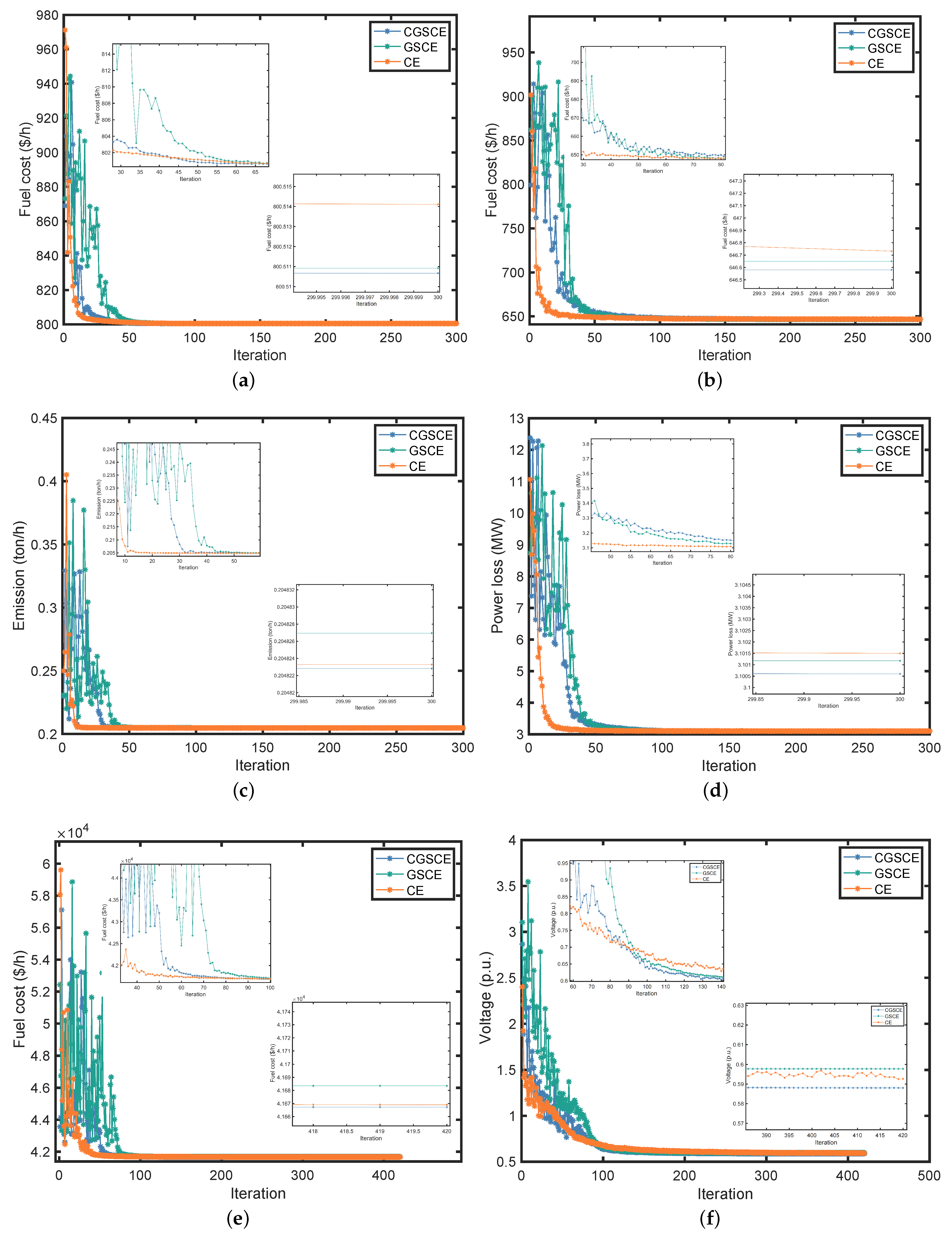
The convergence performance of the three CE methods in Case 1, Case 2, Case 4 and Case 5 for IEEE-30 bus system are plotted in Figure 11a–d respectively. The total function evaluations of three CE methods in a run is set to 30,000 and the population size of each CE method is set to 100. Accordingly, every iteration of CE methods needs 100 function evaluations and all algorithms will terminate after 300 iterations. It is evident that GSCE exhibited greater fluctuations than CGSCE and CE in the initial stage of these 4 cases. Furthermore, CGSCE converged to near optimal solution faster than GSCE in these 4 cases due to the introduction of the chaotic operator and GSCE is obvious worse than other two CE methods in this aspect. The fast convergence of three CE methods can be observed in Case1 and Case 4 where all CE methods can almost converge to the best obtained result within 50 iterations.
Figure 11e,f illustrate the convergence property of three CE methods in Case 6 and Case 7 for IEEE-57 bus system correspondingly. In IEEE-57 bus system, the maximum function evaluation of each CE method in a run is 42,000, the population of each CE method is set to 100. So, each CE method will iterate 420 times in a run. Similar to the circumstance appears in IEEE-30 bus system, GSCE showed greater fluctuation than CGSCE and CE in Case 6 and Case 7. No obvious difference of the best results of Case 6 obtained by CGSCE and CE is observed but solution obtained by GSCE is obviously worse than CGSCE and CE. It is clear that all the three CE methods need more iterations to converge to nearly best result in Case 7 than that in Case 6.
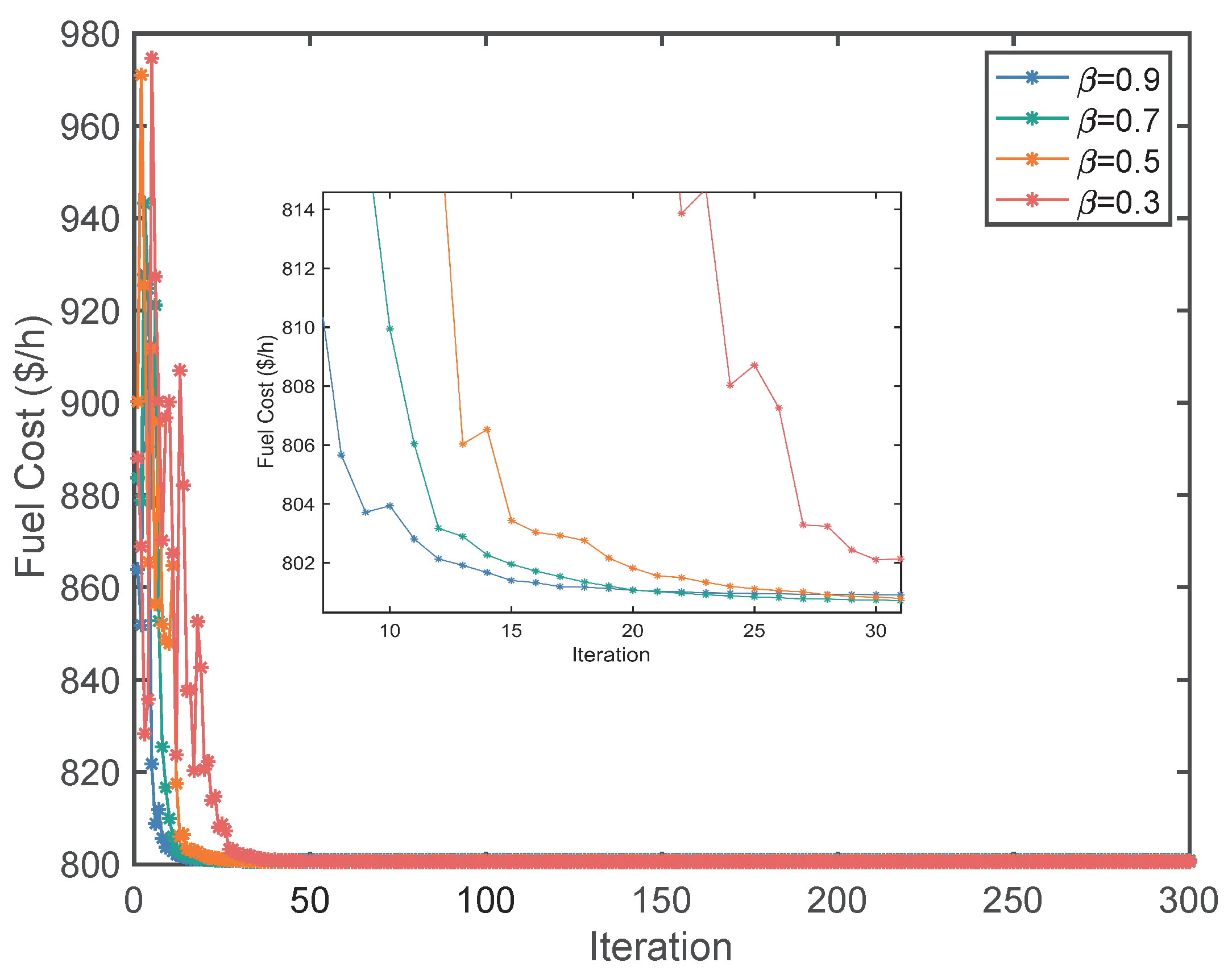
The convergence property of CE method with different β is plotted in Figure 12. The parameter α are all set to 1 and beta are set to 0.9, 0.7, 0.5 and 0.3 respectively. All cases are run 30 times and the best solution among these 30 runs are used for plotting. As mentioned before, β will influence the convergence speed of algorithm. It’s clear that the lager β is, the faster CE method will converge to near optimal solution.

5. Conclusions

This paper describes the application of an improved cross-entropy method named CGSCE to solve optimal power flow problems. The proposed method has been tested on both IEEE-30 bus system and IEEE-57 bus system with 7 different study cases. The study considers the minimization of fuel cost, voltage deviation, emission, active power losses and L-index. In order to show the efficiency of CGSCE in solving OPF problems, CGSCE has been compared with other algorithms report in literature. Simulation results shows that CGSCE has competitiveness in solving OPF problems. Furthermore, proposed method can provide no constraint violation individuals using SF as constraint handling technique which means power system can operate in security. CGSCE has also been compared with two other CE methods to show the efficiency of proposed innovation. Simulation results shows that the introduction of chaotic operator can improve both the convergence speed and exploration capability of proposed method.
Future research work including using CE method to solve muti-objective OPF problems, many-objecticve OPF problems, probabilistic optimal power flow problems and OPF problems considering renewable source.

Author Contributions

Q.N. designed the research, H.S. and Q.N. proposed the innovation, H.S., Q.N. and Z.Y. performed and analyzed the experience, H.S., Q.N. and Z.Y. wrote the paper, Q.N., H.S. and Z.Y. revised the paper. All authors have read and agreed to the published version of the manuscript.

Funding

This research was funded by China NSFC (61773252, 62003332) and Outstanding Young Researcher Innovation Fund of Shenzhen Institute of Advanced Technology, Chinese Academy of Sciences (201822).

Institutional Review Board Statement

Not applicable.

Informed Consent Statement

Not applicable.

Data Availability Statement

No new data were created or analyzed in this study. Data sharing is not applicable to this article.

Acknowledgments

There is no any support which is not covered by the author contribution or funding sections.

Conflicts of Interest

The authors declare that there is no conflict of interests regarding the publication of this paper.

Abbreviations

The following abbreviations are used in this manuscript:
OPFOptimal power flow
CECross-entropy method
CGSCEImproved cross-entropy method assisted with a chaotic operator
GSCEGolden stochastic linear cross-entropy method
SOPFSecurity-constrained optimal power flow
DOPFDynamic optimal power flow
CHConstraints handling
SFSuperiority of feasible solution
GAGenetic Algorithm
DEDifferential Evolution
PSOParticle Swarm Optimization
HSAHarmony Search Algorithm
TLBOTeaching-learning-Based Optimization
ABCArtificial Bee Colony Optimization
MSLFAShuffle Frog Leaping Algorithm
MICAModified Imperialist Competitive Algorithm
ARCBBOAdaptive Real Coded Biogeography-based Optimization
ASPAssociated stochastic problem
MLEMaximum likelihood estimation
CDFCumulative distribution function

Appendix A

Table A1. Cost coefficients of all generators for IEEE-30 bus system.
GeneratorBusabcde α β γ ω μ
G 1 1020.00375180.0374.091−5.5546.490.00022.857
G 2 201.750.0175160.0382.543−6.0475.6380.00053.333
G 3 5010.0625140.044.258−5.0944.5860.0000018
G 4 803.250.00834120.0455.326−3.553.380.0022
G 5 11030.025130.0424.258−5.0944.5860.0000018
G 6 13030.02513.50.0416.131−5.5555.1510.000016.667
Table A2. Cost coefficients of generators 1 and 2 for IEEE-30 bus system considering multiple fuels.
GeneratorBus P G i , 1 min P G i , 1 min abc P G i , 2 min P G i , 2 max abc
G 1 150140550.70.00514020082.51.050.0075
G 2 22055400.30.015580800.60.02

References

  1. Abou El Ela, A.A.; Abido, M.A.; Spea, S.R. Optimal power flow using differential evolution algorithm. Electr. Power Syst. Res. 2010, 80, 878–885. [Google Scholar] [CrossRef]
  2. Zhang, J.R.; Tang, Q.H.; Li, P.; Deng, D.X.; Chen, Y.L. A modified MOEA/D approach to the solution of multi-objective optimal power flow problem. Appl. Soft Comput. 2016, 47, 494–514. [Google Scholar] [CrossRef]
  3. Biswas, P.P.; Suganthan, P.N.; Mallipeddi, R.; Amaratunga, G.A.J. Multi-objective optimal power flow solutions using a constraint handling technique of evolutionary algorithms. Appl. Soft Comput. 2020, 24, 2999–3023. [Google Scholar] [CrossRef]
  4. Frank, S.; Steponavice, I.; Rebennack, S. Optimal power flow: A bibliographic survey I. Energy Syst. 2012, 3, 221–258. [Google Scholar] [CrossRef]
  5. Vaisakh, K.; Srinivas, L.R. Evolving ant direction differential evolution for OPF with non-smooth cost functions. Eng. Appl. Artif. Intell. 2011, 24, 426–436. [Google Scholar] [CrossRef]
  6. Holland, J.H. Adaptation in Natural and Artificial Systems; University of Michigan Press: Ann Arbor, MI, USA, 1975. [Google Scholar]
  7. Storn, R.; Price, K. Differential evolution—A simple and efficient heuristic for global optimization over continuous spaces. J. Glob. Optim. 1997, 11, 341–359. [Google Scholar] [CrossRef]
  8. Kennedy, J.; Eberhart, R. Particle Swarm Optimization. In Proceedings of the ICNN’95—International Conference on Neural Networks, Perth, Australia, 1 December 1995; pp. 1942–1948. [Google Scholar]
  9. Geem, Z.W.; Kim, J.H.; Loganathan, G.V. A New Heuristic Optimization Algorithm: Harmony Search. Simulation 2001, 2, 60–68. [Google Scholar] [CrossRef]
  10. Rao, R.V.; Savsani, V.J.; Vakharia, D.P. Teaching-learning-based optimization: A novel method for constrained mechanical design optimization problems. Comput. Aided Des. 2011, 43, 303–315. [Google Scholar] [CrossRef]
  11. Karaboga, D. An Idea Based on Honey Bee Swarm for Numerical Optimization; Technical Report-TR06; Erciyes University, Engineering Faculty, Computer Engineering Department: Kayseri, Turkey, 2005. [Google Scholar]
  12. Niknam, T.; Narimani, M.R.; Jabbari, M.; Malekpour, A.R. A modified shuffle frog leaping algorithm for multi-objective optimal power flow. Energy 2011, 36, 6420–6432. [Google Scholar] [CrossRef]
  13. Narimani, M.R.; Azizipanah-Abarghooee, R.; Zoghdar-Moghadam-Shahrekohne, B.; Gholami, K. A novel approach to multi-objective optimal power flow by a new hybrid optimization algorithm considering generator constraints and multi-fuel type. Energy 2013, 49, 119–136. [Google Scholar] [CrossRef]
  14. Ghasemi, M.; Ghavidel, S.; Rahmani, S.; Roosta, A.; Falah, H. A novel hybrid algorithm of imperialist competitive algorithm and teaching learning algorithm for optimal power flow problem with non-smooth cost functions. Eng. Appl. Artif. Intell. 2014, 29, 54–69. [Google Scholar] [CrossRef]
  15. Adaryani, M.R.; Karami, A. Artificial bee colony algorithm for solving multi-objective optimal power flow problem. Int. J. Electr. Power Energy Syst. 2013, 53, 219–230. [Google Scholar] [CrossRef]
  16. Roy, R.; Jadhav, H.T. Optimal power flow solution of power system incorporating stochastic wind power using Gbest guided artificial bee colony algorithm. Int. J. Electr. Power Energy Syst. 2015, 64, 562–578. [Google Scholar] [CrossRef]
  17. Shabanpour-Haghighi, A.; Seifi, A.R.; Niknam, T. A modified teaching-learning based optimization for multi-objective optimal power flow problem. Energy Convers. Manag. 2014, 77, 597–607. [Google Scholar] [CrossRef]
  18. Ghasemi, M.; Ghavidel, S.; Gitizadeh, M.; Akbari, E. An improved teaching-learning-based optimization algorithm using Levy mutation strategy for non-smooth optimal power flow. Int. J. Electr. Power Energy Syst. 2015, 65, 375–384. [Google Scholar] [CrossRef]
  19. Kumar, A.R.; Premalatha, L. Optimal power flow for a deregulated power system using adaptive real coded biogeography-based optimization. Int. J. Electr. Power Energy Syst. 2015, 73, 393–399. [Google Scholar] [CrossRef]
  20. Biswas, P.P.; Suganthan, P.N.; Mallipeddi, R.; Amaratunga, G.A.J. Optimal power flow solutions using differential evolution algorithm integrated with effective constraint handling techniques. Eng. Appl. Artif. Intell. 2018, 68, 81–100. [Google Scholar] [CrossRef]
  21. Warid, W.; Hizam, H.; Mariun, N.; Abdul-Wahab, N.I. Optimal Power Flow Using the Jaya Algorithm. Energies 2016, 9, 678. [Google Scholar] [CrossRef] [Green Version]
  22. Chen, G.G.; Lu, Z.M.; Zhang, Z.Z. Improved Krill Herd Algorithm with Novel Constraint Handling Method for Solving Optimal Power Flow Problems. Energies 2018, 11, 76. [Google Scholar] [CrossRef] [Green Version]
  23. Rubinstein, R. The Cross-Entropy Method for Combinatorial and Continuous Optimization. Methodol. Comput. Appl. 1999, 1, 127–190. [Google Scholar] [CrossRef]
  24. Wang, G.B.; Zha, Y.X.; Wu, T.; Qiu, J.; Peng, J.C.; Xu, G. Cross entropy optimization based on decomposition for multi-objective economic emission dispatch considering renewable energy generation uncertainties. Energy 2020, 193, 982–997. [Google Scholar] [CrossRef]
  25. Selvakumar, A.I. Enhanced cross-entropy method for dynamic economic dispatch with valve-point effects. Int. J. Electr. Power Energy Syst. 2011, 33, 783–790. [Google Scholar] [CrossRef]
  26. Carvalho, L.D.; da Silva, A.M.L.; Miranda, V. Security-Constrained Optimal Power Flow via Cross-Entropy Method. IEEE Trans. Power Syst. 2018, 33, 6621–6629. [Google Scholar] [CrossRef]
  27. Sarda, J.; Pandya, K.; Lee, K.Y. Dynamic optimal power flow with cross entropy covariance matrix adaption evolutionary strategy for systems with electric vehicles and renewable generators. Int. J. Energy Res. 2021, 45, 10869–10881. [Google Scholar] [CrossRef]
  28. Marcelino, C.G.; Perez-Aracil, J.; Wanner, E.F.; Jimenez-Fernandez, S.; Leite, G.M.C.; Salcedo-Sanz, S. Cross-entropy boosted CRO-SL for optimal power flow in smart grids. Soft Comput. 2023, 27, 6549–6572. [Google Scholar] [CrossRef]
  29. Hui, K.P.; Bean, N.; Kraetzl, M.; Kroese, D.P. The Cross-Entropy Method for Network Reliability Estimation. Ann. Oper. Res. 2005, 134, 101–118. [Google Scholar] [CrossRef] [Green Version]
  30. Beruvides, G.; Quiza, R.; Haber Guerra, R.E. Multi-objective optimization based on an improved cross-entropy method. A case study of a micro-scale manufacturing process. Inf. Sci. 2015, 334–335, 161–173. [Google Scholar] [CrossRef]
  31. Tang, Q.; Ma, L.; Zhao, D.; Lei, J.; Wang, Y. A multi-objective cross-entropy optimization algorithm and its application in high-speed train lateral control. Appl. Soft Comput. 2022, 115, 108151. [Google Scholar] [CrossRef]
  32. Tessema, B.; Yen, G.G. A self adaptive penalty function based algorithm for constrained optimization. In Proceedings of the IEEE International Conference on Evolutionary Computation, Vancouver, BC, Canada, 6–21 July 2006; pp. 246–253. [Google Scholar]
  33. Mallipeddi, R.; Jeyadevi, S.; Suganthan, P.N.; Baskar, S. Efficient constraint handling for optimal reactive power dispatch problems. Swarm Evol. Comput. 2012, 5, 28–36. [Google Scholar] [CrossRef]
  34. Deb, K. An efficient constraint handling method for genetic algorithms. Comput. Method Appl. Mech. Eng. 2000, 186, 311–338. [Google Scholar] [CrossRef]
  35. Kessel, P.; Glavitsch, H. Estimating the Voltage Stability of a Power System. IEEE Trans. Power Deliv. 1986, 186, 346–354. [Google Scholar] [CrossRef]
  36. Mohamed, A.A.; Mohamed, Y.S.; El-Gaafary, A.A.M.; Hemeida, A.M. Optimal power flow using moth swarm algorithm. Electr. Power Syst. Res. 2017, 142, 190–206. [Google Scholar] [CrossRef]
  37. Bouchekara, H.R.E.H.; Chaib, A.E.; Abido, M.A.; El-Sehiemy, R.A. Optimal power flow using an Improved Colliding Bodies Optimization algorithm. Appl. Soft Comput. 2016, 42, 119–131. [Google Scholar] [CrossRef]
  38. Kroese, D.P.; Porotsky, S.; Rubinstein, R.Y. The cross-entropy method for continuous multi-extremal optimization. Methodol. Comput. Appl. 2006, 8, 383–407. [Google Scholar] [CrossRef]
  39. De Boer, P.T.; Kroese, D.P.; Mannor, S.; Rubinstein, R.Y. A tutorial on the cross-entropy method. Ann. Oper. Res. 2005, 134, 19–67. [Google Scholar] [CrossRef]
  40. Rubinstein, R.Y. Optimization of computer simulation models with rare events. Eur. J. Oper. Res. 1997, 99, 89–112. [Google Scholar] [CrossRef]
  41. Zhang, Y. Research on Load Dispatch of Power Systems Based on Improved Cross-Entroy Methods. Master’s Thesis, Shanghai University, Shanghai, China, 2019. [Google Scholar]
  42. Caponetto, R.; Fortuna, L.; Fazzino, S.; Xibilia, M.G. Chaotic sequences to improve the performance of evolutionary algorithms. IEEE Trans. Evol. Comput. 2003, 7, 289–304. [Google Scholar] [CrossRef]
  43. Zimmerman, R.D.; Murillo-Sánchez, C.E.; Thomas, R.J. MATPOWER: Steady-State Operations, Planning, and Analysis Tools for Power Systems Research and Education. IEEE Trans. Power Appl. Syst. 2011, 26, 12–19. [Google Scholar] [CrossRef] [Green Version]
  44. Li, S.J.; Gong, W.Y.; Hu, C.Y.; Yan, X.S.; Wang, L.; Gu, Q. Adaptive constraint differential evolution for optimal power flow. Energy 2021, 235, 121362. [Google Scholar] [CrossRef]
  45. Daryani, N.; Hagh, M.T.; Teimourzadeh, S. Adaptive group search optimization algorithm for multi-objective optimal power flow problem. Appl. Soft Comput. 2016, 38, 1012–1024. [Google Scholar] [CrossRef]
  46. Khunkitti, S.; Siritaratiwat, A.; Premrudeepreechacharn, S. Multi-Objective Optimal Power Flow Problems Based on Slime Mould Algorithm. Sustainability 2021, 13, 7448. [Google Scholar] [CrossRef]
  47. Bouchekara, H.; Abido, M.A.; Boucherma, M. Optimal power flow using Teaching-Learning-Based Optimization technique. Electr. Power Syst. Res. 2014, 114, 49–59. [Google Scholar] [CrossRef]
  48. Abaci, K.; Yamacli, V. Differential search algorithm for solving multi-objective optimal power flow problem. Int. J. Electr. Power Energy Syst. 2016, 79, 1–10. [Google Scholar] [CrossRef]
  49. Kumari, M.S.; Maheswarapu, S. Enhanced Genetic Algorithm based computation technique for multi-objective Optimal Power Flow solution. Int. J. Electr. Power Energy Syst. 2010, 32, 736–742. [Google Scholar] [CrossRef]
  50. Reddy, S.S.; Bijwe, P.R.; Abhyankar, A.R. Faster evolutionary algorithm based optimal power flow using incremental variables. Int. J. Electr. Power Energy Syst. 2014, 54, 198–210. [Google Scholar] [CrossRef]
  51. Warid, W. Optimal power flow using the AMTPG-Jaya algorithm. Appl. Soft Comput. 2020, 91, 106252. [Google Scholar] [CrossRef]
  52. Ghasemi, M.; Ghavidel, S.; Ghanbarian, M.M.; Gharibzadeh, M.; Vahed, A.A. Multi-objective optimal power flow considering the cost, emission, voltage deviation and power losses using multi-objective modified imperialist competitive algorithm. Energy 2014, 78, 276–289. [Google Scholar] [CrossRef]
  53. Duman, S.; Guvenc, U.; Sonmez, Y.; Yorukeren, N. Optimal power flow using gravitational search algorithm. Energy Convers. Manag. 2012, 59, 86–95. [Google Scholar] [CrossRef]
  54. Shaheen, A.M.; El-Sehiemy, R.A.; Farrag, S.M. Solving multi-objective optimal power flow problem via forced initialised differential evolution algorithm. IET Gener. Transm. Distrib. 2016, 10, 1634–1647. [Google Scholar] [CrossRef]
  55. Roy, P.K.; Paul, C. Optimal power flow using krill herd algorithm. Int. Trans. Electr. Energy Syst. 2015, 25, 1397–1419. [Google Scholar] [CrossRef]
  56. Braund, M. Security constrained optimal power flow solution using new adaptive partitioning flower pollination algorithm. Appl. Soft Comput. 2016, 46, 501–522. [Google Scholar]
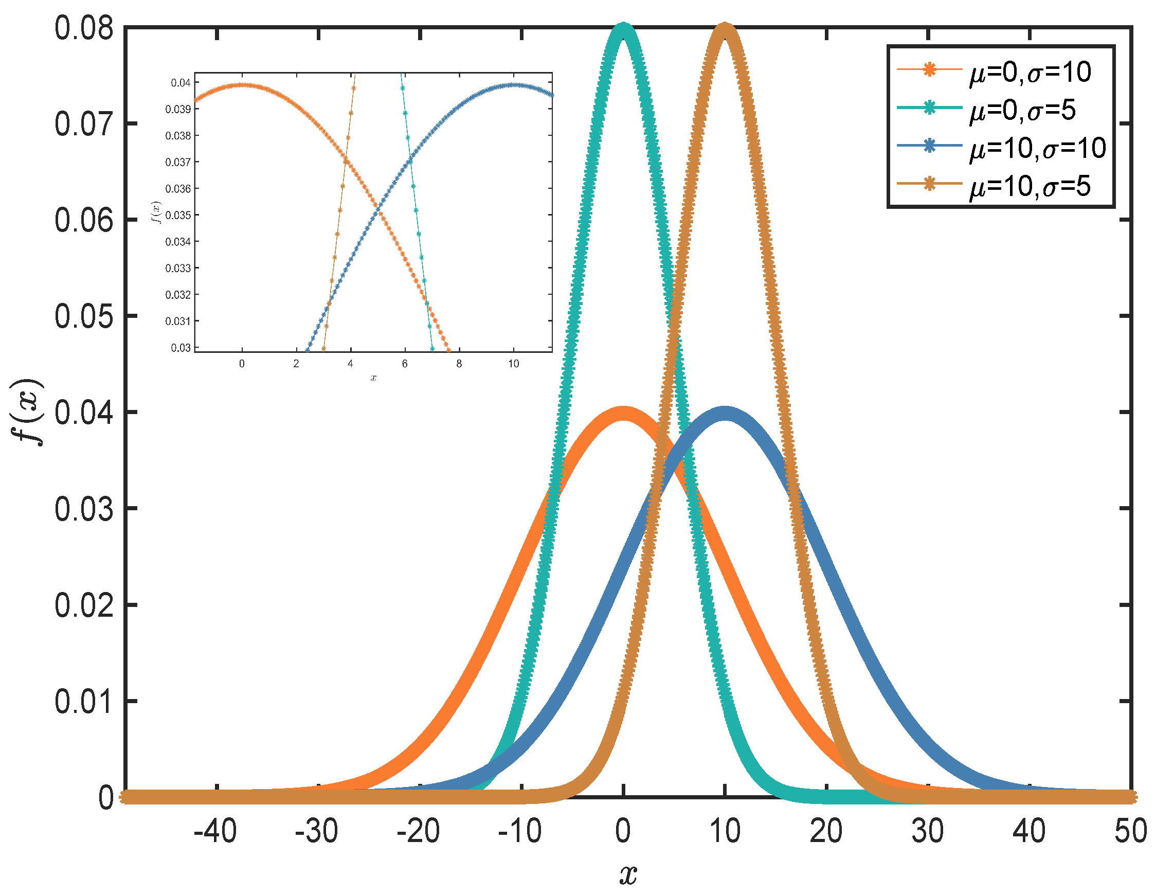
Figure 1. Figure of probability density function of normal distribution.
Energies 16 05466 g001
Figure 2. Plot of β in GSCE and CE.
Energies 16 05466 g002
Figure 3. Plot of chaotic sequence of Logistic map.
Energies 16 05466 g003
Figure 4. Structure of variables existing in calculation of total constraints violation.
Energies 16 05466 g004
Figure 5. Process of calculation of normalized constraints violation.
Energies 16 05466 g005
Figure 6. One line diagram of IEEE-30 bus system.
Energies 16 05466 g006
Figure 7. Fuel cost considering multi-fuels.
Energies 16 05466 g007
Figure 8. Box plot of three CE methods in Case 1 and Case 2. (a) Case 1, (b) Case 2. The red bold + specify the outliers.
Energies 16 05466 g008
Figure 9. One line diagram of IEEE-57 bus system.
Energies 16 05466 g009
Figure 10. Voltage profile provided by CGSCE in Case 7.
Energies 16 05466 g010
Figure 11. The convergence comparison of three CE methods. (a) Case 1, (b) Case 2, (c) Case 4, (d) Case 5, (e) Case 6, (f) Case 7.
Energies 16 05466 g011
Figure 12. Comparison of CE method with different β in Case 1.
Energies 16 05466 g012
Table 1. Summary of study cases for IEEE-30 bus system.
Study CaseBasic Fuel CostMulti-Fuel OptionL-IndexEmissionPower Loss
Case 1
Case 2
Case 3
Case 4
Case 5
Table 2. Parameters setting of three CE method for IEEE-30 bus system.
AlgorithmPopulation SizeNumber of Elites α β q
CGSCE10010-0.95
GSCE10010---
CE100100.80.95
Table 3. Simulation results of CGSCE, GSCE and CE for IEEE-30 bus system.
StudyCGSCE GSCE CE
CaseMinAvgMaxMinAvgMaxMinAvgMax
Case 1800.5106800.5118800.5150800.5109800.5214800.5416800.5154800.5196800.5353
Case 2646.5803650.8642667.2889646.6502660.6629726.0109646.7323657.4860725.7435
Case 30.136670.137130.137550.137010.137640.138240.136570.137160.13775
Case 40.2048230.2048310.2048540.2048230.2048440.204870.2048230.2048240.204824
Case 53.100603.107273.173113.101173.134343.202553.101503.107193.14864
The results in bold type specify the best solutions.
Table 4. Standard deviation and simulation time of CGSCE, GSCE and CE for IEEE-30 bus system.
StudyCGSCE GSCE CE
CaseStdSimulation Time (s)StdSimulation Time (s)StdSimulation Time (s)
Case 10.00097881.430.00766577.590.00203377.69
Case 29.18923079.6849.23406078.7726.99508976.75
Case 30.00039780.070.00030278.520.00034178.86
Case 4 9.276 × 10 06 76.30 1.434 × 10 06 77.33 2.401 × 10 07 74.57
Case 50.01801377.890.03282579.160.00133478.07
Table 5. Simulation results of the best solutions of three CE methods in Case 1 to Case 3.
ParameterMinMax CGSCE GSCE CE
Case 1Case 2Case 3Case 1Case 2Case 3Case 1Case 2Case 3
P G 2 M W 208048.693154.998766.736948.689855.000041.529348.881554.972752.1764
P G 5 M W 155021.370824.116037.378621.384924.0185040.387621.351523.658144.2338
P G 8 M W 103521.272034.982027.594721.268734.890227.150221.195634.784533.1755
P G 11 M W 103011.970818.670718.435111.946018.885017.277711.944618.826528.6691
P G 13 M W 124012.001117.393527.816212.000017.384613.375712.010717.954517.5278
V 1 ( p . u . ) 0.951.11.08481.07521.05721.08451.07251.08061.08451.07481.0545
V 2 ( p . u . ) 0.951.11.06531.05931.05201.06501.05711.06231.06511.05951.0474
V 5 ( p . u . ) 0.951.11.03381.03031.06461.03361.02811.06751.03371.03301.0644
V 8 ( p . u . ) 0.951.11.03841.03881.04451.03831.03771.03211.03831.04171.0524
V 11 ( p . u . ) 0.951.11.09931.08901.09991.09691.06511.08001.08581.06851.0977
V 13 ( p . u . ) 0.951.11.04621.06131.08631.04641.07751.07601.04841.04911.0894
Q C 10 ( M W ) 051.58963.94451.46900.42963.96260.42214.22224.54802.1011
Q C 12 ( M W ) 051.12632.23502.19542.31800.17550.05530.92072.16591.7148
Q C 15 ( M W ) 054.23013.34830.67513.72874.14270.79244.28124.15040.0000
Q C 17 ( M W ) 054.97193.82432.17314.99894.05451.56824.96873.68050.3894
Q C 20 ( M W ) 054.02184.07513.08474.01963.94963.07963.76565.00001.3733
Q C 21 ( M W ) 054.99724.15470.00234.99823.88810.09714.95733.70020.3308
Q C 23 ( M W ) 052.91414.27290.00733.06513.88671.41342.92483.50280.0112
Q C 24 ( M W ) 055.00003.51210.01455.00004.99750.11294.98124.62110.0000
Q C 29 ( M W ) 052.47533.04790.01402.42031.05450.00442.31903.79930.0644
T 11 ( p . u . ) 0.91.11.03771.01451.03521.06541.00341.00651.05201.04061.0415
T 12 ( p . u . ) 0.91.10.95390.98650.90020.91620.95350.90010.93900.94790.9036
T 15 ( p . u . ) 0.91.10.96870.99681.03670.97131.02421.00290.97100.99811.0308
T 36 ( p . u . ) 0.91.10.97410.97800.95500.97370.96440.94900.97540.98690.9594
P G 1 ( M W ) 50200177.1200139.9995111.3297177.1394140.0000150.7777177.0473139.9892112.9882
Q G 1 ( M V A r ) −201506.56713.2187−19.36366.30580.55957.93956.31231.8150−18.0799
Q G 2 ( M V A r ) −206025.421716.7715−4.220625.121216.51314.937425.199816.3314−13.9467
Q G 5 ( M V A r ) −1562.527.570226.327160.137427.701226.569560.767027.720628.621358.0778
Q G 8 ( M V A r ) −1548.729.229825.993935.922829.677430.877722.596029.611731.490647.1502
Q G 11 ( M V A r ) −104027.193220.902926.708029.71549.295515.841423.692717.026626.9806
Q G 13 ( M V A r ) −1544.7−2.73329.213128.6934−2.598121.401520.0612−1.07515.147930.8721
Fuel cost ($/h) 800.5106646.5803851.1982800.5109646.6502830.2833800.5141646.7323863.1420
Emission(t/h) 0.3661950.2835110.2432750.3662530.2834750.3006480.3660330.2833710.241214
P l o s s ( M W ) 9.027766.760425.891369.028886.778297.098409.031146.785415.37070
V D ( p . u . ) 0.916610.869970.882450.908230.912710.862970.890050.778690.87184
L i n d e x ( m a x ) 0.138090.138860.136670.138090.137810.137010.138570.140180.13657
The results in bold type specify the best solutions.
Table 6. Simulation results of the best solutions of three CE methods in Case 4 and Case 5.
ParameterMinMaxCGSCE GSCE CE
Case 4Case 5Case 4Case 5Case 4Case 5
P G 2 M W 208067.576279.999767.573780.000067.592679.9843
P G 5 M W 155050.000050.000050.000050.000049.999949.9996
P G 8 M W 103535.000034.999935.000035.000035.000035.0000
P G 11 M W 103030.000030.000030.000030.000030.000029.9999
P G 13 M W 124040.000040.000040.000039.999340.000040.0000
V 1 ( p . u . ) 0.951.11.06291.06211.06281.06171.06351.0621
V 2 ( p . u . ) 0.951.11.05681.05791.05661.05751.05751.0577
V 5 ( p . u . ) 0.951.11.03741.03851.03721.03791.03701.0384
V 8 ( p . u . ) 0.951.11.04381.04481.04361.04421.04431.0445
V 11 ( p . u . ) 0.951.11.07871.07911.08301.07831.07941.0887
V 13 ( p . u . ) 0.951.11.05941.05581.06211.05611.05301.0573
Q C 10 ( M W ) 051.33672.12450.27672.65593.07460.3799
Q C 12 ( M W ) 051.51712.14900.42633.49143.64230.8590
Q C 15 ( M W ) 054.22714.25333.73704.30114.10174.5878
Q C 17 ( M W ) 054.98534.99644.99934.99944.82664.8344
Q C 20 ( M W ) 053.87463.94173.98393.86213.71853.9194
Q C 21 ( M W ) 054.99735.00005.00005.00004.92785.0000
Q C 23 ( M W ) 052.91172.91683.20872.99683.07252.9412
Q C 24 ( M W ) 054.99924.99924.99965.00004.96624.9682
Q C 29 ( M W ) 052.33532.39962.36062.37412.05452.2758
T 11 ( p . u . ) 0.91.11.07081.08241.04691.05351.05681.0672
T 12 ( p . u . ) 0.91.10.90660.90170.93030.92980.92700.9183
T 15 ( p . u . ) 0.91.11.00000.99561.00130.99990.99430.9954
T 36 ( p . u . ) 0.91.10.97620.97720.97640.97670.97520.9774
P G 1 M W 5020064.058651.501064.061651.502064.043451.5177
Q G 1 ( M W ) −20150−2.0884−2.1765−2.1445−2.5592−1.8719−1.9032
Q G 2 ( M W ) −206012.152412.000212.107411.877113.712511.4035
Q G 5 ( M W ) −1562.523.859923.942623.839723.757622.881823.9256
Q G 8 ( M W ) −1548.729.625829.757729.382329.261230.083228.9347
Q C 11 ( M W ) −104023.703425.145722.534521.319322.154327.2559
Q C 13 ( M W ) −1544.78.13765.381310.18625.59533.31506.5615
Fuel cost ($/h) 944.3944967.663944.3917967.6631944.4232967.6297
Emission(t/h) 0.2048230.2072670.2048230.2072670.2048230.207261
(MW) 3.234713.100603.235253.101173.235813.10150
VD (p.u.) 0.888080.890960.893380.897450.893140.89192
L-index(max) 0.138590.138570.138580.138560.138560.13861
The results in bold type specify the best solutions.
Table 7. Comparison of the best results for Case 1.
AlgorithmFuel CostEmissionPower LossVoltage DeviationL-Index
CGSCE800.51060.3660339.031140.890050.13857
GSCE800.51090.3662539.028880.908320.13809
CE800.51540.366639.03840.905250.13829
MSFLA [12]802.2870.3723---
SFLA [12]802.50920.372---
Hybrid MPSO-SFLA [13]801.750.3779.54--
ABC [15]800.660.3651419.03280.92090.1381
TLBO [17]801.99080.3668---
MTLBO [17]801.89250.3665---
ARCBBO [19]800.51590.36630.88670.1385
MICA-TLA [14]801.04880.36669.1895--
AGSO [45]801.750.3703---
SMA [46]802.54490.3635529.5232--
The result in bold type specify the best solution.
Table 8. Comparison of the best results for Case 2.
AlgorithmFuel CostEmissionPower LossVoltage DeviationL-Index
CGSCE646.58030.2835116.760420.869970.13886
GSCE646.65020.2834756.778290.912710.13781
CE646.73230.2833716.785410.778690.14018
DE [1]650.82240.28317.63330.57330.1366
SFLA [12]654.470.2902---
Hybrid MPSO-SFLA [13]647.550.2834---
ABC [15]649.08550.2825637.25260.66650.1383
GABC [16]647.030.28356.8160.801-
TLBO [47]647.9202-7.10641.41730.1211
LTLBO [18]647.43150.28356.93470.8896-
MICA-TLA [14]647.10020.28356.8945--
MSA [36]646.83640.283526.80010.844790.13867
The result in bold type specify the best solution.
Table 9. Comparison of the best results for Case 3.
AlgorithmL-IndexFuel CostEmissionVoltage DeviationPower Loss
CGSCE0.13667851.19820.2432750.882455.89136
GSCE0.13701830.28330.3006480.862977.09840
CE0.13657863.1420.2412140.871845.37070
ABC [15]0.1379801.6650.3642950.9389.2954
MICA-TLA [14]0.1369801.80760.36280.85219.229
SF-DE [20]0.13671875.89290.228010.903874.6412
The result in bold type specify the best solution.
Table 10. Comparison of the best results for Case 4.
AlgorithmEmissionFuel CostPower LossVoltage DeviationL-Index
CGSCE0.204823944.39443.234710.888080.13859
GSCE0.204823944.39173.235250.893380.13858
CE0.204823944.42323.235810.893140.13856
SFLA [12]0.2063951.5106---
MSFLA [12]0.2056960.1911---
Hybrid MPSO-SFLA [13]0.2052----
GSO [45]0.206954.9512---
AGSO [45]0.2059953.629---
DSA [48]0.2058255944.40863.24373-0.12734
MSA [36]0.20482944.50033.23580.873930.13888
SF-DE [20]0.20482944.32423.21790.896170.13844
The result in bold type specify the best solution.
Table 11. Comparison of the best results for Case 5.
AlgorithmPower LossFuel CostEmissionVoltage DeviationL-Index
CGSCE3.10060967.66300.2072670.890960.13857
GSCE3.10117967.66310.2072670.897450.13856
CE3.10150967.62970.2072610.891920.13861
EGA [49]3.2008967.86--0.12178
ABC [15]3.1078967.6810.2072680.90080.1386
EEA [50]3.2823952.37850.206735-0.1533
TLBO [51]3.11389967.49149--0.12651
The result in bold type specify the best solution.
Table 12. Simulation result of CGSCE, GSCE and CE for IEEE-57 bus system.
StudyCGSCE GSCE CE
CaseMinAvgMaxMinAvgMaxMinAvgMax
Case 641,667.277741,700.472241,765.47741,683.569541,718.795441,830.228841,669.022241,681.033741,696.1114
Case 70.58800.60550.63220.59780.62590.67310.59270.60140.6238
The results in bold type specify the best solutions.
Table 13. Standard deviation and simulation time of CGSCE, GSCE and CE for IEEE-57 bus system.
StudyCGSCE GSCE CE
CaseStdSimulation Time (s)StdSimulation Time (s)StdSimulation Time (s)
Case 631.301284126.0930.840003128.718.274621128.82
Case 70.012038129.750.020917129.310.006462129.73
Table 14. Simulation results of the best solutions of three CE methods in Case 6 and Case 7.
ParameterMinMaxCGSCE GSCE CE
Case 6Case 7Case 6Case 7Case 6Case 7
P G 2 M W 3010090.655135.031088.469772.955688.244951.1308
P G 3 M W 4014045.0428112.064745.061482.774744.611364.7434
P G 6 M W 3010071.705830.108272.981146.475673.462832.4851
P G 8 M W 100550460.4218295.5435460.2346259.9944458.7908277.3415
P G 9 M W 3010094.945999.985995.672099.999996.807897.2581
P G 12 M W 100410360.1364297.4539360.9547375.5547360.266341.5521
V 1 ( p . u . ) 0.951.11.06581.01101.03431.01901.05881.0119
V 2 ( p . u . ) 0.951.11.06351.00841.03301.01751.05681.0082
V 3 ( p . u . ) 0.951.11.05551.01521.02941.01761.05201.0101
V 6 ( p . u . ) 0.951.11.06231.00171.04530.99971.05931.0038
V 8 ( p . u . ) 0.951.11.07251.01971.05801.00781.07431.0252
V 9 ( p . u . ) 0.951.11.04601.00701.02650.99941.04681.0122
V 12 ( p . u . ) 0.951.11.04481.01341.02141.02651.04591.0383
Q C 18 ( M W ) 0209.40155.954611.867216.72086.30641.6996
Q C 25 ( M W ) 02014.032919.409215.623616.952714.972119.7239
Q C 53 ( M W ) 02012.653519.999912.995920.000012.778220.0000
T 19 ( p . u . ) 0.91.10.97841.07620.92930.98180.97680.9395
T 20 ( p . u . ) 0.91.11.00060.94761.01291.07001.00001.0137
T 31 ( p . u . ) 0.91.11.00940.96891.01120.97161.00700.9722
T 35 ( p . u . ) 0.91.11.07391.07101.09081.09771.03101.0650
T 36 ( p . u . ) 0.91.10.96301.05760.96810.98891.03711.0610
T 37 ( p . u . ) 0.91.11.02811.00381.02520.99921.02861.0056
T 41 ( p . u . ) 0.91.10.99620.99410.98290.98480.99710.9959
T 46 ( p . u . ) 0.91.10.96130.91900.96430.91790.96290.9211
T 54 ( p . u . ) 0.91.10.90830.90000.90000.90000.90560.9009
T 58 ( p . u . ) 0.91.10.97890.92960.95390.93030.97860.9309
T 59 ( p . u . ) 0.91.10.96330.98120.94000.96740.96320.9902
T 65 ( p . u . ) 0.91.10.97031.00110.94941.00280.97131.0090
T 66 ( p . u . ) 0.91.10.93480.90000.91300.90000.93210.9000
T 71 ( p . u . ) 0.91.10.96970.95680.94760.95990.98010.9648
T 73 ( p . u . ) 0.91.10.99471.00880.99380.98860.99801.0064
T 76 ( p . u . ) 0.91.10.96720.90010.96760.90260.96210.9014
T 80 ( p . u . ) 0.91.10.99280.98800.97090.98120.99780.9954
P G 1 ( M W ) 0576142.7851404.2220142.6836331.5767143.5011409.7128
Q G 1 ( M V A r ) −14020052.0709−30.448136.8008−8.235840.0044−32.0001
Q G 2 ( M V A r ) −175049.995049.808149.999349.998648.366347.4032
Q G 3 ( M V A r ) −106032.655159.985730.465658.527337.533656.6139
Q G 6 ( M V A r ) −825−0.2248−7.89373.5300−7.8941−5.2681−5.5796
Q G 8 ( M V A r ) −14020046.627642.439358.478028.154054.680350.5760
Q G 9 ( M V A r ) −398.99948.99839.00008.99978.18778.9706
Q G 12 ( M V A r ) −15015546.8299154.437951.7570117.225056.6570152.5423
Fuel cost ($/h) 41,667.277749,522.928341,683.569546,244.204341,669.022248,776.4802
Emission(t/h) 1.9207681.6166551.9210511.4683871.9040561.703746
P l o s s ( M W ) 14.8929123.6091515.2570518.5315914.8846923.42392
V D ( p . u . ) 1.695900.588031.457950.597781.566970.59268
L i n d e x ( m a x ) 0.279160.301380.281630.300630.282330.30072
The results in bold type specify the best solutions.
Table 15. Comparison of the best results for Case 6.
AlgorithmFuel CostEmissionPower LossVoltage DeviationL-Index
CGSCE41,667.27771.92076814.892911.695900.27916
GSCE41,683.56951.92105115.257051.457950.28163
CE41,669.02221.90405614.884691.566970.28233
ABC [15]41,693.9589----
GSA [53]41,695.8717----
ARCBBO [19]41,686-15.3769--
MO-DEA [54]41,683 15.27271.50330.2816
KHA [55]41,709.2647--1.68930.2733
TLBO [18]41,695.66261.98048815.7469--
LTLBO [18]41,679.54511.93067615.1589--
DSA [48]41,686.82--1.0832670.24353
ICBO [37]41,697.33241.91790315.5471.31730.2776
MSA [36]41,673.721.952615.05261.55080.28392
The result in bold type specify the best solution.
Table 16. Comparison of the best results for Case 7.
AlgorithmVoltage DeviationFuel CostEmissionPower LossL-Index
CGSCE0.5880349,522.92831.61665523.609150.30138
GSCE0.5977846,244.20431.46838718.531590.30063
CE0.5926848,776.48021.70374623.423920.30072
APFPA [56]0.890943,485.933-12.1513-
SP-DE [20]0.5926745,549.491.289818.42750.30052
SF-DE [20]0.5958445,246.021.2345318.46970.30135
ESCHT-DE [20]0.6041646,813.221.337919.08210.3008
The result in bold type specify the best solution.
Disclaimer/Publisher’s Note: The statements, opinions and data contained in all publications are solely those of the individual author(s) and contributor(s) and not of MDPI and/or the editor(s). MDPI and/or the editor(s) disclaim responsibility for any injury to people or property resulting from any ideas, methods, instructions or products referred to in the content.