Research on Product Yield Prediction and Benefit of Tuning Diesel Hydrogenation Conversion Device Based on Data-Driven System

Abstract

In the refining process, a large amount of data are generated in daily production, and how to make full use of these data to improve the accuracy of simulation is the key to improving the operation level of refineries. At the same time, with the increasing environmental regulations and the improvement of gasoline and diesel quality standards, the ratio of diesel to gasoline is also changing with people’s demand for fuel consumption. Catalytic cracking light cycle oil (LCO) hydrogenation conversion technology (react LCO into gasoline, RLG) can produce modified diesel with high-octane gasoline, a high cetane number, and a low sulfur content, which improves the added value of the product. In this article, based on the production and operation data of a 1 million tons/year RLG device, a device yield prediction model was established using a deep neural network (DNN) algorithm, and the model was further optimized using a genetic algorithm (GA) to maximize the economic benefits of the device. As a result, the gasoline production yield increased by more than 3%. The experimental results show that the established model has a good reference value for improving the economic benefits of the RLG device.

1. Introduction

The hydrocracking unit for catalytic diesel (LCO) in the refining plant converts low-quality LCO with a high density, high aromatic hydrocarbon content, and low cetane number into high-octane gasoline, liquefied petroleum gas, and high-cetane diesel. Through this process, the added value of the product can be increased, with better economic and social benefits. The reaction process of RLG involves a hydrorefining reaction and hydrocracking reaction, which include complex chemical reactions in the reaction system. It is difficult to establish a model to simulate the actual reaction process. In previous studies, researchers have developed different types of models to simulate and optimize the refining process, which can be categorized into two main categories.

The first is the mechanism-driven model (MDM), also known as the summation model, which is based on a number of assumptions and reaction mechanisms to model the actual reaction process [1]. The three main types of MDMs are wide fraction summation, narrow fraction summation, and continuous summation. At present, the mainstream direction of MDM research in hydrocracking reactor modeling still focuses on narrow fraction integration model research, and the research on the narrow fraction integration model is primarily based on the Chevron model proposed by Stangeland [2]. The most significant feature of the Chevron model is that Stangeland considers both the feedstock and product as compounds with continuous distillation curves. The physical and chemical properties displayed by the compounds during cracking largely depend on the difference in real boiling points [3]. He divided these raw materials and products into various lumps every 50°F from the initial boiling point [2]. By performing this, he obtained multiple components with distinct properties, which were used to construct a narrow lumped model. Being the first model to apply the total theory of narrow fractionation to the hydrocracking process, it pioneered the development of the prototype reaction rate equation and achieved the objective of optimizing the increase in aero coal production through the model. Subsequently, Mohanty et al. proposed the introduction of a system of heat equations to calculate the temperature distribution in the catalytic bed of a reactor [4]. Pacheco and others used the Chevron model as the foundation for their endeavors to refine the chemical reaction equilibrium [5]. However, MDM is based on numerous assumptions to simplify complex processes in actual production. They are also limited by the coupling effects between operational conditions, leading to a relatively lower accuracy. Therefore, their usage is subject to limitations [1,6].

The second category is the data-driven model (DDM), which is also known as a black box model [1]. The main characteristic of the DDM model is that it is based on existing operational data to establish the mapping relationship from inputs to outputs. This helps to avoid strong coupling between process conditions, thereby improving prediction accuracy [7]. Chen and his colleagues adopted artificial neural networks (ANNs) to learn the sum of manipulative variables, such as pallet temperature, for optimizing ANN models [8]. Meanwhile, Song and his colleagues used polynomial models to model production and industrial processes [7].

Therefore, there is an urgent need to develop a reliable DDM to guide actual production. In this paper, an RLG device yield prediction model was established based on a DNN algorithm, and then the RLG device yield model was established by a GA, which provides a guiding direction for RLG device yield prediction and benefit adjustment.

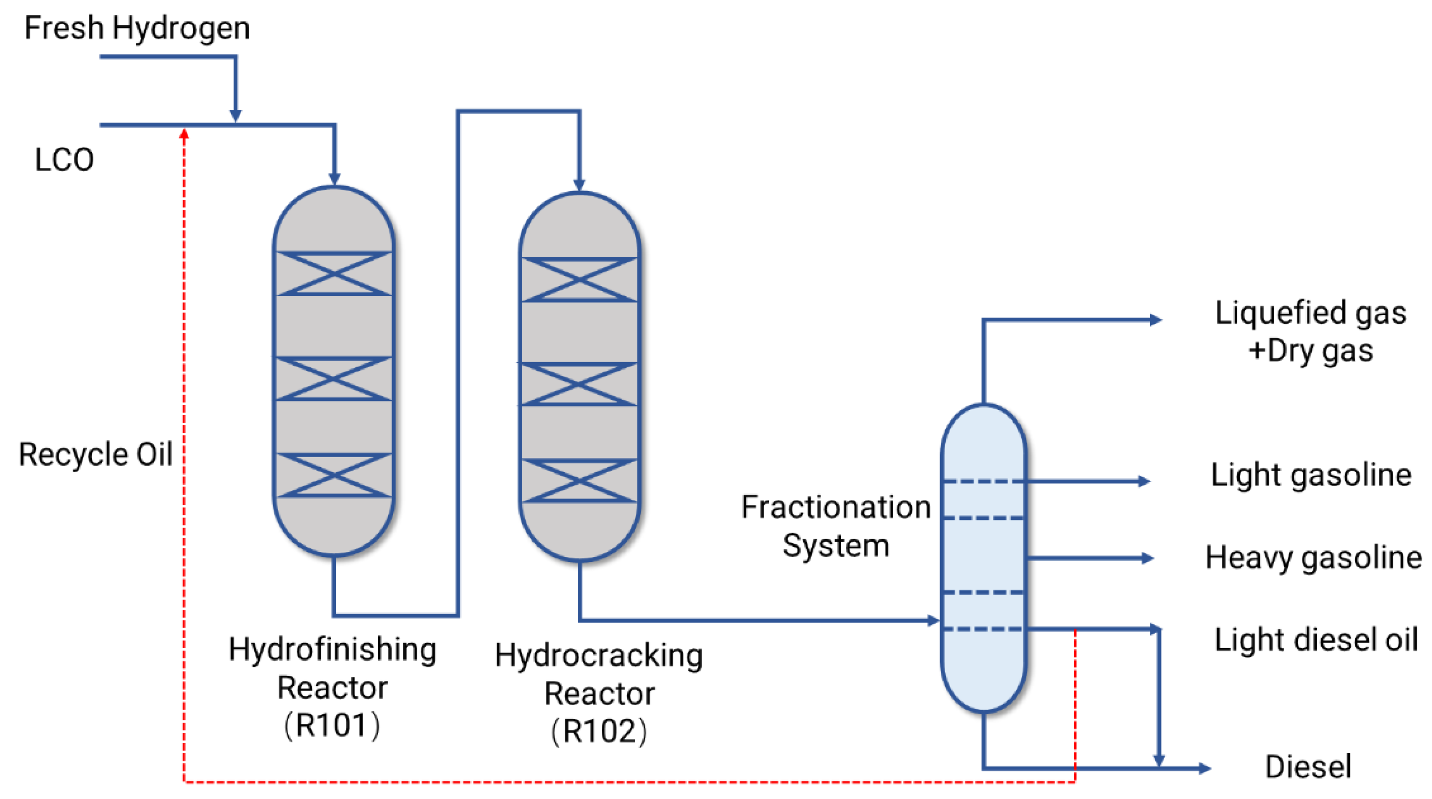
2. Industrial Hydrocracking Process

A simplified flow diagram of a typical RLG process is shown in Figure 1. The feedstock for an RLG device is LCO from an FCC device. The new feed is mixed with externally generated supplementary hydrogen and heated to a specified temperature before entering the reactor. The RLG device consists of two tandem reactors. The first reactor is primarily loaded with a hydrofinishing catalyst, which is used to remove a significant portion of the sulfur, nitrogen, and other heavy metal compounds present in the feedstock. The second reactor, on the other hand, is equipped with a hydrocracking catalyst, where most of the cracking reactions occur. After the second reactor, a high-pressure separator (HPS) recovers unreacted hydrogen from the reactor effluent and then a low-pressure separator (LPS) separates some of the lighter gases from the HPS effluent. Finally, the different products are separated in the fractionation section.

3. Experimental Methods

3.1. Overall Framework

The first step in the proposed model is to collect plant data from the refinery, including feedstock characteristics, operating conditions, and product yields [8]. The data are then preprocessed, including outlier removal, data transformation, and normalization. After that, the dataset is divided into training samples and testing samples. Next, a suitable DNN model structure is designed. Based on this, the input variables are mapped into a two-dimensional representation to extract process features. The model is then constructed and trained. Finally, based on the established DNN model, a data-driven model of RLG device revenue optimization is constructed, and the model is solved using an intelligent optimization algorithm to obtain the optimal combination of process parameters. This can guide the actual production process of the factory.

3.2. Deep Nerual Network

DNNs are the foundation of machine learning, also known as multi-layer perceptron (MLP) [9], derived from the early shallow ANN model. The layered network structure formed by artificial neurons constitutes the basic model structure of DNNs. A standard DNN model consists of an input layer, several hidden layers, and an output layer, with the structure between the input layer and the output layer collectively referred to as the hidden layers. Compared with the shallow ANN model, the DNN model has a larger number of hidden layers, and the large number of hidden layers means DNN’s “depth”, so the DNN has stronger modeling capabilities for complex nonlinear systems [10].

3.3. Data Collection and Preprocessing

In this paper, the DCS system using the RLG device collected data from the operation of the device from June 2018 to July 2021. During the data collection process, there can be various flaws in the collected data due to device maintenance, faults in the data collection system, or human errors. These flaws can include data duplication, incompleteness, inaccuracies, and other defects. Data preprocessing is an integral part of data mining, ensuring the accuracy and effectiveness of the data, thereby enhancing the efficiency of data mining. If the error in the data is not preprocessed and eliminated before modeling, the selection of subsequent related variables and the calculation of time delay will be affected, and the final model may not achieve the prediction function or the prediction effect may be poor, thus losing the guiding significance for actual production.

The input variables considered in the dataset include 8 operational variables and 9 physical variables, and the output variables include 4 product yields. The statistics of the dataset are summarized in

Table 1. Statistics of dataset.

Category	Number	Definition
inputs	17	(1) Fresh diesel feed, new hydrogen, the earliest distilled light oil fraction volume, amount of pre-hydrogenated sulfur-containing light hydrocarbons in the take-up reformer, feedstock density (20 °C), feedstock total sulfur content, feedstock total nitrogen content, and 95% distillation temperature of feedstock. (2) R101 average temperature, R101 inlet hydrogen partial pressure, R101 inlet circulating hydrogen volume, R101 inlet hydrogen–oil ratio, R102 average temperature, R102 inlet hydrogen partial pressure, R102 inlet circulating hydrogen volume, R102 inlet hydrogen–oil ratio, R102 inlet hydrogen–oil ratio, actual circulating hydrogen purity,
outputs	5	gasoline yield, diesel yield, LPG yield, dry gas yield. R102 temperature rise

below.

In order to eliminate dimensional differences between different variables and the masking effect of large numbers on small numbers, based on the data collected by the RLG device, it is necessary to standardize the data before further analysis and modeling. Since the z-score standardization method maps the data to a standard normal distribution, It is beneficial for the subsequent training and convergence of neural network models. After saving the mean and variance of the current data, future new data can be directly standardized. Therefore, the z-score normalization method was selected to transform the sample data, and the calculation is as shown in Equation (1).

$$X_{Norm}=\frac{X-\mu }{\sigma }$$

(1)

Before establishing the prediction model of the DNN, the sample data need to be divided into a training set and testing set, where the training set is used for model training, and the testing set is used for model generalization ability evaluation. This paper divided 974 sets of samples into 779 groups of training sets and 195 groups of testing sets according to the ratio of training set: testing set = 8:2.

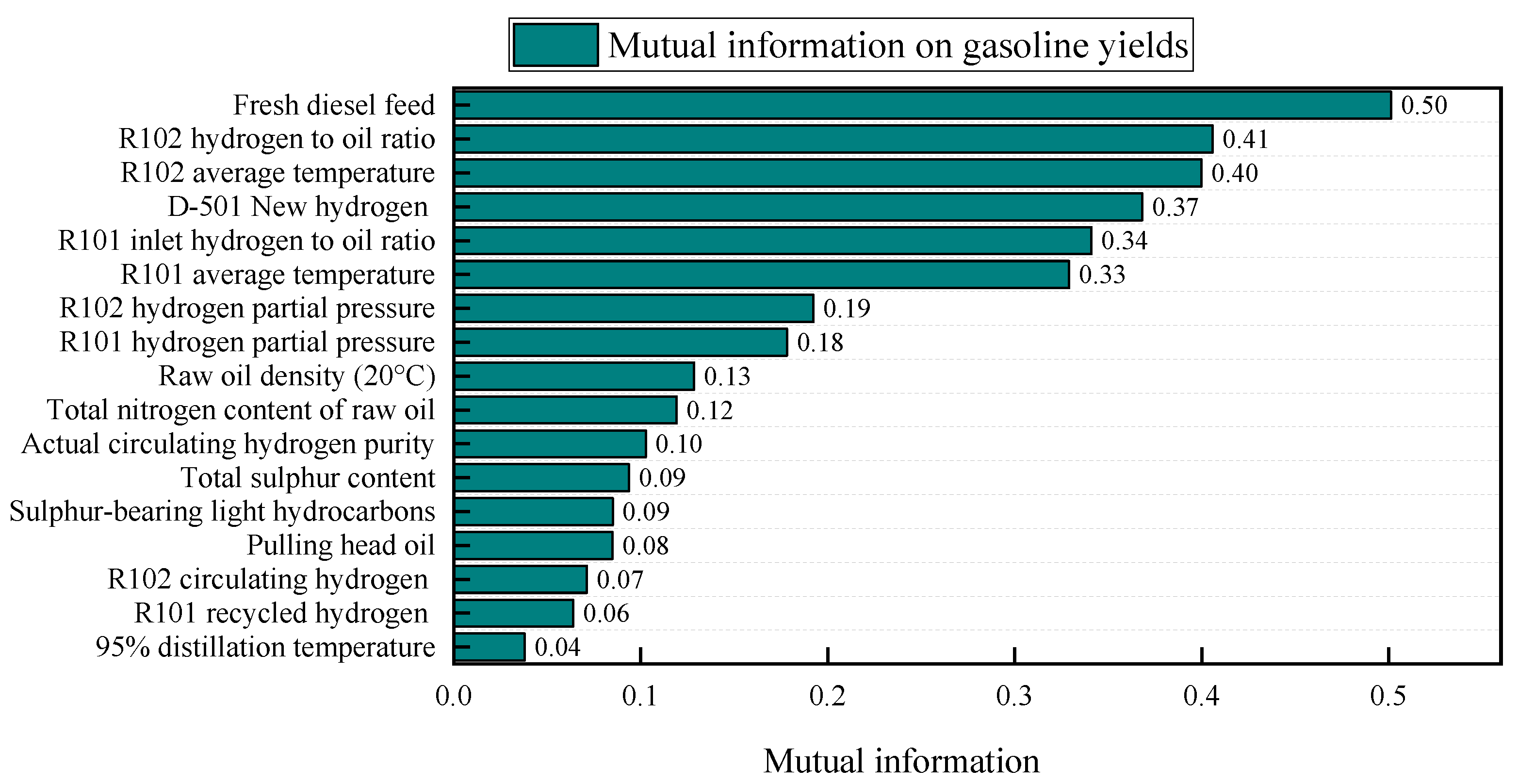
3.4. Analysis and Selection of Modeling Variables

By calculating the correlation between each input variable of the model and the prediction target, we can measure the contribution of different input variables to the predicted target. This allows us to quantify the influence of physical property variables and process parameters on product distribution in actual production. Mutual information is a measure that quantifies the linear or nonlinear correlation between two variables [11,12]. It is also used to characterize the amount of information that one random variable contains about another random variable. This is because knowing the value of one variable can reduce the uncertainty or increase the predictability of the other variable. Mutual information can be calculated using Equation (2). This section calculates the mutual information between the input variables and the five prediction targets of gasoline yield, diesel yield, liquefied gas yield, dry gas yield, and R102 temperature rise. The greater the mutual information, the greater the contribution of the input variables to the prediction target. Take gasoline yield as an example, as shown in Figure 2.

$$I(X,Y)={\displaystyle \sum _{X,Y}p(X,Y)\cdot \log [\frac{p(X,Y)}{p(X)\cdot p(Y)}]}$$

(2)

where p(X, Y) is the joint probability of variables X and Y, and p(X) and p(Y) are the marginal probabilities of variables X and Y, respectively.

Figure 2 shows the mutual information between the model input variables and gasoline yield. It reveals that fresh diesel feed has the greatest impact on gasoline yield, followed by the inlet hydrogen-to-oil ratio (R102) and average temperature, which also have substantial effects on gasoline yield. These impacts are higher than those of the inlet hydrogen-to-oil ratio and average temperature of R101. This can be attributed to the underlying principle of the RLG process, where different types of reactions occur in the two reactors. R101 is a refining reactor primarily involved in desulfurization and denitrification reactions, while R102 is a cracking reactor involved in opening and cracking reactions. The latter has a more direct impact on gasoline yield. Therefore, the results of the mutual information analysis align with the actual process. In addition, the D-501 new hydrogen gas flow rate, R101 inlet hydrogen partial pressure, and R102 inlet hydrogen partial pressure also significantly influence gasoline yield. These three variables primarily affect the hydrogen mixing flow rate, which, in turn, affects the depth of hydrogenation reactions in R101 and R102, ultimately impacting gasoline production. The remaining variables exhibit similar mutual information to the gasoline yield, but to a lesser extent than the aforementioned variables.

3.5. Genetic Algorithm

The GA is an algorithm that draws on the natural law of superiority and inferiority in reproduction [13]. It was developed primarily by mimicking biological evolutionary mechanisms in nature, a phenomenon that we call genetics. The core operation of the GA is a random search algorithm using genetic models: the optimization problem is mapped to a genetic space, where various potential solutions are encoded as chromosomes. Each chromosome represents a solution, and each bit on the chromosome is called a gene, which is represented by a binary string [14]. The mathematical model of RLG device revenue optimization is a non-linear optimization problem with constraints, which can be solved using intelligent optimization algorithms. Commonly used intelligent optimization algorithms include particle swarm algorithms (PSOs) [15], GAs, simulated annealing algorithms (SAs) [16], and ant colony algorithms (ACOs) [17], among which genetic algorithms are more widely used in the petrochemical industry and have good applicability to different tasks, so they were chosen as the optimization algorithm in this study.

4. Results and Discussion

4.1. RLG Device Yield Prediction Model

4.1.1. Selection of DNN Model Parameters

(1)

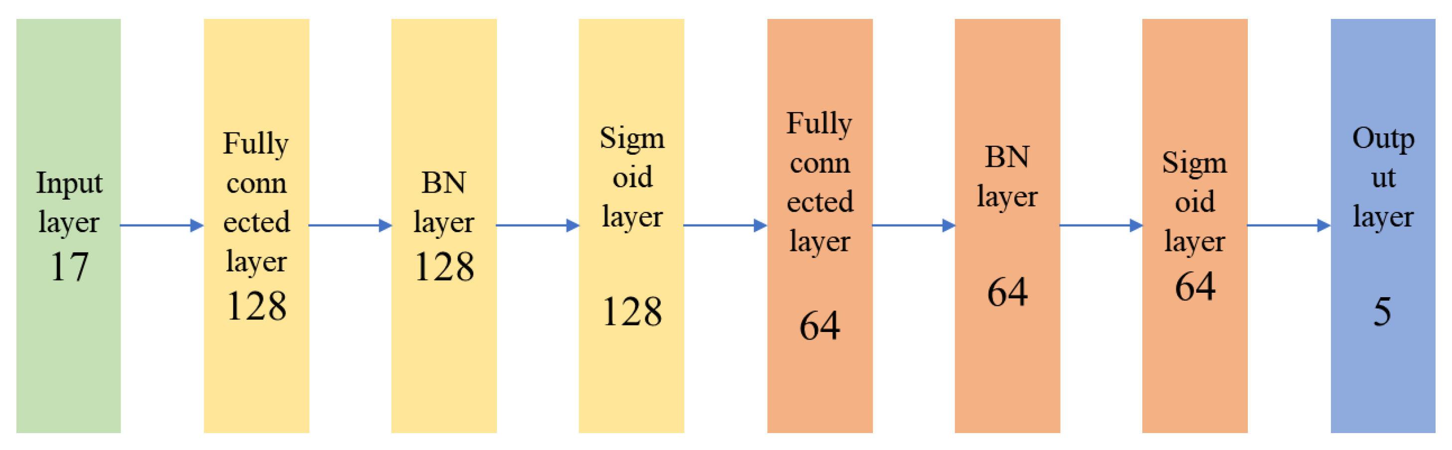
Establishment of input and output neuron layers

The analysis established that there were 17 input variables in the input layer, divided into 2 categories, as shown in

Table 2. Variables of DNN model.

Program	Number of Variables	Variable Name
Input variables	17	(1) Fresh diesel feed volume, D-501 fresh hydrogen inlet flow rate, the earliest distilled light oil fraction volume, amount of sulfur-containing light hydrocarbons in the pre-hydrogenation of the collected reformer, feedstock density (20 °C), feedstock total sulfur content, feedstock total nitrogen content, and 95% distillation temperature of the feedstock; (2) R101 average temperature, R101 inlet hydrogen partial pressure, R101 inlet circulating hydrogen volume, R101 inlet hydrogen–oil ratio, R102 average temperature, R102 inlet hydrogen partial pressure, R102 inlet circulating hydrogen volume, R102 inlet hydrogen–oil ratio, R102 inlet hydrogen–oil ratio Actual circulating hydrogen purity
Output variables	5	Gasoline yield, diesel yield, LPG yield, dry gas yield; R102 temperature rise

; and that there were 5 output variables in the output layer, which were the 4 main product yields of the RLG device and a di-inverse temperature rise: gasoline yield, diesel yield, LPG yield, dry gas yield, and R102 temperature rise. The selection of the number of hidden layers and neurons typically requires empirical judgment. Thus, the optimal number of hidden layers and neuron nodes needs to be determined by analyzing and comparing the prediction results of testing sets corresponding to different numbers of hidden layers.

(2)

Batch_Size

Batch_Size refers to the number of samples used for training in each batch when the model is trained on the data in batches [18]. Setting Batch_Size appropriately can avoid large prediction fluctuations and achieve better convergence. When setting Batch_Size to match the maximum number of samples, a complete round of training cannot be completed due to hardware limitations, while the accuracy of the model training results is poor when Batch_Size = 64. After performance tests, 256 was chosen as the Batch_Size value of the model.

(3)

Batch Normalization

The BN (batch normalization) layer is used to keep the input of the neural network as equally distributed as possible each time, thus accelerating the convergence of the model and improving the generalization ability [19]. In many research works, scholars have incorporated the BN layer into their network structures [20]. This addition has led to more stable and smooth training, an improved generalization performance, and better overall results. Therefore, the BN layer was also included in the model structure for this study.

$$BN(x)=\frac{\gamma (x-\mu )}{\delta }+\beta$$

(3)

(4)

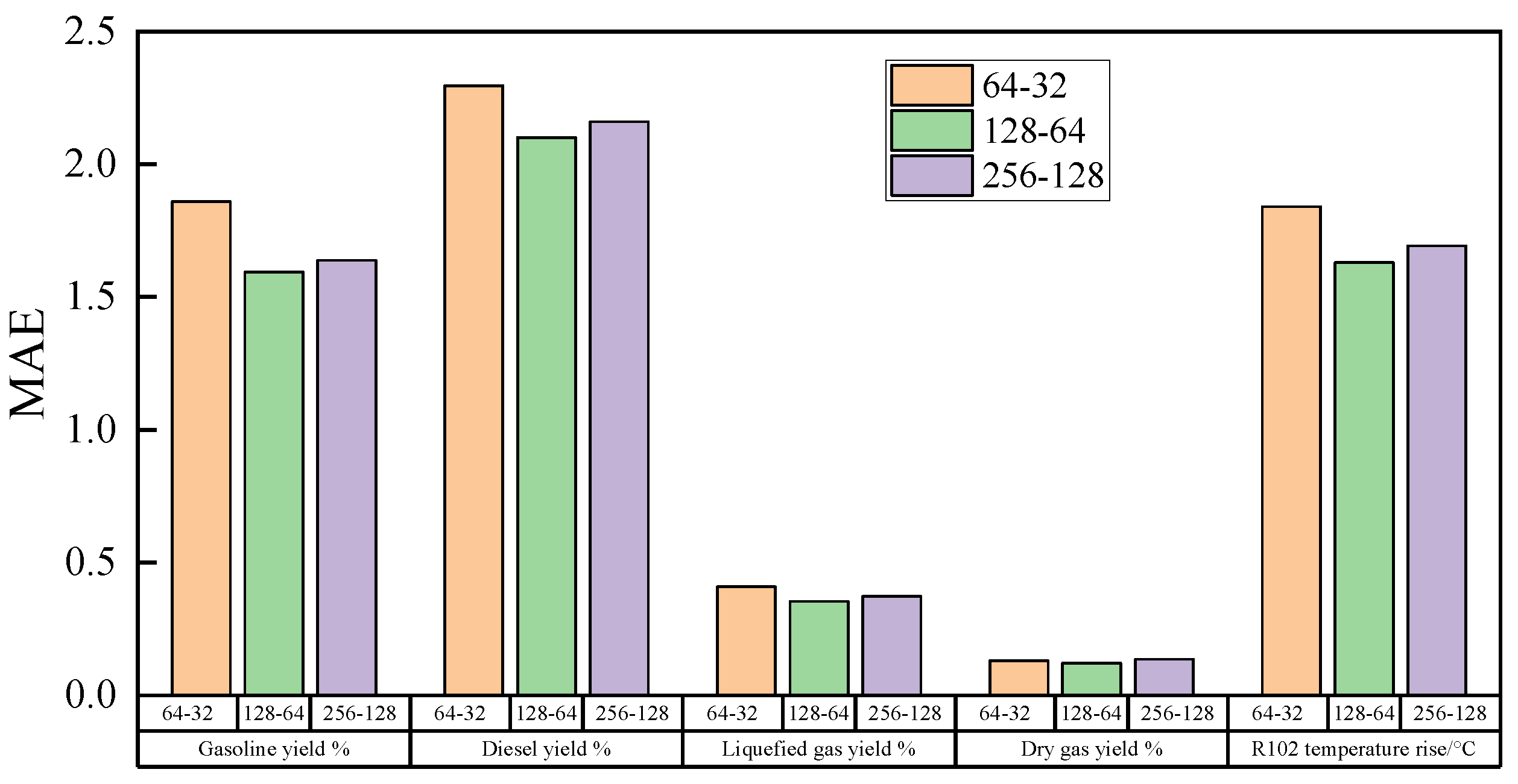
Determination of the number of neurons in the hidden layer

The greater the number of hidden layers and the number of neurons in the layer, the more complex the model and the easier it is to overfit [21,22]. Conversely, if the number of hidden layers and the number of neurons in the layer are too small, the learning ability of the model will be reduced and it will be easy to overfit. Therefore, setting the number of hidden layers and the number of neurons in the layer to match the complexity of the modeling data is essential to ensure the learning ability and generalization ability of the model.

As the amount of data in this paper is up to 974 groups, two hidden layers were chosen to enhance the learning ability of the model. For the number of neurons in the hidden layers, this study first determined three different combinations of the number of neurons in the hidden layers 64-32, 128-64, and 256-128 (the two numbers represent the number of neurons in the first and second hidden layers, respectively), with different combinations representing different models. The different combinations represent different model complexities, and then the optimal combination was determined by comparing the prediction results of the testing set under different combinations. Figure 3 shows the comparison of the prediction results of the model with different combinations of the number of hidden layer neurons. From Figure 3, it is evident that, for the five prediction targets of gasoline yield, diesel yield, LPG yield, dry gas yield, and R102 temperature rise, the combination of the number of hidden layer neurons (128-64) achieved the lowest MAE and the best prediction effect. Therefore, the number of neurons in the first and second hidden layers was determined to be 128 and 64, respectively.

(5)

Choice of activation function

The activation function in the DNN is mainly used to perform non-linear mapping, thus enhancing the fitting ability of the model [23]. Commonly used activation functions include Sigmoid, Tanh, ReLU, etc., which are calculated as in Equations (4) to (6), respectively [24]. The sigmoid function has continuous and bounded outputs, making it beneficial for network propagation as it prevents data from diverging. Additionally, the sigmoid function can perform self-regulation, which aids in updating network parameters during backpropagation. Furthermore, the Tanh function has outputs centered around zero, while the ReLU function is simple and efficient. However, the ReLU function may lead to some neurons not being activated due to its one-sided inhibition.

Different activation functions have varying adaptability for different tasks. Therefore, it is essential to compare the performance of each of the three activation functions (sigmoid, Tanh, and ReLU) in the prediction of the RLG device. This comparison will help to determine the optimal activation function for the task.

$$ReLU(x)=max(0,x)$$

(4)

$$tanh(x)=\frac{e^x-e^{-x}}{e^x+e^{-x}}$$

(5)

$$sigmoid(x)=\frac{1}{1+e^{-x}}$$

(6)

Figure 4 shows the curve of the loss of the testing set with the number of training sessions when the model uses different activation functions. The Tanh and ReLU functions converge faster than the sigmoid function at the initial stage, but the final errors are both higher than the sigmoid function, and the fluctuations during the training process are larger, which is not conducive to the smooth learning of the model. Therefore, the optimal activation function was determined to be the sigmoid function.

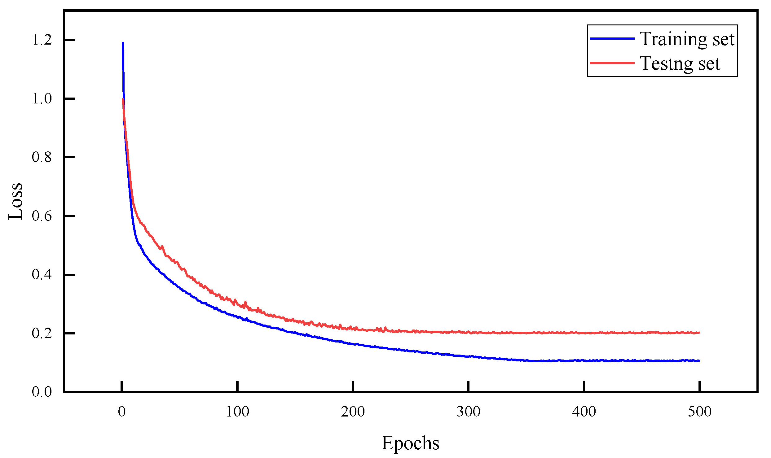
4.1.2. DNN Model Training

After determining the model parameters, the network structure is as depicted in Figure 5. The input layer consists of 17 input variables, such as fresh diesel feed. The 2 hidden layers have 128 and 64 neurons, respectively. The activation function used is sigmoid, and a BN layer is incorporated. The output layer comprises five variables, including gasoline yield.

The mean squared error (MSE) was used as the loss function for the DNN model to measure the deviation between the predicted values and the actual values. As shown in Equation (7), the loss function is the mean squared error of the four product yields and the temperature rise R102 of the RLG device. The model was trained using the Adam algorithm [25], and the loss curves for the training and testing sets during the training process are shown in Figure 6. After 350 iterations, the loss for both the training and testing sets remains relatively unchanged, indicating that the model has converged at this point and that further training will not improve the prediction accuracy of the model. The model achieves a low loss value for both the training and testing sets, indicating that training can be stopped and evaluation metrics can be used to assess the predictive performance of the model.

$$\begin{array}{l}loss(x)=\frac{1}{n}{\displaystyle \sum _{i=1}^n[}{\left(f_1(x)-y_1\right)}^2+{\left(f_2(x)-y_2\right)}^2+{\left(f_3(x)-y_3\right)}^2+\\ {\left(f_4(x)-y_4\right)}^2+{\left(f_5(x)-y_5\right)}^2]\end{array}$$

(7)

where $f_1(x)$~$f_5(x)$ are the predicted values of the DNN model for gasoline yield, diesel yield, LPG yield, dry gas yield, and R102 temperature rise, respectively; and y₁~y₅ represent the actual values of each, respectively.

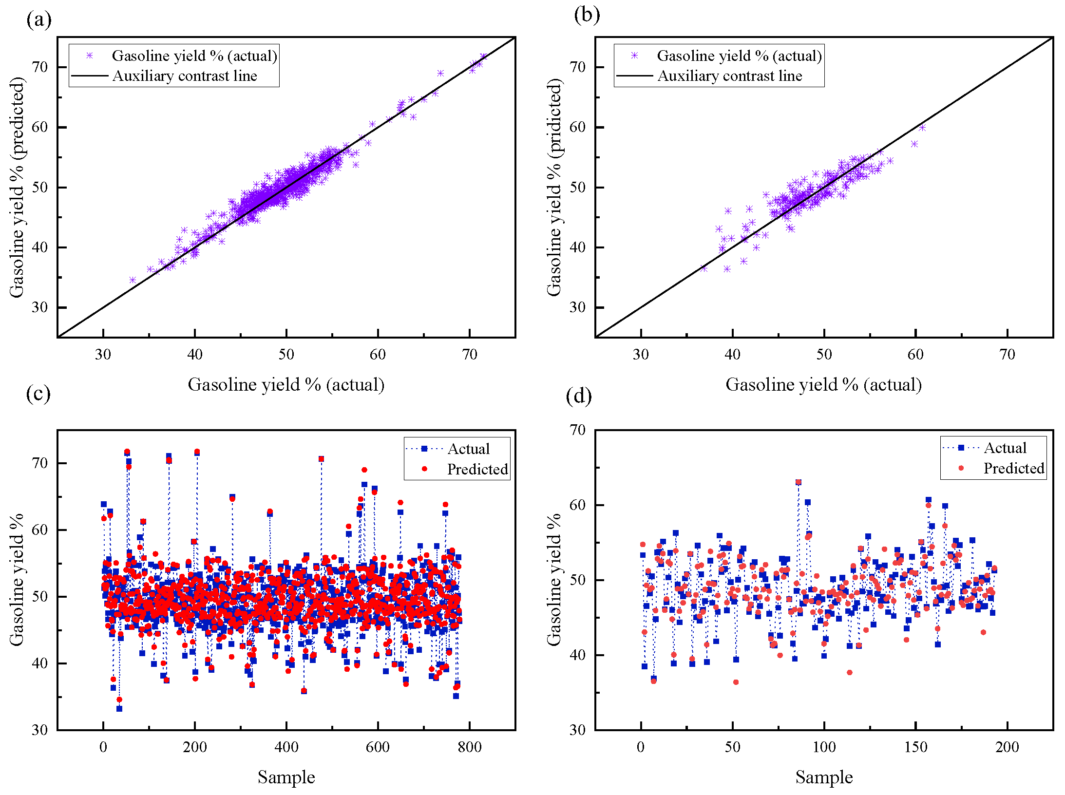
4.1.3. Model Prediction Results and Evaluation

Table 3. Evaluation indexes for training set of DNN model.

Program	Gasoline Yield	Diesel Yield	LPG Yield	Dry Gas Yield	R102 Temperature Rise
MAE	0.9122	1.0565	0.2382	0.0987	0.9671
MSE	1.4305	2.0185	0.1030	0.0171	1.7750
R2	0.9370	0.9333	0.9469	0.9266	0.9603
MAPE	0.0188	0.0262	0.1040	0.0467	0.0202

and

Table 4. Evaluation indexes for testing set of DNN model.

Program	Gasoline Yield	Diesel Yield	LPG Yield	Dry Gas Yield	R102 Temperature Rise
MAE	1.5810	1.9810	0.3519	0.1290	1.5575
MSE	6.8294	10.6909	0.4005	0.0283	7.7243
R2	0.7252	0.6929	0.7843	0.8811	0.7891
MAPE	0.0370	0.0469	31.2087	0.0615	0.0300

display the evaluation metrics of the DNN prediction model on 779 training samples and 195 testing samples, respectively. In the training set, the model performs well in predicting the production of the four main products in the RLG device. In the training set, the MAE for gasoline and diesel yield is approximately 1%, while the MAE for LPG yield is around 0.2%, and the MAE for dry gas yield is only 0.1%. This indicates that the model is able to learn hidden patterns in the factory data and make highly accurate predictions for each product’s yield. In the testing set, the model still achieves good prediction results, with a slightly higher MAE compared to the training set. The MAE for gasoline and diesel yield is below 2%, while the MAE for LPG and dry gas yield is below 0.4%. These results meet the requirements for estimating accuracy in practical industrial applications. The model not only demonstrates a good predictive performance on the training set but also exhibits a high prediction accuracy on the testing set, indicating its strong generalization ability for practical industrial predictions. In addition to the production of these four products, the model can also make more accurate predictions for the temperature rise of R102. The MAE for the temperature rise of R102 in the testing set is 1.5575 °C, which indicates a small deviation and provides important reference for temperature monitoring in practical industrial applications.

The scatter distribution of the actual and predicted gasoline yields and the comparison is shown in Figure 7. The accuracy and precision of the predictions for each product yield training and testing set can be visualized from the scatter plots.

Figure 7a,b show the deviation between the actual gasoline production values and the predicted gasoline production values in both the training set and the testing set. Figure 7b shows that the actual and predicted gasoline yield values in the testing set are still well concentrated around the diagonal line, indicating that the prediction performance of the testing set is still good. The good predictive results on the training set indicate that the model has successfully learned the underlying patterns in the data. Even though the testing set data were not part of the model’s training, the small deviation between the actual values and predicted values on the testing set demonstrates that the model performs well and has a good predictive accuracy and generalization ability on new samples.

Figure 7c,d show the comparison between the actual and predicted gasoline yield values on the training and testing sets, respectively. The model’s good performance on the testing set, where the actual and predicted values are close to each other, indicates that the model has a strong generalization ability and can make reliable predictions for new samples.

4.2. Mathematical Model for Revenue Optimization of RLG Device

Plant revenue consists of two levels of problems, namely the development of mathematical models and the use of optimization algorithms to solve them. A predictive model for the main indicators of the RLG device was developed. In accordance with the actual production requirements of the plant and the targets proposed in the direction of efficiency optimization, the optimization objective of this study was to maximize the output of the plant and, at the same time, increase the gasoline output by 3%.

4.2.1. The Objective Function of the Optimization Problem

Optimization problems can be categorized into two different types based on the form of the objective function: single-objective and multi-objective. In multi-objective optimization, the problem is decomposed into multiple single-objective functions, which are then combined as a weighted sum. The weights assigned to individual objective functions can be adjusted based on their relative importance, as shown in Equation (8).

$$F(x)={\alpha }_1\cdot f_1(x)+{\alpha }_2\cdot f_2(x)+\mathrm{\dots }+{\alpha }_k\cdot f_k(x)f_1(x),f_2(x),\mathrm{\dots },f_k(x)$$

(8)

where $F(x)$ is the weighted objective function; ${\alpha }_k$ is the weighting factor; $f_k(x)$ is a multiple objective function before weighting.

The objective of this paper was to maximize the return on the plant, which is the combined benefit of each product. The objective function of the optimization problem can be obtained by a weighted combination of the yield of each product and its unit price. As the price of oil products fluctuates with the market environment and is not a stable value, the unit price of each product in the objective function can be set dynamically with the market environment. In this paper, the current unit price of oil products in the refinery was used as a reference, where the unit price of gasoline is 7000 CNY/ton, the unit price of diesel is 5800 CNY/ton, the unit price of liquefied gas is 5848 CNY/ton, and the unit price of dry gas is 3000 CNY/ton; thus, the objective function is obtained as in Equation (9).

$$\max : F(X)=7000·f_1(X;W)+5800·f_2(X;W)+5848·f_3(X;W)+3000·f_4(X;W)$$

(9)

where X is an input variable to the predictive model for the main indicators of the RLG installation; $f_1(X;W)$ is a neural network prediction model for blended gasoline yields; $f_2(X;W)$ is a neural network prediction model for diesel yields; $f_3(X;W)$ is a neural network prediction model for liquefied gas yields; $f_4(X;W)$ is a neural network prediction model for dry gas yields; W is the neural network parameter.

4.2.2. Binding Conditions

The eight process parameters in the model, such as the average temperature of R101 and the partial pressure of inlet hydrogen selected here, were optimized by the optimization algorithm to maximize the objective function in Equation (8). Physical variables such as fresh diesel feed in the model input variables should remain unchanged during optimization at the time of optimization. The process parameters should be optimally adjusted based on the specific feed conditions (physical variables) to maximize the factory output.

In the optimization process, the search interval of the process parameters should meet the stability requirements of the device and the safe operating range, and the adjusted process parameters cannot make the temperature rise of the R102 reactor exceed 63 °C, otherwise it will bring safety hazards to the production of the device. Furthermore, in order to meet the company’s product distribution requirements, it is necessary to increase gasoline production by at least 3% while maximizing plant efficiency.

The above constraints form the constraints for optimizing the output of the RLG device, expressed in mathematical Equations (10) to (13), and are complicated by the presence of a series of non-linear constraints in the constraints.

$$s.t.x_1,x_2,x_3,x_4,x_5,x_6,x_7,x_8,x_9={\overline{x}}_1,{\overline{x}}_2,{\overline{x}}_3,{\overline{x}}_4,{\overline{x}}_5,{\overline{x}}_6,{\overline{x}}_7,{\overline{x}}_8,{\overline{x}}_9$$

(10)

$$l{b}_i\le x_i\le u{b}_{i } ; i=10,11,12,13,14,15,16,17$$

(11)

$$\mathrm{binding} \mathrm{conditions} f_1(X;W)-f_1(\overline{X};W)\ge 3\%$$

(12)

$$f_5(X;W)\le 63$$

(13)

where $\overline{x_1}$~$\overline{x_9}$ are the values of the nine physical variables before optimization, which remain constant during the optimization process; $x_{10}$~$x_{17}$ are the upper and lower limits of the eight process parameters to be optimized, and lb is the lower limit of the variable constraint; ub is the upper limit of the variable constraint; $f_1(X,W)$ is the neural network prediction model for gasoline yield, where the optimized gasoline yield needs to be increased by 3%; $f_5(X,W)$ is the neural network prediction model for the temperature rise of R102, optimized to not exceed 63 °C.

4.2.3. Genetic Algorithm to Optimize RLG Device Yield

(1)

Parameter setting of the genetic algorithm

For the mathematical model constructed for the optimization of the RLG device revenue, the GA can be used to optimize the search for process parameters and maximize the plant revenue while satisfying the constraints. The GA in this section is coded with real numbers and each individual is a string of real numbers [13,26,27]. The results of the device gain prediction in the process of calculating the extremes are used as individual fitness values and are calculated as follows:

$$F_i=y_{profit}$$

(14)

where F_i is the individual’s fitness value and y_profit is the predicted return on the installation for individual i.

The roulette wheel method was used to select individuals with a large proportion of adaptation into the next generation, calculated as follows:

$$f_i=k\ast F_i$$

(15)

$$p_i=\frac{f_i}{{\displaystyle \sum _{j=1}^N{f}_i}}$$

(16)

where F_i and f_i are the fitness value of the individual, p_i is percentage of adaptation, k is the coefficientand N is the population size,

(2)

RLG device yield optimization results

Based on a mathematical model for optimizing the profits of the RLG unit, a genetic algorithm can be used to search for the optimal process parameters based on different feed characteristics and the purity of recycled hydrogen gas in order to maximize the profits of the unit while satisfying the constraints. To study the applicability of the yield optimization model under different feed conditions, the yields of 974 samples were optimized, with 9 process parameters to be optimized for each sample, as shown in

Table 5. Process condition optimization space.

Process Conditions	Space for Excellence
R101 average temperature (°C)	360~395
R101 Inlet hydrogen partial pressure (MPa)	6.5~9.1
R101 inlet circulating hydrogen flow rate (kN3/h)	120~140
R101 inlet hydrogen-to-oil ratio	800~1200
R102 average temperature (°C)	370~415
R102 inlet hydrogen partial pressure (MPa)	6.5~9.1
R102 inlet circulating hydrogen flow rate (kN3/h)	130~150
R102 inlet hydrogen-to-oil ratio	900~1400

. To examine the applicability of the yield optimization model under different feed conditions, the plant yields for each sample out of the 974 were optimized, and the yields, gasoline production, and R102 temperature increase before and after optimization were compared.

Figure 8 shows the plant revenue before and after optimization for the 974 groups of samples. The plant revenue of the samples after optimization was higher than that before optimization, indicating the effectiveness of the revenue optimization model. The average plant yield before optimization was CNY 6000.70 per ton and, after optimization, the average plant yield was CNY 6290.75 per ton, an increase of CNY 290.05 per ton of product, which is a significant improvement in yield.

Figure 9 shows the gasoline yields before and after optimization for group 974 samples, all of which were improved to varying degrees after the model optimization. The average gasoline yield before optimization was 49.31% and the average gasoline yield after optimization was 52.96%, an average increase of 3.65% in gasoline yield, which is in line with the plant’s requirement for a 3% increase in gasoline yield in the product.

Figure 10 shows the temperature rise of R102 before and after the optimization of 974 samples. In practical production, when the temperature increase of R102 exceeds 63 °C, it poses a safety risk to the operation of the unit. Before optimization, there were a few samples with R102 temperature increases exceeding 63 °C. After optimization, the temperature increase of R102 is below 63 °C, ensuring the stable operation of the plant.

A total of 4 groups of samples were randomly selected from the 974 groups and their process parameters before and after optimization are shown in

Table 6. GA optimizing process conditions results.

Process Conditions	Group 1		Group 2		Group 3		Group 4
	Original Value	Optimization Value	Original Value	Optimization Value	Original Value	Optimization Value	Original Value	Optimization Value
R101 average temperature (°C)	370.3	377.2	381.3	390.5	367.2	376.7	371.2	378.5
R101 inlet hydrogen partial pressure (MPa)	6.9	6.8	8.5	9.10	6.7	6.7	7.9	7.1
R101 inlet circulating hydrogen flow rate (kN3/h)	148	132	132	140	153	124	153	140
R101 inlet hydrogen-to-oil ratio	1435	1200	1232	800	1518	1200	11,451	1200
R102 average temperature (°C)	375.8	377.7	381.9	391.0	381.8	383.4	388.6	398.5
R102 inlet hydrogen partial pressure (MPa)	6.85	6.80	8.48	9.01	6.63	6.58	7.78	6.94
R102 inlet circulating hydrogen flow rate (kN3/h)	155	146	145	145	160	145	160	142
R102 inlet hydrogen-to-oil ratio	1506	1400	1357	900	1591	1400	1516	1400
R102 temperature rise (°C)	58.8	60.4	59.96	60.5	57.9	60.0	61.0	63.0
Gasoline yield%	53.86	57.01	52.10	55.31	49.10	52.11	49.71	53.62
Plant revenue (CNY/ton)	6240	6382	6030	6381	6269	6331	6083	6302

. It can be seen that the increase in plant yield is in the same direction as the increase in gasoline yield. When the average temperature of R101 and R102 is increased, the gasoline yield is increased by more than 3% and the plant economy is improved; however, the actual increase in temperature of the two reactors cannot exceed 10 °C. If the temperature is increased too high, even though the theoretical gasoline yield will be improved, the subsequent sacrifice is the catalyst life and the destruction of the plant. The industrial reference significance is lost as the product distribution structure is destroyed. At the same time, the temperature rise limit for R102 must not exceed 63 °C. The optimization model does not exceed the temperature of R102, which means that the temperature optimization is reasonable. The actual factor of the reaction pressure is the hydrogen partial pressure. In general, the hydrogen partial pressure increases and the gasoline yield increases, but the premise needs to be that the hydrogen partial pressure can be increased slowly to increase the gasoline yield if the gasoline RON meets the requirements [28]; at the same time, the hydrogen partial pressure increases as the circulating hydrogen flow rate and hydrogen–oil ratio increase. The hydrogen-to-oil ratio is controlled and regulated by the circulating hydrogen flow rate. An increase in the hydrogen-to-oil ratio reduces the residence time of the reactants in the catalyst bed, which is not conducive to the hydrogenation reaction [29]. Referring to Table 6, it can be seen that the optimization space for the hydrogen–oil ratio and the inlet circulating hydrogen flow rate for both reactors is adjusted downwards compared to the actual operating conditions, which corresponds to a slight decrease in the optimized hydrogen partial pressure, indicating that the optimization direction is in line with the industrial operation. Therefore, the results of this paper using genetic algorithms to optimize the process conditions are consistent with the actual hydrocracking process principles, and the results are of some significance for industrial operation.

5. Conclusions

Through collecting and mining the raw material and product composition analysis data of the RLG device, this study used a DNN to establish a prediction and optimization model for product distribution.

• First, by combining the reaction mechanism and characteristics of the RLG process, data such as the properties of the crude oil and process operation variables were separated and preprocessed. A three-layer DNN model with (17, 128, 64) nodes was then established. This model predicts the gasoline yield with an average absolute error of 1.58%, showing a better prediction performance.
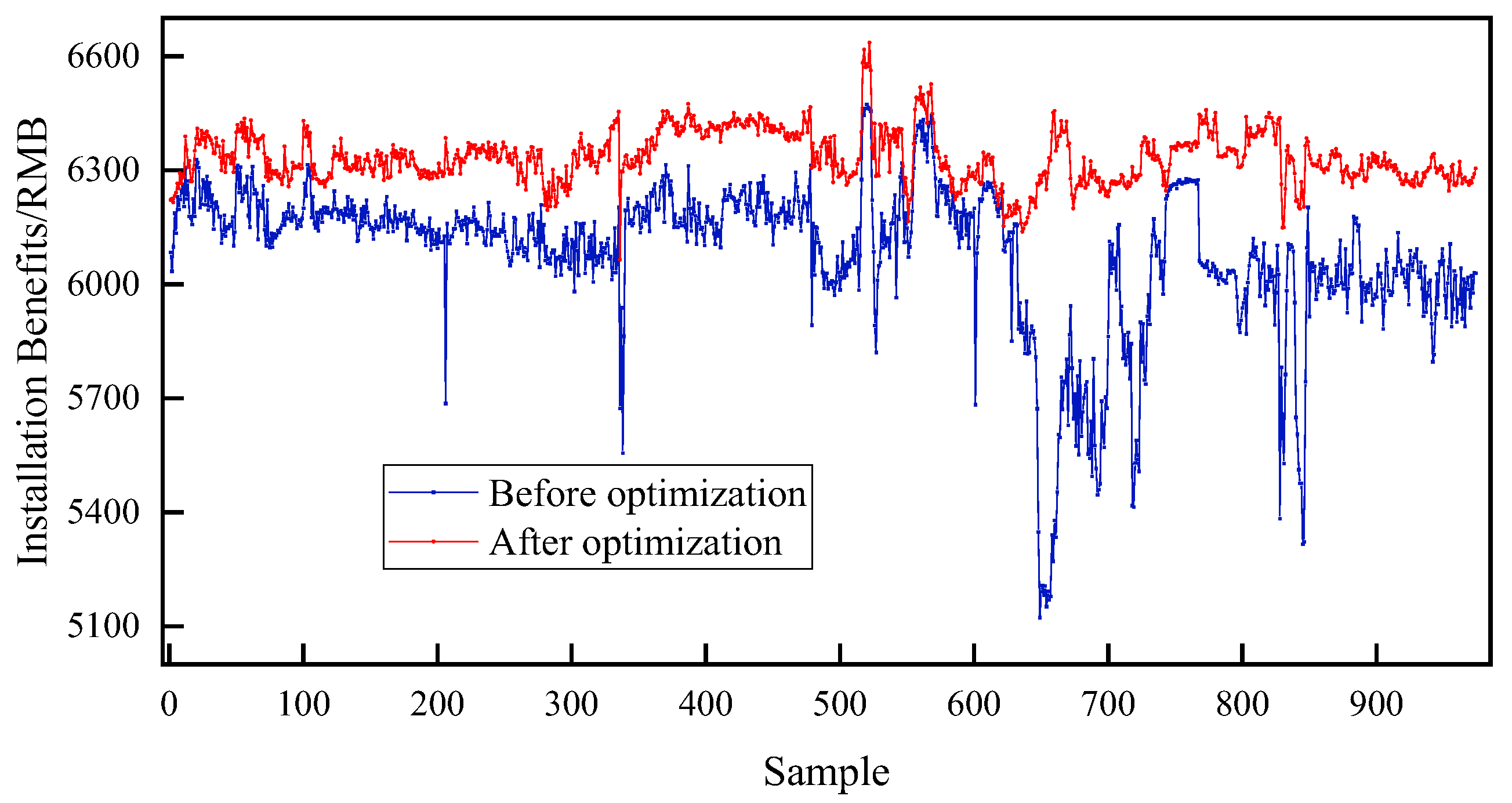
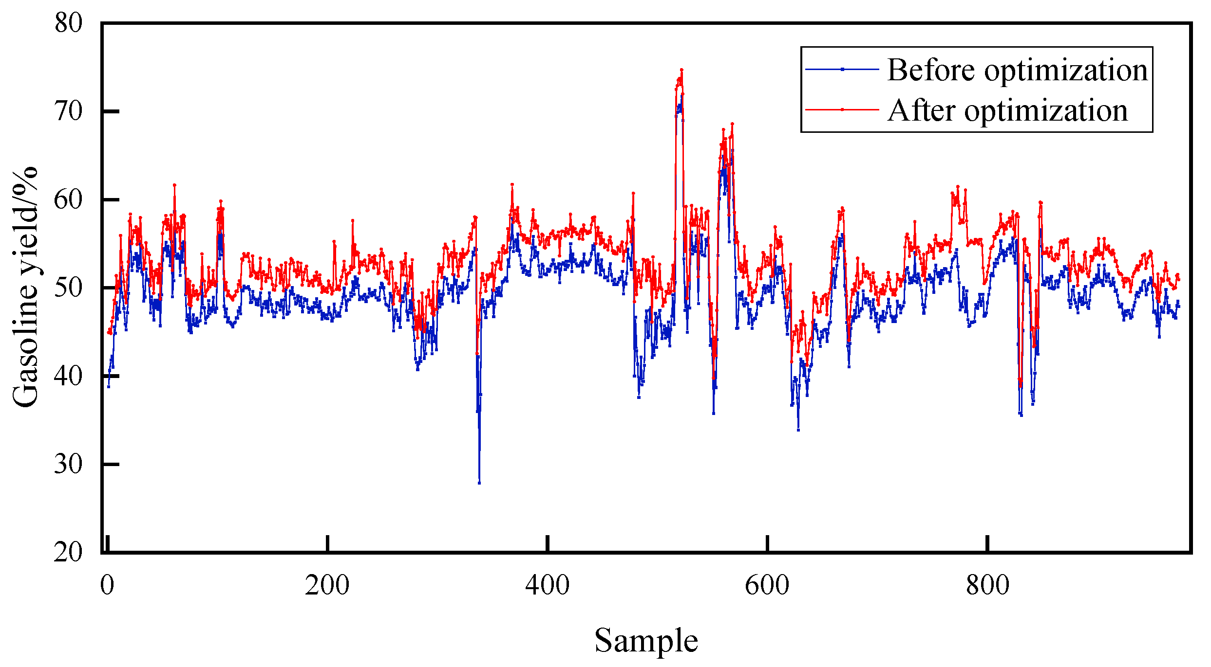
• Then, on the basis of this predictive model, plant tuning operations were carried out with the goal of maximizing plant efficiency.
• Next, the results show that optimizing the operating conditions using the GA algorithm to meet the 3% increase in gasoline production can maximize the economic benefits of the plant.
• Finally, it was verified that the optimization value of the operating conditions is consistent with the actual situation of the RLG process, which proves that the established model has good applicability.

References

1. Song, W.; Du, W.; Fan, C.; Yang, M.; Qian, F. Adaptive Weighted Hybrid Modeling of Hydrocracking Process and Its Operational Optimization. Ind. Eng. Chem. Res. 2021, 60, 3617–3632. [Google Scholar] [CrossRef]
2. Stangeland, B.E. A kinetic model for the prediction of hydrocracker yields. Ind. Eng. Chem. Process Des. Dev. 1974, 13, 71–76. [Google Scholar] [CrossRef]
3. Laxminarasimhan, C.S.; Verma, R.P.; Ramachandran, P.A. Continuous lumping model for simulation of hydrocracking. AIChE J. 1996, 42, 2645–2653. [Google Scholar] [CrossRef]
4. Mohanty, S.; Saraf, D.N.; Kunzru, D. Modeling of a hydrocracking reactor. Fuel Process. Technol. 1991, 29, 1–17. [Google Scholar] [CrossRef]
5. Pacheco, M.A.; Dassori, C.G. Hydrocracking: An improved kinetic model and reactor modeling. Chem. Eng. Commun. 2002, 189, 1684–1704. [Google Scholar] [CrossRef]
6. Thybaut, J.W.; Marin, G.B. Multiscale aspects in hydrocracking: From reaction mechanism over catalysts to kinetics and industrial application. In Advances in Catalysis; Academic Press: Cambridge, MA, USA, 2016; Volume 59, pp. 109–238. [Google Scholar]
7. Song, W.; Mahalec, V.; Long, J.; Yang, M.-L.; Qian, F. Modeling the Hydrocracking Process with Deep Neural Networks. Ind. Eng. Chem. Res. 2020, 59, 3077–3090. [Google Scholar] [CrossRef]
8. Chen, Q.; Ding, J.; Yang, S.; Chai, T. Constrained Operational Optimization of a Distillation Unit in Refineries With Varying Feedstock Properties. IEEE Trans. Control. Syst. Technol. 2019, 28, 2752–2761. [Google Scholar] [CrossRef]
9. Taud, H.; Mas, J.F. Multilayer perceptron (MLP). In Geomatic Approaches for Modeling Land Change Scenarios; Springer: Cham, Switzerland, 2018; pp. 451–455. [Google Scholar]
10. Hussain, H.; Tamizharasan, P.S.; Rahul, C.S. Design possibilities and challenges of DNN models: A review on the perspective of end devices. Artif. Intell. Rev. 2022, 55, 5109–5167. [Google Scholar] [CrossRef]
11. Belghazi, M.I.; Baratin, A.; Rajeshwar, S.; Ozair, S.; Bengio, Y.; Courville, A.; Hjelm, D. Mutual information neural estimation. In Proceedings of the International Conference on Machine Learning, PMLR, Stockholm, Sweden, 10–15 July 2018; pp. 531–540. [Google Scholar]
12. Hu, L.; Gao, L.; Li, Y.; Zhang, P.; Gao, W. Feature-specific mutual information variation for multi-label feature selection. Inf. Sci. 2022, 593, 449–471. [Google Scholar] [CrossRef]
13. Ileberi, E.; Sun, Y.; Wang, Z. A machine learning based credit card fraud detection using the GA algorithm for feature selection. J. Big Data 2022, 9, 1–17. [Google Scholar] [CrossRef]
14. Lira, J.O.; Riella, H.G.; Padoin, N.; Soares, C. Computational fluid dynamics (CFD), artificial neural network (ANN) and genetic algorithm (GA) as a hybrid method for the analysis and optimization of micro-photocatalytic reactors: NOx abatement as a case study. Chem. Eng. J. 2021, 431, 133771. [Google Scholar] [CrossRef]
15. Huang, C.L.; Dun, J.F. A distributed PSO–SVM hybrid system with feature selection and parameter optimization. Appl. Soft Comput. 2008, 8, 1381–1391. [Google Scholar] [CrossRef]
16. Ghannadi, P.; Kourehli, S.S.; Mirjalili, S. A review of the application of the simulated annealing algorithm in structural health monitoring (1995–2021). Frat. Ed Integrità Strutt. 2023, 17, 51–76. [Google Scholar] [CrossRef]
17. Dubey, A.K.; Kumar, A.; Agrawal, R. An efficient ACO-PSO-based framework for data classification and preprocessing in big data. Evol. Intell. 2021, 14, 909–922. [Google Scholar] [CrossRef]
18. Citovsky, G.; DeSalvo, G.; Gentile, C.; Karydas, L.; Rajagopalan, A.; Rostamizadeh, A.; Kumar, S. Batch active learning at scale. Adv. Neural Inf. Process. Syst. 2021, 34, 11933–11944. [Google Scholar]
19. Lobacheva, E.; Kodryan, M.; Chirkova, N.; Malinin, A.; Vetrov, D.P. On the periodic behavior of neural network training with batch normalization and weight decay. Adv. Neural Inf. Process. Syst. 2021, 34, 21545–21556. [Google Scholar]
20. Santurkar, S.; Tsipras, D.; Ilyas, A.; Madry, A. How does batch normalization help optimization? In Proceedings of the Advances in Neural Information Processing Systems, Montreal, QC, Canada, 3–8 December 2018; Volume 31. [Google Scholar]
21. Zhao, Q.; Chen, X.; Zhang, Y.; Sha, M.; Yang, Z.; Lin, W.; Tang, E.; Chen, Q.; Li, X. Synthesizing ReLU neural networks with two hidden layers as barrier certificates for hybrid systems. In Proceedings of the 24th International Conference on Hybrid Systems: Computation and Control, Nashville, TN, USA, 19–21 May 2021; pp. 1–11. [Google Scholar]
22. Sun, J.; Wang, J.; Zhu, Z.; He, R.; Peng, C.; Zhang, C.; Huang, J.; Wang, Y.; Wang, X. Mechanical Performance Prediction for Sustainable High-Strength Concrete Using Bio-Inspired Neural Network. Buildings 2022, 12, 65. [Google Scholar] [CrossRef]
23. Hong, Q.; Tan, Q.; Siegel, J.W.; Xu, J. On the activation function dependence of the spectral bias of neural networks. arXiv 2022, arXiv:2208.04924. [Google Scholar]
24. Tian, Y.; Lai, Y.; Yang, C. Research of consumption behavior prediction based on improved DNN. Sci. Program. 2022, 2022, 6819525. [Google Scholar] [CrossRef]
25. Reyad, M.; Sarhan, A.M.; Arafa, M. A modified Adam algorithm for deep neural network optimization. Neural Comput. Appl. 2023, 1–18. [Google Scholar] [CrossRef]
26. Saini, M.; Gupta, N.; Shankar, V.G.; Kumar, A. Stochastic modeling and availability optimization of condenser used in steam turbine power plants using GA and PSO. Qual. Reliab. Eng. Int. 2022, 38, 2670–2690. [Google Scholar] [CrossRef]
27. Abdi, H. Profit-based unit commitment problem: A review of models, methods, challenges, and future directions. Renew. Sustain. Energy Rev. 2020, 138, 110504. [Google Scholar] [CrossRef]
28. Martínez, J.; Zúñiga-Hinojosa, M.A.; Ruiz-Martínez, R.S. A Thermodynamic Analysis of Naphtha Catalytic Reforming Reactions to Produce High-Octane Gasoline. Processes 2022, 10, 313. [Google Scholar] [CrossRef]
29. Lahijani, P.; Mohammadi, M.; Mohamed, A.R.; Ismail, F.; Lee, K.T.; Amini, G. Upgrading biomass-derived pyrolysis bio-oil to bio-jet fuel through catalytic cracking and hydrodeoxygenation: A review of recent progress. Energy Convers. Manag. 2022, 268, 115956. [Google Scholar] [CrossRef]
Figure 1. Schematic diagram of a typical RLG device flow.
Energies 16 05332 g001
Figure 2. Reciprocal information between model input variables and gasoline yields.
Energies 16 05332 g002
Figure 3. MAE of each output on the testing set for different combinations of the number of hidden layer neurons.
Energies 16 05332 g003
Figure 4. Loss curve on the testing set with different activation functions.
Energies 16 05332 g004
Figure 5. The network structure of the DNN prediction model for RLG device.
Energies 16 05332 g005
Figure 6. Loss graph.
Energies 16 05332 g006
Figure 7. Comparison of the difference between actual and predicted gasoline yields. (a) Dispersion between actual and predicted petrol yields on the training sets; (b) Dispersion between actual and predicted gasoline yields on the testing sets; (c) Distribution of actual gasoline yield and predicted gasoline yield values on the training sets; (d) Distribution of actual gasoline yield and predicted gasoline yield values on the testing sets.
Energies 16 05332 g007
Figure 8. Comparison chart before and after optimization for plant revenue.
Energies 16 05332 g008
Figure 9. Comparison chart before and after optimization for gasoline yield.
Energies 16 05332 g009
Figure 10. Comparison chart before and after optimization for R102 temperature rise.
Energies 16 05332 g010