Generalized Regression Neural Network Based Meta-Heuristic Algorithms for Parameter Identification of Proton Exchange Membrane Fuel Cell

Abstract

An accurate parameter extraction of the proton exchange membrane fuel cell (PEMFC) is crucial for establishing a reliable cell model, which is also of great significance for subsequent research on the PEMFC. However, because the parameter identification of the PEMFC is a nonlinear optimization problem with multiple variables, peaks, and a strong coupling, it is difficult to solve this problem using traditional numerical methods. Furthermore, because of insufficient current and voltage data measured by the PEMFC, the precision rate of cell parameter extraction is also very low. The study proposes a parameter extraction method using a generalized regression neural network (GRNN) and meta-heuristic algorithms (MhAs). First of all, a GRNN is used to de-noise and predict the data to solve the problems in the field of PEMFC, which include insufficient data and excessive noise data of the measured data. After that, six typical algorithms are used to extract the parameters of the PEMFC under three operating conditions, namely high temperature and low pressure (HTLP), medium temperature and medium pressure (MTMP), and low temperature and high pressure (LTHP). The last results demonstrate that the application of GRNN can prominently decrease the influence of data noise on parameter identification, and after data prediction, it can greatly enhance the precision rate and reliability of MhAs parameter identification, specifically, under HTLP conditions, the V-I fitting accuracy achieved 99.39%, the fitting accuracy was 99.07% on MTMP, and the fitting accuracy was 98.70%.

1. Introduction

With the rapid development of technology and continuous economic growth, the demand for various fossil fuels and electricity is increasing day by day. The existing problem is that the energy conversion efficiency of traditional fossil energy is relatively low, and it causes huge environmental pollution, bringing the greenhouse effect, rising sea levels, acid rain, and other thorny environmental problems [1,2]. In addition, the massive development and utilization of traditional non-renewable energy will also cause the global energy crisis [3]. In this context, countries around the world have begun to vigorously develop clean energy and renewable energy. The proton exchange membrane fuel cell (PEMFC) is widely used because of the advantages of high energy density, high power generation efficiency, starting at a low temperature and a long working life [4,5].

With the widespread application of the PEMFC, precise modeling of batteries is crucial for optimizing the control of cell systems and improving cell power generation efficiency. Currently, there are many models for the PEMFC, including three-dimensional steady-state models [6] and electrochemical steady-state models [7]. Among them, electrochemical stability models can predict the state of batteries very well, it is beneficial for the safe and stable operation of the PEMFC and cell management. Accurate cell models rely on accurate internal model parameters, so accurate parameter identification of PEMFC batteries is a prerequisite for establishing accurate and reliable cell models. However, because the PEMFC parameter identification is a nonlinear problem with multiple variables, multiple peaks, a strong coupling, and limited V-I data measured by the cell, it is arduous to use traditional numerical analysis methods for parameter identification, for example, the least squares method, gradient descent method, and the identification results are not ideal [8]. However, meta-heuristic algorithms (MhAs) are widely used in the field of PEMFC parameter extraction due to their low initial value requirements and global search ability, which can avoid falling into local optimum [9].

A study [10] proposed an identification method based on adaptive focusing particle swarm optimization (AFPSO). Compared with particle swarm optimization (PSO), AFPSO has a stronger global search capability and faster optimization speed. Final experimental results also demonstrate that the obtained results have high fitting accuracy with the data obtained from experimental testing, and can effectively identify the parameters of the cell. In work [11], a PEMFC parameter estimation study based on an extended Kalman filter (EKF) was proposed. By constructing a semi-mechanistic and semi-empirical PEMFC model, based on the characteristics of the existing sensor signals in the model system, the EKF was used to extract parameters of the cell model. Specifically, this method estimates the parameters during PEMFC off-design operation, and it is more in line with the actual application of batteries. Work [12] uses an extreme learning machine (ELM) to identify cell parameters, where under the actual operating conditions, the measured current and voltage data will inevitably have exception values, that is, noise data, which will affect the identification accuracy of parameters in the model. Therefore, in this study, it is proposed to use ELM to train the data, then perform noise reduction processing, then use algorithms for parameter identification. The results obtained also prove that the data after noise reduction processing is used for parameter extraction, and the identification accuracy is significantly improved. In the literature [13], a PEMFC parameter identification study of improved chicken swarm optimization (ICSO) was proposed. In this paper, the author introduced a Tent mapping strategy to initialize the population, which can improve the uniformity and ergodicity of the population. Secondly, set adaptive inertia weights on the feeding speed of individual chickens, which can improve the optimization efficiency of individual hens, and the Levy flight strategy were introduced to randomly update the chicken position, greatly improving the algorithm’s global search ability. Finally, by comparing the parameter identification results obtained by ICSO with those obtained by other heuristic algorithms, it was proven that the ICSO algorithm has better parameter identification accuracy and a stronger model generalization ability. Reference [14] proposed an improved method based on a differential evolution algorithm, which is unique in that it references a probability selection model, which assigns a selection probability for every individual in the evolutionary population regarding their performance. In the work, to verify the effectiveness of algorithm, standard test functions were also used for testing. The experimental results showed that after the algorithm improvement, high data fitting accuracy can be achieved, and the parameters of the cell can be identified very accurately. In literature [15], a novel method based on the Levenberg Marquardt backpropagation (LMBP) algorithm was proposed. The neural network was designed based on the PEMFC model, and the LMBP algorithm was used for parameter identification. The LMBP is a variant of the Newton method, which combines the steepest descent method with the Gaussian Newton method and iteratively calculates using the Jacobian matrix, greatly improving computational efficiency. The final experimental results in the study also indicate that neural networks have higher fitting accuracy compared to heuristic algorithms, and the speed of parameter identification research through LMBP is much faster than that of heuristic algorithms. SOA is a swarm intelligence optimization algorithm that simulates the random search behavior of human beings. The SOA algorithm optimizes the parameters of the PEMFC model, and then compares the results with those of other algorithms, proving that the algorithm has good fitting accuracy, and it can significantly improve and enhance the accuracy of the PEMFC model parameters [16]. In reference [17], a PEMFC parameter identification method based on Bayesian regularization neural network (BRNN) was proposed. BRNN is used to de-noise data and MhAs are used to identify parameters, and the results are compared with other heuristic algorithms. The extraction results of BRNN data de-noising are more accurate than the original data results, and the results obtained are more stable with fewer outliers.

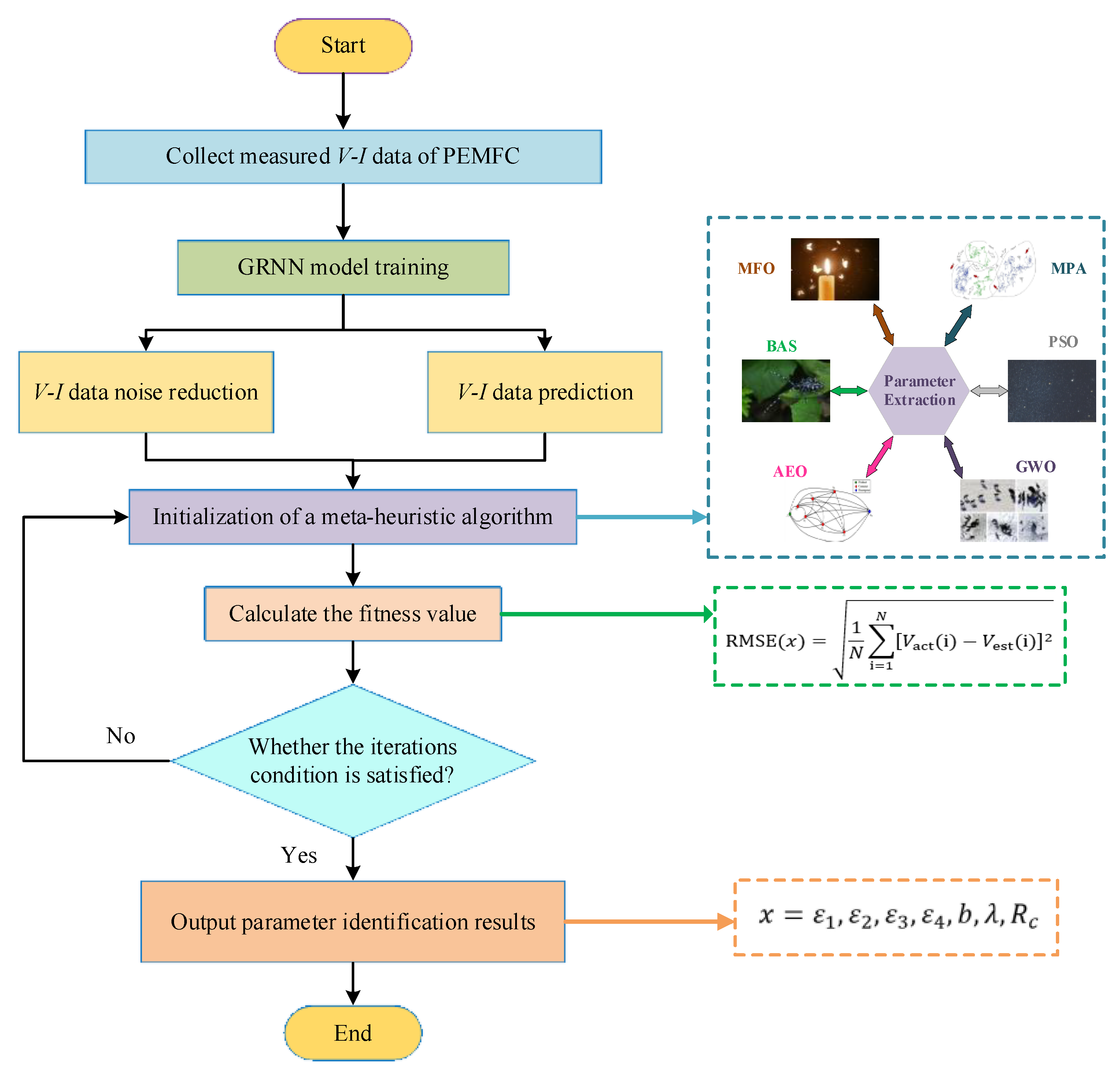
Overall, current research on PEMFC parameter identification mainly utilizes the MhAs method [18,19,20], and most of the research focuses on algorithm improvement to improve the accuracy and speed of parameter extraction. Only a few studies consider the impact of the data itself on the identification results. However, the study proposes MhAs based on a generalized regression neural network (GRNN) for PEMFC parameter extraction, which trains the GRNN, predicting and de-noising the data, fully considering the insufficient measured data and the impact of noise data on the final identification results, and conducting parameter identification research on the PEMFC under three operating conditions, namely high temperature and low pressure (HTLP), medium temperature and medium pressure (MTMP), and low temperature and high pressure (LTHP) [17]. The last results demonstrate that after data processing, its identification accuracy is higher and its performance is better. This study provides a new approach to the identification of PEMFC parameters, and its contributions and innovations can be summarized as follows:

• Established the PEMFC model and conducted parameter identification research on the model under three operating conditions;
• Considering the influence of insufficient data volume and noise data, a GRNN was used to de-noise and predict the measured V-I data, and the final results fully demonstrate its excellent robustness when applied to PEMFC parameter extraction under various operation conditions;
• Based on the data processed by a GRNN, six typical heuristic algorithms were compared for their effectiveness in PEMFC parameter identification. The results demonstrate that after data processing, accuracy can be greatly improved.

The structure of the remaining part is as follows: Section 2 is the modeling of the PEMFC, mainly introducing the internal chemical mechanism of PEMFC power generation and its cell model, and then establishing an objective function for the model. Section 3 mainly displays the application of GRNN-MhAs in PEMFC parameter identification research, which involves using a GRNN for data de-noising and prediction processing, and then using MhAs for parameter identification. Section 4 mainly displays the parameter identification results obtained by six algorithms under three working conditions. Section 5 is the discussion section. Section 6 provides some important conclusions obtained from this research, as well as some prospects for future PEMFC parameter identification research.

2. PEMFC Modeling

Establishing the PEMFC model is beneficial to conduct in-depth research on the parameter identification of a cell. This section mainly introduces the basic principles and mathematical models of the mechanism of the PEMFC.

2.1. The Mechanism of the PEMFC

In principle, the PEMFC is equivalent to a reverse device for water electrolysis. A typical PEMFC is composed of an anode, a cathode, and a proton exchange membrane. The anode is the site of hydrogen fuel oxidation, the cathode is the site of oxidant reduction, and both poles contain catalysts to accelerate electrode electrochemical reactions [21,22,23].

In addition, the electrochemical reaction mechanism of the PEMFC is shown in Equations (1)–(3) [24].

Anode side:

$${\mathrm{H}}_2\to 2{\mathrm{H}}^{+}+2{\mathrm{e}}^{-}$$

(1)

Cathode side:

$$\frac{1}{2}{\mathrm{O}}_2+2{\mathrm{H}}^{+}+2{\mathrm{e}}^{-}\to {\mathrm{H}}_2\mathrm{O}$$

(2)

Overall chemical reaction,

$${\mathrm{H}}_2+\frac{1}{2}{\mathrm{O}}_2\to {\mathrm{H}}_2\mathrm{O}$$

(3)

2.2. Mathematical Model of the PEMFC

The model introduced in this section is only one kind of cell model, namely the 0-D model. Note that many other multi-dimensional models exist. Considering the impact of some losses in electrochemical reactions on the output characteristics of the PEMFC, the output voltage is as follows [25]:

$$V_{\mathrm{est}}=E_{\mathrm{nernst}}-V_{\mathrm{act}}-V_{\mathrm{ohm}}-V_{\mathrm{con}}$$

(4)

where $V_{\mathrm{act}}$, $V_{\mathrm{ohm}}$ and $V_{\mathrm{con}}$, respectively, represent activation voltage loss (V), ohmic voltage loss (V), and concentration voltage loss (V); $E_{\mathrm{nernst}}$ is the thermodynamic electromotive force (V); $E_{\mathrm{nernst}}$ can be expressed as [26]:

$$E_{\mathrm{nernst}}=\frac{\Delta G}{2F}+\frac{\Delta S}{2F}\left(T_{\mathrm{k}}-T_{\mathrm{ref}}\right)+\frac{RT}{2F}\left[\ln \left(P_{{\mathrm{H}}_2}\right)+\frac{1}{2}\left(P_{{\mathrm{O}}_2}\right)\right]$$

(5)

where $\Delta G$ and $\Delta S$ represent changes in free Gibbs energy and entropy, respectively, the value of $\Delta G$ is 228,170 J/mol; $F$ represents a constant (96,485.3383 C/mol); $R$ is the universal gas constant (8.314 J/(K·mol)); $T_{\mathrm{k}}$ and $T_{\mathrm{ref}}$, respectively, represent the actual temperature and reference temperature; $T_{\mathrm{k}}$ has a value of 353.15 K under HTLP operating conditions, 333.15 K under MTMP operating conditions, and 313.15 K under operating conditions; $P_{{\mathrm{H}}_2}$ and $P_{{\mathrm{O}}_2}$ denote the partial pressure of hydrogen (atm) and oxygen (atm), which can be expressed as [27]:

$$P_{{\mathrm{H}}_2}=0.5\times R{H}_{\mathrm{a}}\times P_{{\mathrm{H}}_2\mathrm{O}}^{\mathrm{sat}}\times \left[{\left(\frac{R{H}_{\mathrm{a}}\times P_{{\mathrm{H}}_2\mathrm{O}}^{\mathrm{sat}}}{P_{\mathrm{a}}}\times \exp (\frac{1.635\left(\frac{i_{\mathrm{cell}}}{A}\right)}{T_{\mathrm{k}}^{1.334}})\right)}^{-1}-1\right]$$

(6)

$$P_{{\mathrm{O}}_2}=R{H}_{\mathrm{c}}\times P_{{\mathrm{H}}_2\mathrm{O}}^{\mathrm{sat}}\times \left[{\left(\frac{R{H}_{\mathrm{a}}\times P_{{\mathrm{H}}_2\mathrm{O}}^{\mathrm{sat}}}{P_{\mathrm{c}}}\times \exp (\frac{4.192\left(\frac{i_{\mathrm{cell}}}{A}\right)}{T_{\mathrm{k}}^{1.334}})\right)}^{-1}-1\right]$$

(7)

where $R{H}_{\mathrm{a}}$ and $R{H}_{\mathrm{c}}$ are the relative humidity of the vapor, the values of $R{H}_{\mathrm{a}}$ and $R{H}_{\mathrm{c}}$ are both 1 under HTLP operating conditions, 2 under MTMP operating conditions, and 3 under operating conditions; $P_{\mathrm{a}}$ and $P_{\mathrm{c}}$ the inlet pressure of the anode and cathode (atm), respectively; $i_{\mathrm{cell}}$ is the output current (A); $A$ is the effective activation area, the value of $\Delta G$ is 50.6 cm²; $P_{{\mathrm{H}}_2\mathrm{O}}^{\mathrm{sat}}$ is the saturation pressure (atm), which is as follows:

$${\log }_{10}\left(P_{{\mathrm{H}}_2\mathrm{O}}^{\mathrm{sat}}\right)=2.95\times {10}^{-2}\times T_{\mathrm{c}}-9.19\times {10}^{-5}\times T_{\mathrm{c}}^2+1.44\times {10}^{-7}\times T_{\mathrm{c}}^3-2.18$$

(8)

$$T_{\mathrm{c}}=T_{\mathrm{k}}-273.15$$

(9)

In addition, the activation voltage loss $V_{\mathrm{act}}$ can be expressed as:

$$V_{\mathrm{act}}={\epsilon }_1+{\epsilon }_2{T}_{\mathrm{k}}+{\epsilon }_3{T}_{\mathrm{k}}\ln \left(C_{{\mathrm{O}}_2}\right)+{\epsilon }_4{T}_{\mathrm{k}}\ln \left(i_{\mathrm{cell}}\right)$$

(10)

where ${\epsilon }_1$, ${\epsilon }_2$, ${\epsilon }_3$, and ${\epsilon }_4$ are semi-empirical coefficients; $C_{{\mathrm{O}}_2}$ denote the concentration of oxygen catalyzed by the anode catalyst surface (mol/cm³), which is shown below:

$$C_{{\mathrm{O}}_2}=\frac{P_{{\mathrm{O}}_2}}{5.08\times {10}^6\times {\mathrm{e}}^{\left(\frac{-498}{T_{\mathrm{k}}}\right)}}$$

(11)

In addition, the ohmic voltage $V_{\mathrm{ohm}}$ loss is as follows [28]:

$$V_{\mathrm{ohm}}=i_{\mathrm{cell}}\left(R_{\mathrm{m}}+R_{\mathrm{c}}\right)$$

(12)

where $R_{\mathrm{m}}$ and $R_{\mathrm{c}}$ are the electron transfer resistance and proton exchange membrane equivalent resistance (Ω), $R_{\mathrm{m}}$ can be expressed as:

$$R_{\mathrm{m}}={\rho }_{\mathrm{m}}\left(\frac{l}{A}\right)$$

(13)

where $l$ is the thickness of the proton exchange membrane, the value of $l$ is 178 $\mathsf{\mu }\mathrm{m}$; ${\rho }_{\mathrm{m}}$ represents the resistivity (Ω·cm), which can be expressed as:

$${\rho }_{\mathrm{m}}=\frac{181.6\times \left[1+0.03\times \left(\frac{i_{\mathrm{cell}}}{A}\right)+0.062\times {\left(\frac{T_{\mathrm{k}}}{303}\right)}^2{\left(\frac{i_{\mathrm{cell}}}{A}\right)}^{2.5}\right]}{\left[\lambda -0.643-3\times \left(\frac{i_{\mathrm{cell}}}{A}\right)\right]\exp \left[4.18\times \left(\frac{T_{\mathrm{k}}-303}{T_{\mathrm{k}}}\right)\right]}$$

(14)

where $\lambda$ is the water content.

In addition, the concentration voltage $V_{\mathrm{con}}$ loss can be expressed as:

$$V_{\mathrm{con}}=-b\ln \left(\ln \frac{J}{A\times J_{\max }}\right)$$

(15)

where $b$ is the parameter coefficient (V); $J$ is the current density (A/cm²); $J_{\max }$ is the maximum current density, the value of $J_{\max }$ is 1.5 A/cm².

Finally, it is clear from Equations (4)–(15) that the PEMFC needs to identify seven unknown parameters, namely ${\epsilon }_1$, ${\epsilon }_2$, ${\epsilon }_3$, ${\epsilon }_4$, $\lambda$, $R_{\mathrm{c}}$, $b$.

2.3. Objective Function

This study utilizes RMSE to measure the accuracy of extraction results. It can effectively reflect the accuracy of the calculated value, that is, the degree of deviation between the calculated value and the actual value. Therefore, RMSE is defined as the objective function, as follows:

$$\mathrm{RMSE}\left(x\right)=\sqrt{\frac{1}{N}{{\displaystyle \sum }}_{i=1}^N{\left[V_{\mathrm{act}}\left(i\right)-V_{\mathrm{est}}\left(i\right)\right]}^2},x=\left[{\epsilon }_1,{\epsilon }_2,{\epsilon }_3,{\epsilon }_4,\lambda ,R_{\mathrm{c}},b\right]$$

(16)

where $N$ is the quantity of data; $V_{\mathrm{act}}$ and $V_{\mathrm{est}}$ represent the measured voltage and calculated voltage.

Furthermore, the constraints of key parameters are as follows:

$$\mathrm{s}.\mathrm{t}.\{\begin{array}{c}{\epsilon }_{i,\min }\le {\epsilon }_i\le {\epsilon }_{i,\max }\\ {\lambda }_{\min }\le \lambda \le {\lambda }_{\max }\\ R_{\mathrm{c},\min }\le R_{\mathrm{c}}\le R_{\mathrm{c},\max }\\ b_{\min }\le b\le b_{\max }\end{array},\forall i\in \left\{1,2,3,4\right\}$$

(17)

3. GRNN-MhAs for PEMFC Parameter Extraction

3.1. Principle of GRNN

A GRNN is a special form of nonlinear regression feedforward neural network, belonging to the branch of radial basis function (RBF). GRNN is based on non-parametric regression and follows the principle of maximum probability to obtain the network output [29]. The GRNN model inherits the good nonlinear approximation function of RBF neural network. The algorithm of the GRNN model has a fast convergence speed, a small amount of calculation, and can be well handled in the face of fewer training samples. It has been widely applied in structural analysis, control decision-making, system identification, and other aspects, especially in dealing with a curve fitting.

As shown in Figure 1, the GRNN model consists of four function layers, namely the input layer, pattern layer, summation layer, and output layer [29]. The network input $X={\left[x_1,x_2,\dots ,x_n\right]}^{\mathrm{T}}$, and its output is $Y={\left[y_1,y_2,\dots ,y_k\right]}^{\mathrm{T}}$.

The GRNN adopts the idea of nonlinear regression analysis. Let $x$, $y$ be random variables, let $X$ be the real observation value, $g\left(x,y\right)$ be the joint probability density function, and the regression of $y$ for $x$ is determined by the following Equation (18):

$$E\left(y|X\right)=y\left(X\right)=\frac{{{\displaystyle \int }}_{-\infty }^{+\infty }yg\left(X,y\right)\mathrm{d}y}{{{\displaystyle \int }}_{-\infty }^{+\infty }g\left(X,y\right)\mathrm{d}y}$$

(18)

The function $g\left(x,y\right)$ can be obtained by nonparametric estimation of the observation samples of $x$ and $y$, as the Equations (19) and (20) show:

$$g\left(X,y\right)=\frac{1}{n{\left(2\mathsf{\pi }\right)}^{\frac{p+1}{2}}{\sigma }^{p+1}}{{\displaystyle \sum }}_{i=1}^n\exp \left[-d\left(X,x_i\right)\right]\ast \exp \left[-{\left(y-y_i\right)}^2\right]$$

(19)

$$d\left(X,x_i\right)={{\displaystyle \sum }}_{j=1}^p{\left[\frac{x_{0j}-x_{ij}}{\sigma }\right]}^2$$

(20)

where σ is called the smoothing factor. Bring Equations (19) and (20) into Equation (18), and because ${{\displaystyle \int }}_{-\infty }^{+\infty }x{e}^{-x^2}\mathrm{d}x=0$, simplifying Equation (18) can be shown as follows:

$$y\left(X\right)=\frac{{{\displaystyle \sum }}_{i=1}^{n}y\exp \left[-{\left(y-y_i\right)}^2\right]}{{{\displaystyle \sum }}_{i=1}^n\exp \left[-d\left(X,x_i\right)\right]}$$

(21)

Obviously, in Equation (21) above, when the input training samples are determined, the training of neural networks is essential to determine the smoothness factor $\sigma$. The process only requires adjusting the smoothness factor $\sigma$ to change the transfer function.

Based on the above principles, the basic operation process of a GRNN is as follows [30]:

Step 1 Input Layer: The number of neurons is equal to the dimension m of the input vector $X={\left[x_1,x_2,\dots ,x_n\right]}^{\mathrm{T}}$ in the learning sample, and directly transfers the input variables to the pattern layer.

Step 2 Model Layer: The number of neurons in the model layer is equal to the number of learning samples n, and the neurons correspond to the learning samples one by one. Assuming a function which is shown in the following formula:

$$D_i^2={\left(X-X_i\right)}^{\mathrm{T}}\ast \left(X-X_i\right)$$

(22)

where $D_i^2$ represents the square of the Euclid distance between the input variable of the i-th neuron and its learning sample X. In mode layer, Gaussian function is chosen as the activation kernel function, and the transfer function can be expressed as:

$$p_i=\exp \left[-\frac{D_i^2}{2{\sigma }^2}\right],i=1,2,\dots ,n$$

(23)

where $\sigma$ is a smoothing parameter.

Step 3 Summation Layer: about the GRNN, two types of neurons are used for summation in the summation layer. Among them, the first type corresponds to the dimension $k$ of the output vector, with a total of $k$ nodes. The connection weight between the i-th neuron in the pattern layer and the j-th molecular summation neuron in the summation layer is the j-th element of the output sample $Y_i$, there is a transfer function as follows:

$$S_{Nj}={{\displaystyle \sum }}_{i=1}^n{y}_{ij}{p}_i,j=1,2,\dots ,k$$

(24)

The second type only has one neuron $S_D$. Perform arithmetic summation on all neurons in the pattern layer, and another transfer function is as follows:

$$S_D={{\displaystyle \sum }}_{i=1}^n{p}_i$$

(25)

Step 4 Output Layer: Each neuron divides the output of the summation layer, and the output of the j-th neuron corresponds to the estimation result $\widehat{Y}\left(X\right)$ is as follows:

$$y_j=\frac{S_{Nj}}{S_D},j=1,2,\dots ,k$$

(26)

In summary, in the training process of the GRNN, only the smoothing parameters need to be adjusted $\sigma$ to change the transfer function to obtain regression estimates.

3.2. Parameter Extraction Process

The conventional process for parameter identification of PEMFC based on a GRNN and MhAs is mainly divided into three sectors: data collection, data preprocessing, and optimization parameter extraction, and the specific process is shown in Figure 2.

The concrete process can be expressed as follows: collect actual cell voltage and current data, and then the GRNN model is trained for data prediction and data noise reduction to obtain the predicted data and de-noising data. Finally, six heuristic algorithms were used to optimize and iterate the PEMFC data, and the final parameter identification results were obtained. Note that this work uses RMSE to measure the size of error, and the steps are shown in Figure 3.

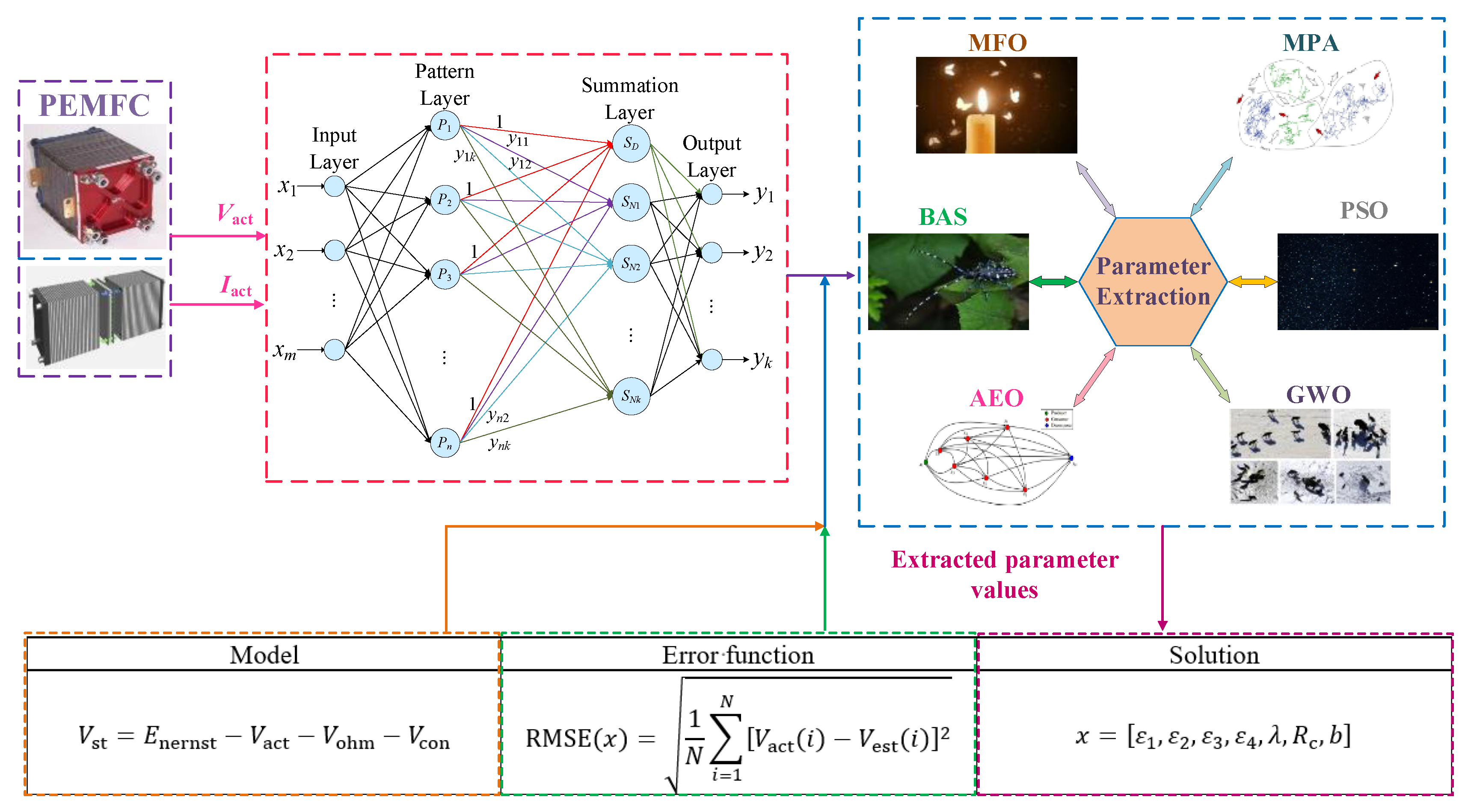
4. Case Studies

In this part, a GRNN and six typical MhAs were used to extract the parameters of the PEMFC model, respectively, moth fire optimization (MFO) [31], PSO [32], beetle antennae search (BAS) [33], grey wolf optimization (GWO) [34], marine predator algorithm (MPA) [35], and artificial ecosystem-based optimization (AEO). Then, the operating conditions were set up according to the actual working conditions of the cell, namely HTLP, MTMP, and LTHP. Due to the phenomenon of noise and insufficient available data, a GRNN was used to preprocess, de-noise and predict the 25 pairs of current and voltage data extracted from the cell. Finally, 145 sets of data were predicted and used for parameter identification research under multi-data. In this study, the parameters of PEMFC are shown in

Table 1. Model and algorithms parameter settings.

Types	Parameters	Value
PEMFC	PEM effective area	50.6 cm2
	PEM thickness	178 μm2
	Maximum iterations	500
Algorithms	Run times	10

.

Remark 1. 

The cell data in this study comes from experimental data provided by the cell manufacturer. The reason why a GRNN is used to process the V-I data of the PEMFC in this research is due to the inevitable impact of noise data in the measurement data. In addition, due to the loss of measured data, to verify the robustness of the GRNN applied to PEMFC parameter recognition, as well as the difficulty in measuring the V-I data of the PEMFC during actual operation, and due to battery aging and other phenomena, the difference between the measured data and the data from the battery factory is significant, which has a significant impact on the final parameter identification results.

4.1. GRNN for V-I Data Preprocessing

4.1.1. GRNN for V-I Data De-noising

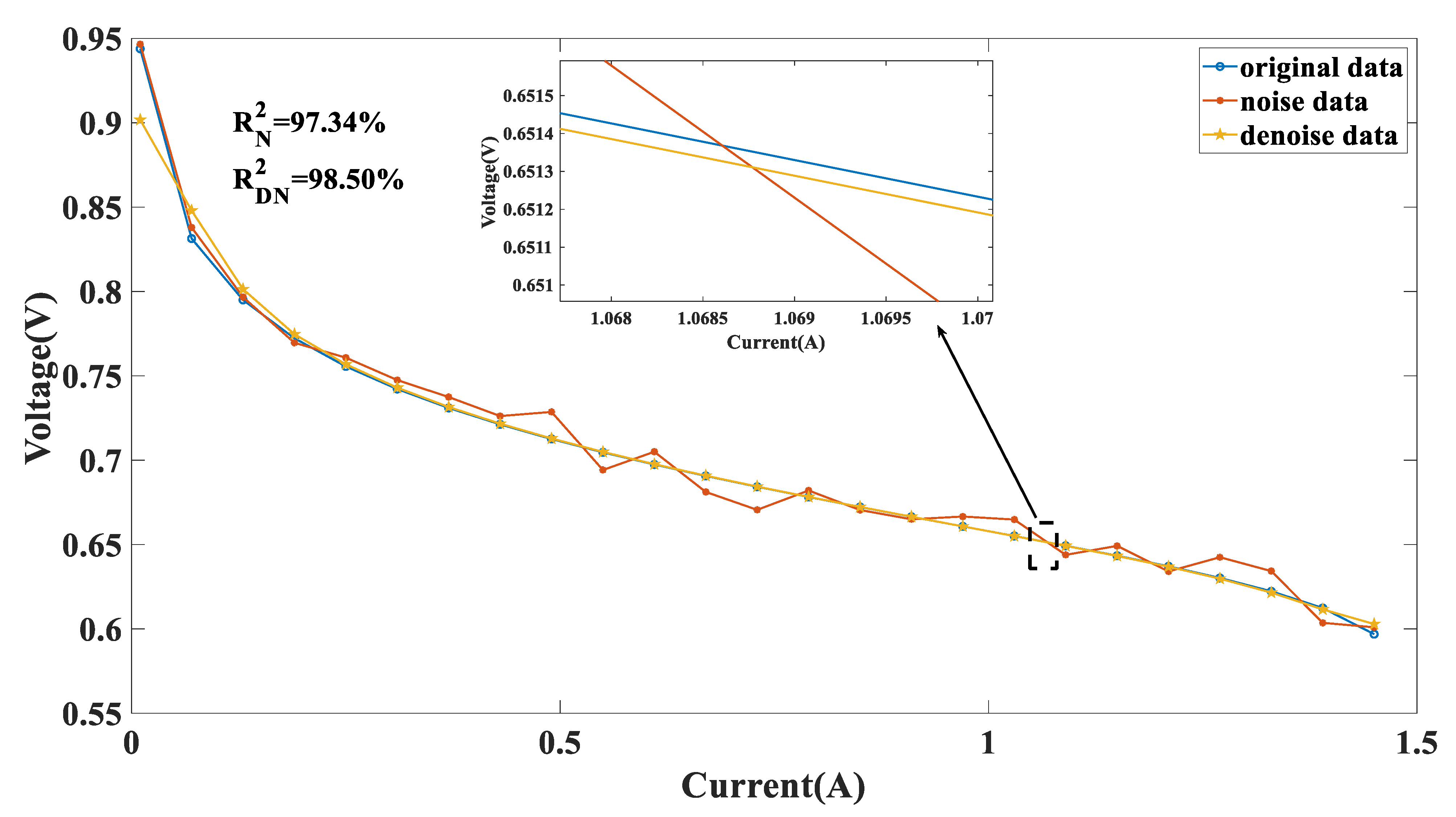
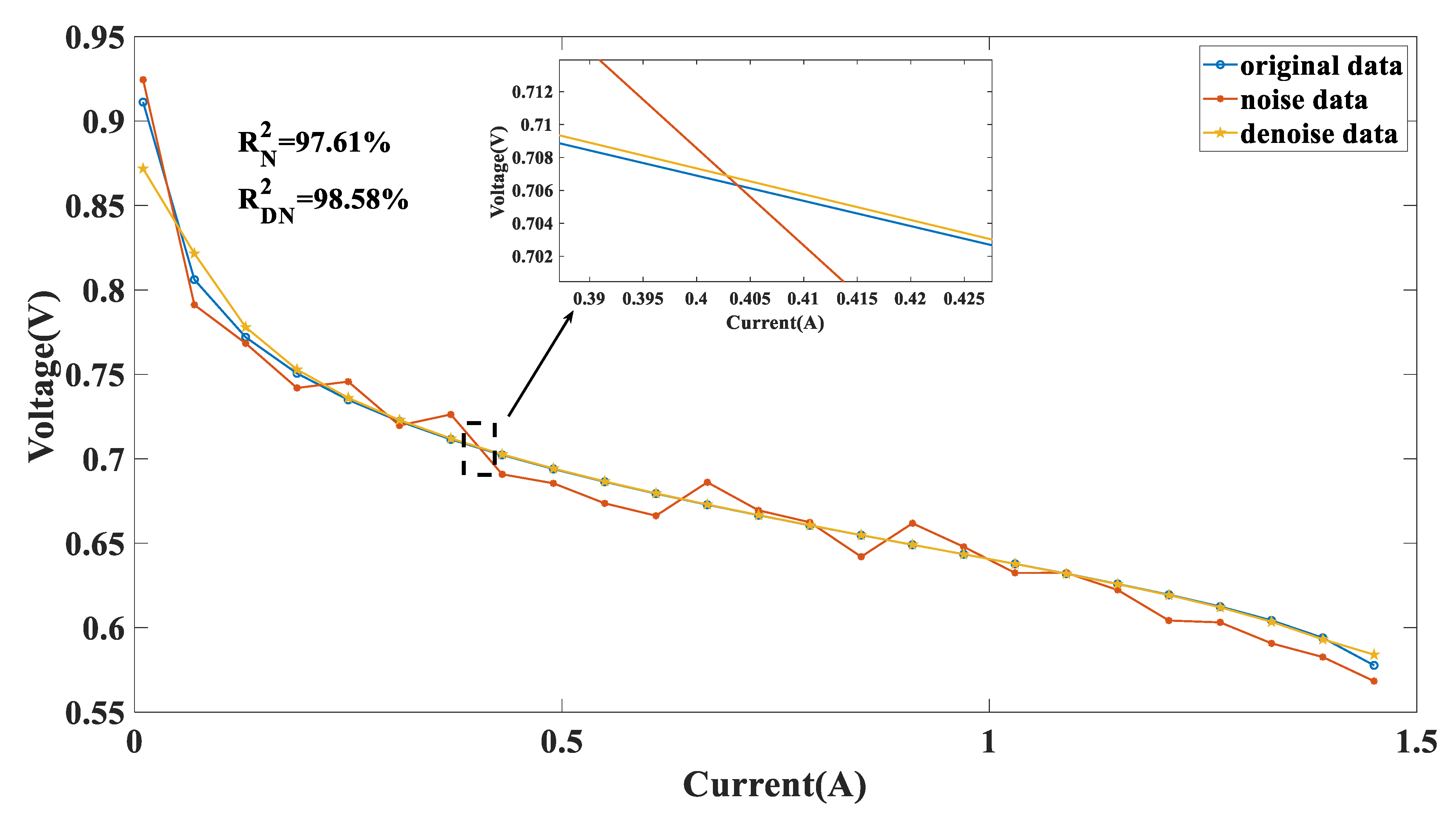
Small fluctuations may affect experimental data, similarly, the PEMFC is inevitably affected by noise when used in different environments. Undoubtedly, irregular changes in multiple variables can affect the inaccurate parameter identification of the PEMFC.

Therefore, to minimize the effect of the noise condition on the accuracy of the calculation results as much as possible, this paper adopts a GRNN [31]. The results obtained by de-noising the original data obtained under three operating conditions using the GRNN are shown in Figure 4, Figure 5 and Figure 6.

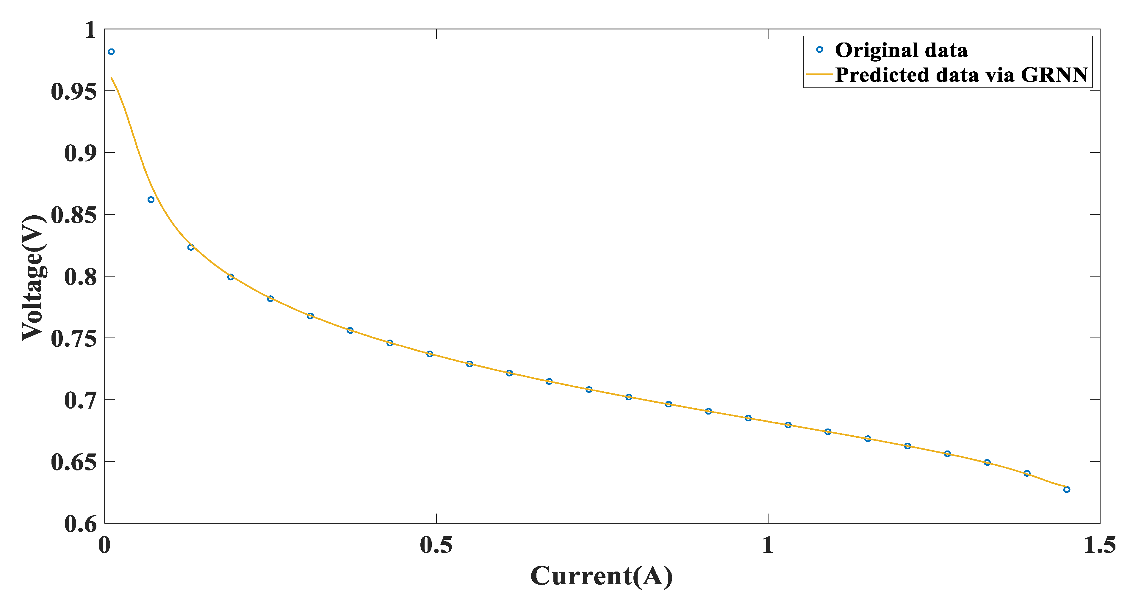
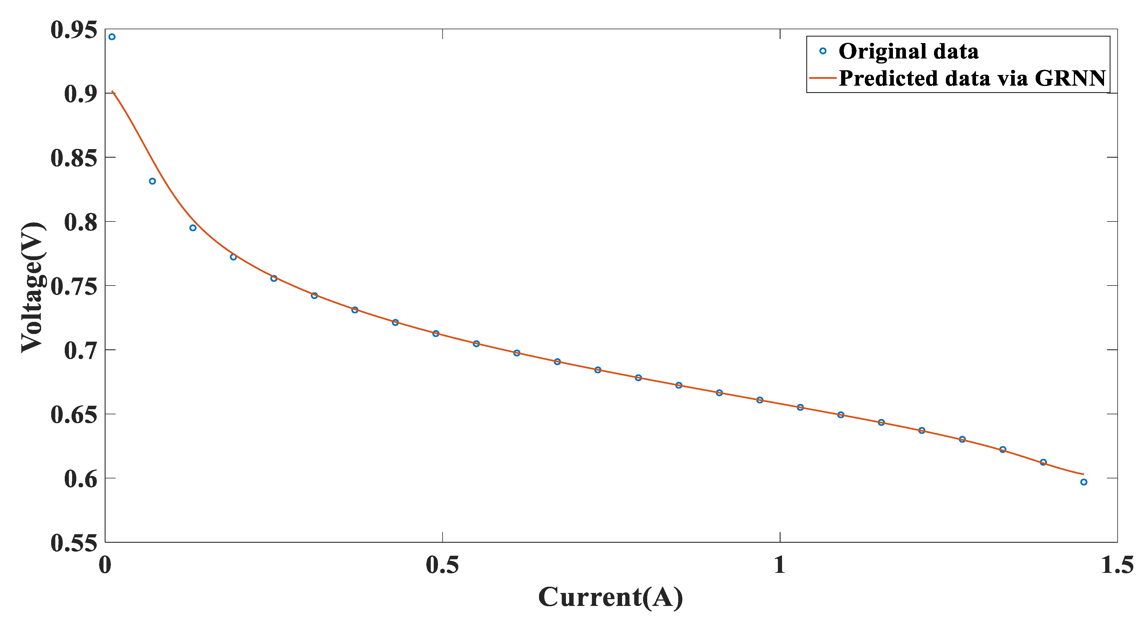
4.1.2. GRNN for V-I Data Prediction

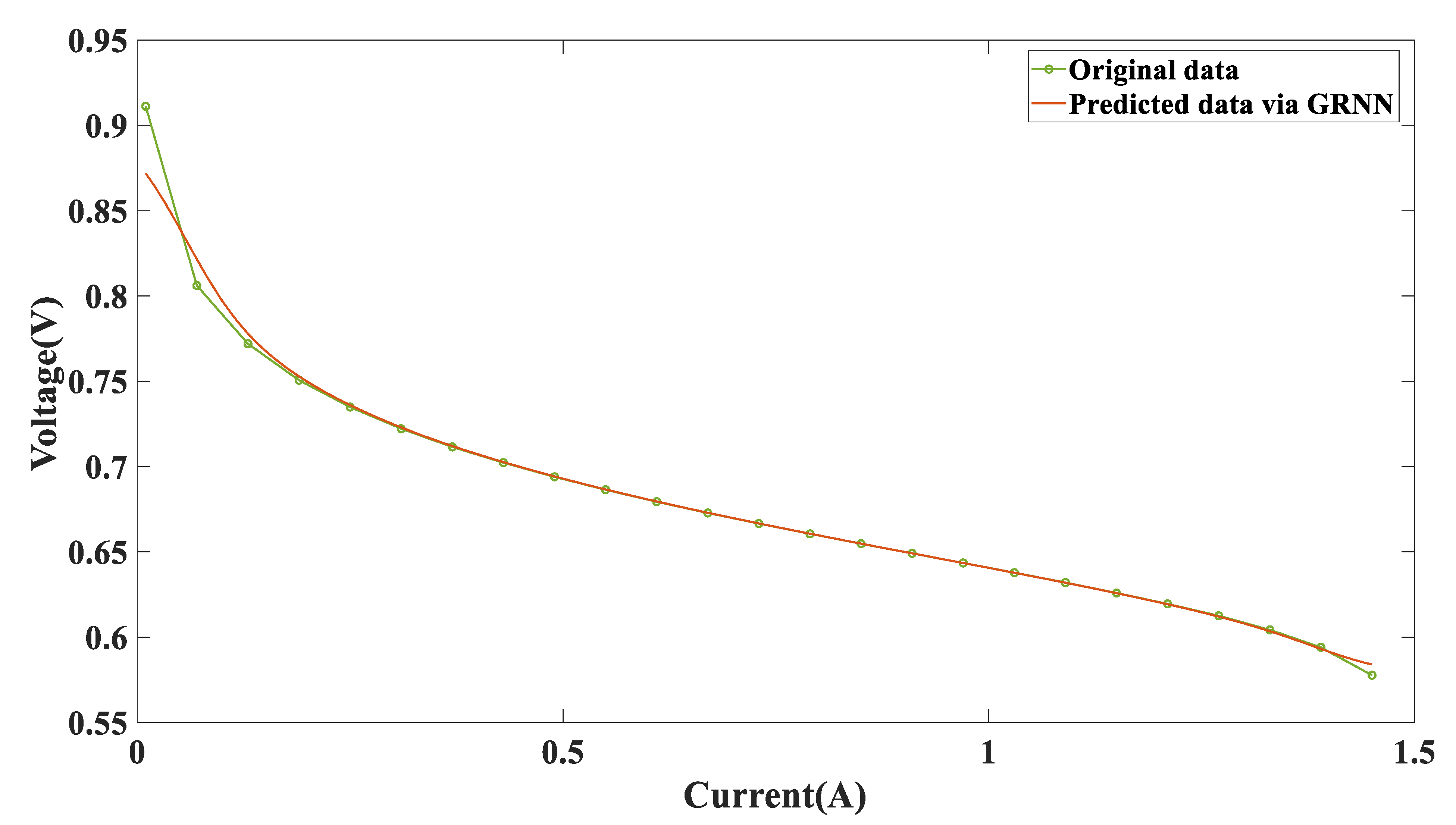
The parameter identification of PEMFC essentially relies on the most primitive current and voltage data, and the accuracy of the final identified parameters largely depends on the original data. However, actual data are difficult to obtain.

Therefore, this study uses existing data to train the GRNN model, then performs data prediction, expands the data volume, and improves the accuracy of identification parameters. The results obtained by data prediction of the original data obtained under three operating conditions using the GRNN are shown in Figure 7, Figure 8 and Figure 9.

4.2. PEMFC Parameter Extraction of HTLP

4.2.1. Noised Data

Table A1. Parameters identification results of noise data and de-noised data based under HTLP and MhAs.

State	Algorithms	Data	Identified Parameters							RMSE
			ԑ1	ԑ2	ԑ3	ԑ4	λ	Rc(Ω)	b(V)
HTLP	MPA	N	−0.9071	2.5000 × 10−3	3.6000 × 10−5	−1.0000 × 10−4	23.0000	1.0000 × 10−4	0.0136	8.2100 × 10−3
		DN	−0.9437	3.4000 × 10−3	9.8000 × 10−5	−1.0000 × 10−4	13.5231	8.0000 × 10−4	0.0136	1.4792 × 10−3
	AEO	N	−0.9384	2.5000 × 10−3	3.6000 × 10−5	−1.0000 × 10−4	18.1835	1.0000 × 10−4	0.0136	8.2182 × 10−3
		DN	−0.9142	2.8000 × 10−3	6.1300 × 10−5	−1.5836 × 10−4	13.4758	8.0000 × 10−4	0.0136	1.4798 × 10−3
	PSO	N	−0.9610	2.9000 × 10−3	3.6000 × 10−5	−2.6000 × 10−4	17.8012	1.0000 × 10−4	0.0220	8.3356 × 10−2
		DN	−0.9882	3.0000 × 10−3	3.6000 × 10−5	−2.6000 × 10−4	14.1474	1.0000 × 10−4	0.0693	4.2543 × 10−2
	BAS	N	−1.0078	3.2000 × 10−3	5.5900 × 10−5	−1.6467 × 10−4	17.2423	1.5174 × 10−4	0.0217	3.8371 × 10−2
		DN	−0.9756	3.0000 × 10−3	7.1700 × 10−5	−1.1658 × 10−4	13.9875	2.4255 × 10−4	0.0156	2.2016 × 10−2
	GWO	N	−0.8561	2.7000 × 10−3	6.1100 × 10−5	−1.7406 × 10−4	19.4860	6.5726 × 10−4	0.0136	8.3379 × 10−3
		DN	−0.8714	2.8000 × 10−3	7.0143 × 10−5	−1.5764 × 10−4	11.3971	4.8605 × 10−4	0.0136	1.5914 × 10−3
	MFO	N	−0.9520	2.7000 × 10−3	4.3300 × 10−5	−1.7414 × 10−4	23.0000	8.0000 × 10−4	0.0136	8.2942 × 10−3
		DN	−0.8531	3.1000 × 10−3	9.3100 × 10−5	−1.5858 × 10−4	12.7877	1.0000 × 10−4	0.0136	1.5251 × 10−3

of Appendix A shows the statistics of the results of parameter extraction of noise and noise reduction data, respectively, by six algorithms under HTLP, where the symbol ‘N’ denotes the results obtained from noised data and ‘DN’ denotes the results obtained from de-noised data. From Table A1 of Appendix A, it is obvious that after data noise reduction, the RMSE is lower than that obtained from noised data. After data noise reduction, the RMSE of the PSO algorithm and the BAS algorithm has a magnitude of the minus second power of ten, while the RMSE of the other four algorithms has a magnitude of the minus third power of ten. The MPA algorithm exhibits the most significant decrease of 82.10%, whereas the BAS algorithm demonstrates a comparatively smaller reduction of 42.62%.

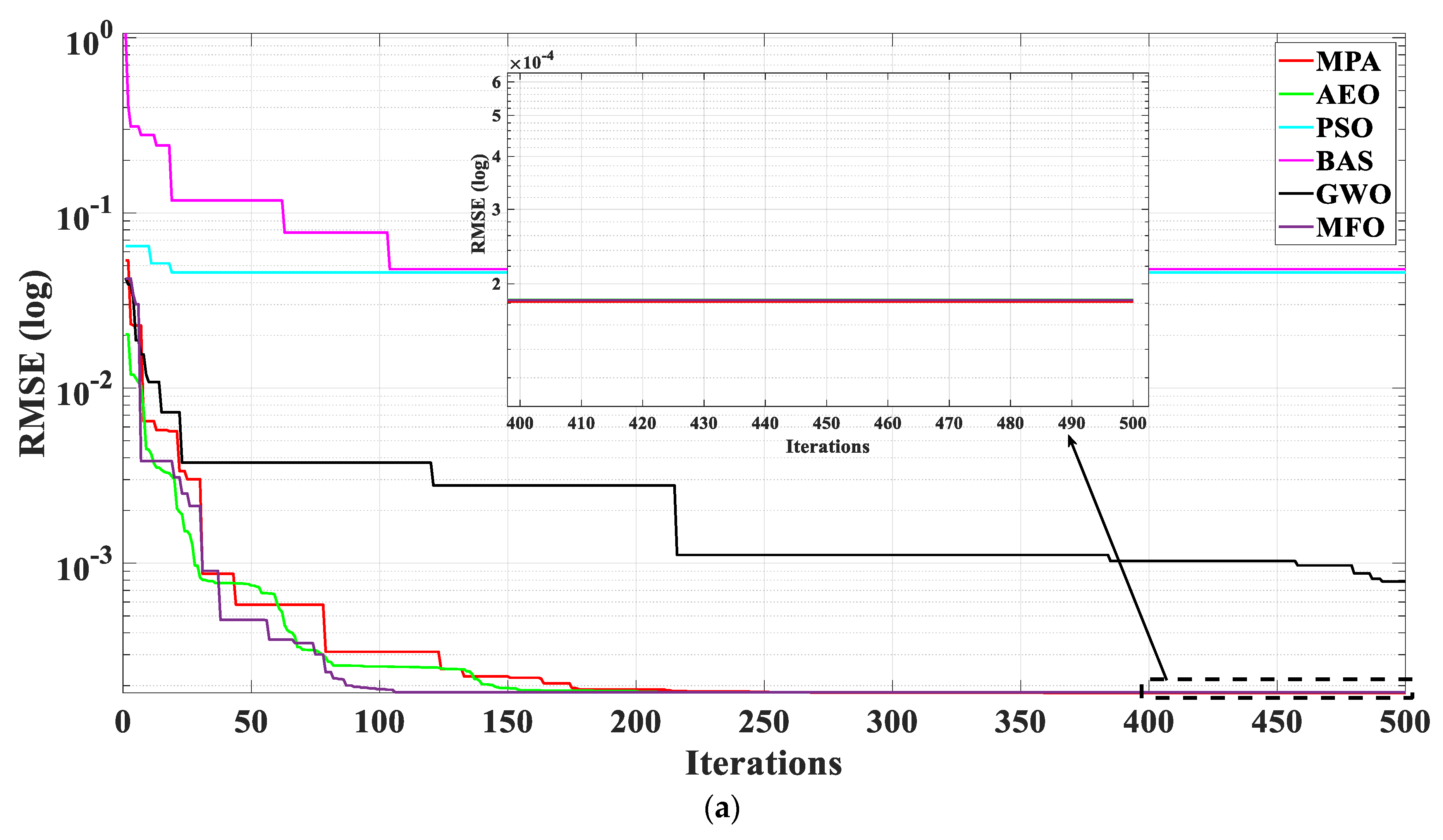
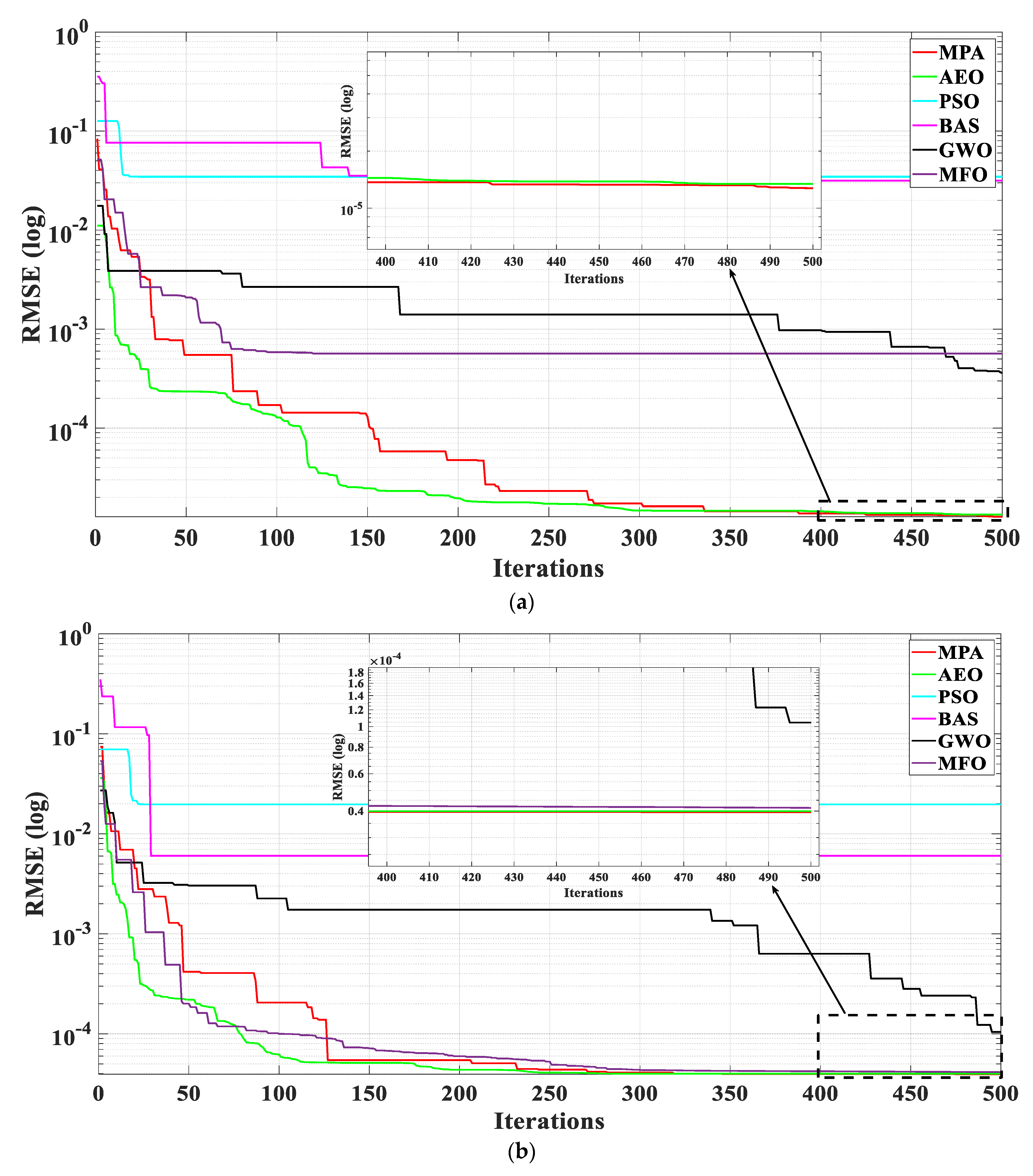
In addition, Figure 10 shows the RMSE convergence curves obtained by six algorithms trained on two datasets. The results obtained based on data de-noising have smaller errors than those obtained from noised data. The special process is that the RMSE obtained by six algorithms on de-noised data is lower than that obtained from noised data.

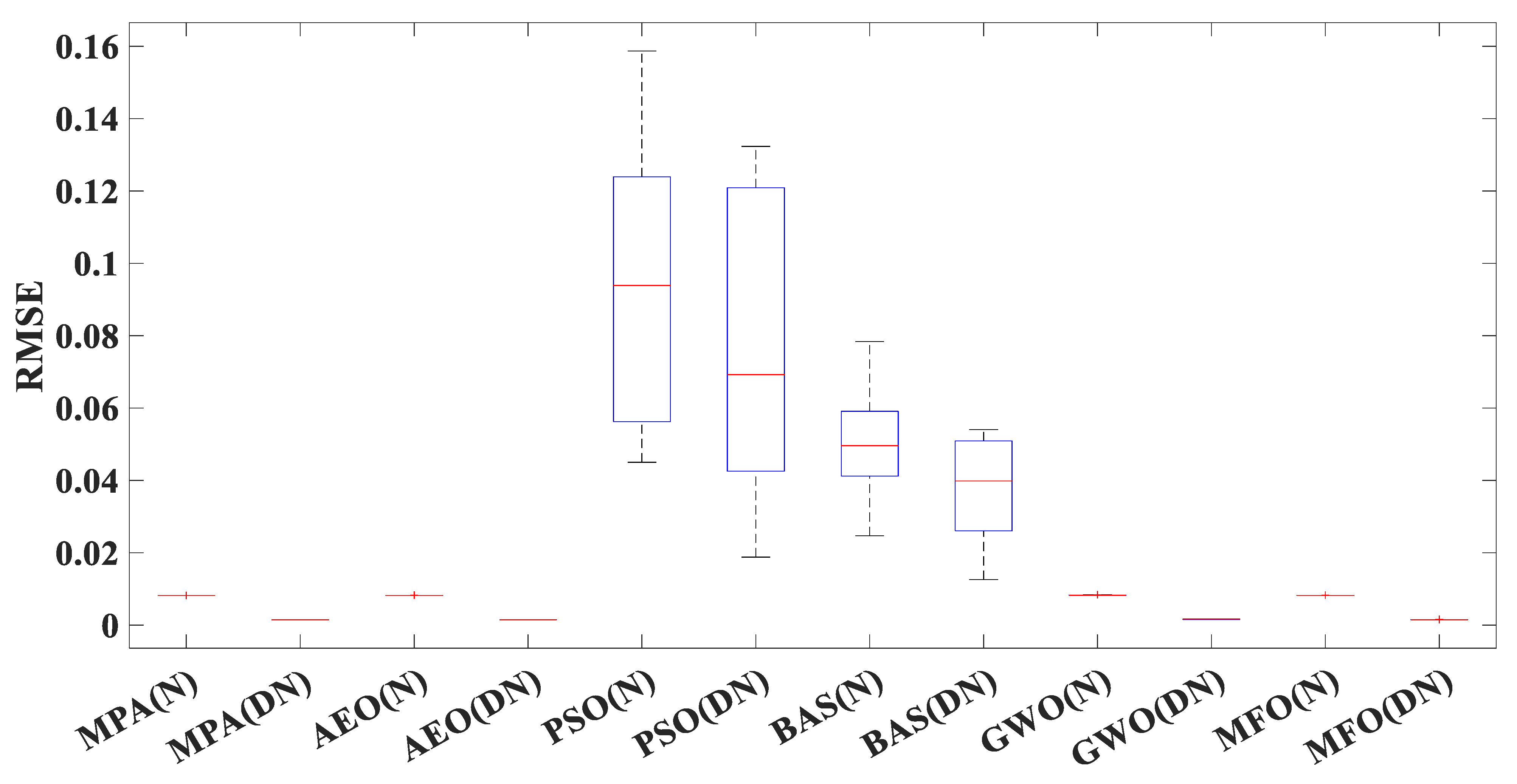
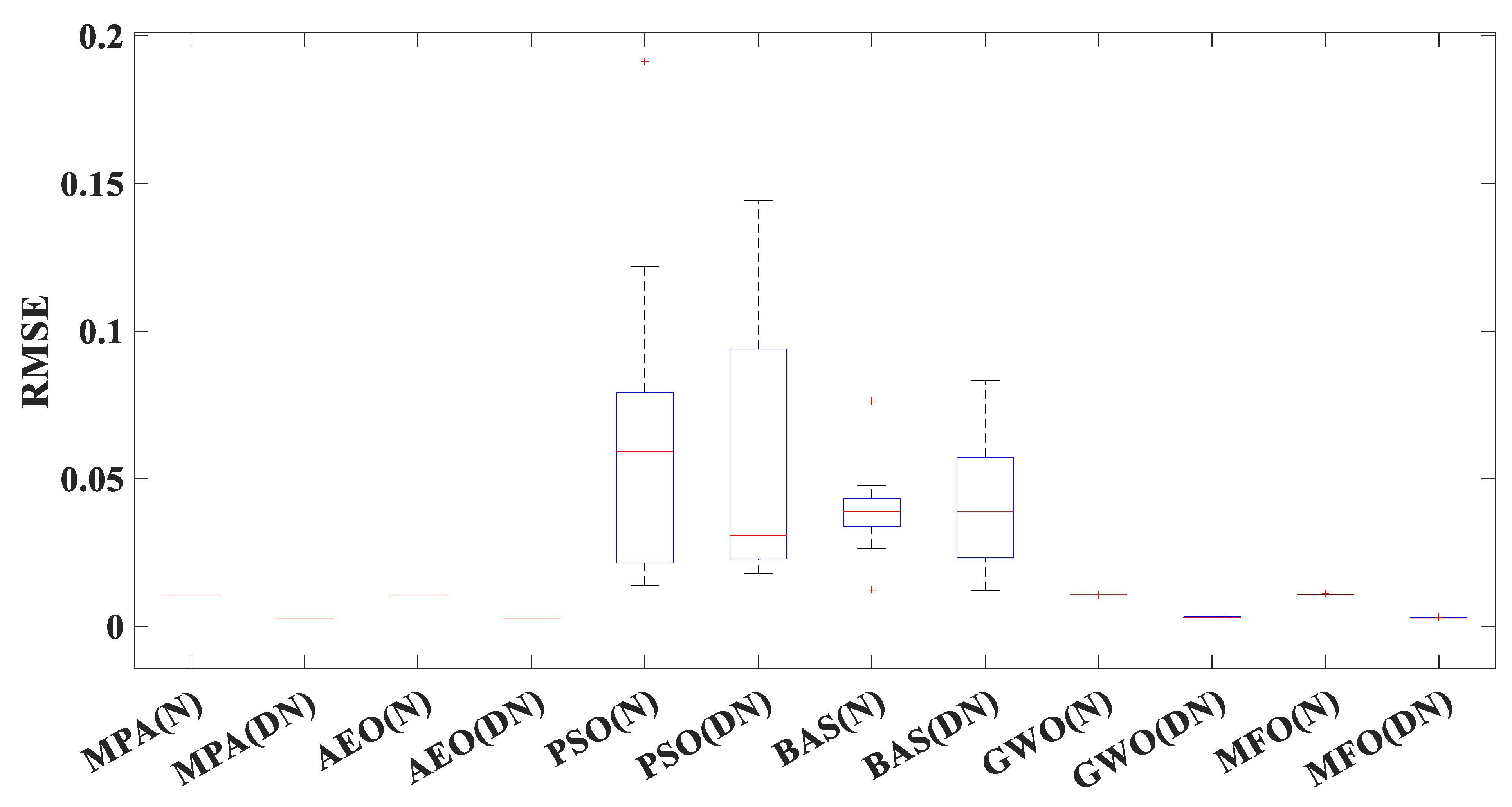
In order to acquire the visual impact of the two different training data, the boxplot illustrates the distribution of RMSE obtained by MhAs which is presented in Figure 11. It can be seen from the figure that after data de-noising, the RMSE corresponding to each algorithm in the boxplot decreased to a certain extent. However, after data de-noising, the upper and low bounds of the boxplot of PSO and BAS changed significantly, shrinking toward the RMSE median. In addition, MPA, AEO, GWO, and MFO have superior performance compared with other algorithms. This fully shows that GRNN data noise reduction can improve the stability of MhAs in parameter identification.

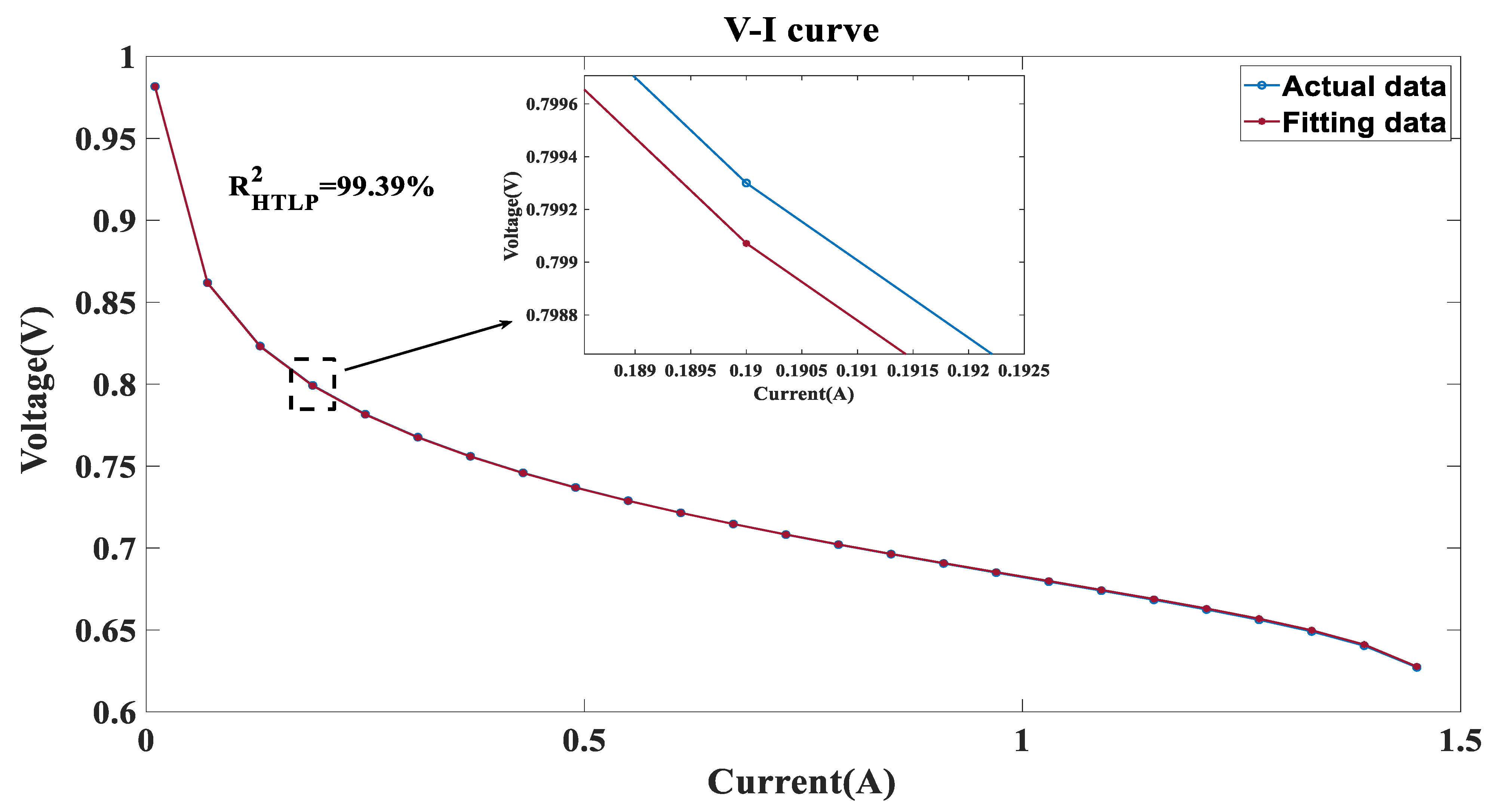
Figure 12 presents the V-I characteristic curves based on high-temperature and low-pressure obtained by the GRNN fitting the MPA algorithm under noise reduction data conditions. It can be seen that the curve of fitting data almost coincides with the curve of actual data and the error measured by RMSE is equal to 99.39%, which demonstrates the parameter identification effect is in line with expectations.

4.2.2. Insufficient Data

Table A2. Parameters identification results of original data and predicted data based under HTLP and MhAs.

State	Algorithms	Data	Identified Parameters							RMSE
			ԑ1	ԑ2	ԑ3	ԑ4	λ	Rc(Ω)	b(V)
HTLP	MPA	O	−0.9788	2.6836 × 10−3	3.6000 × 10−5	−1.7361 × 10−4	23.0000	1.0000 × 10−4	0.0136	1.8172 × 10−4
		P	−0.9040	2.4849 × 10−3	3.6873 × 10−5	−1.7361 × 10−4	23.0000	3.2975 × 10−4	0.0136	1.2978 × 10−4
	AEO	O	−1.0234	3.3728 × 10−3	7.4400 × 10−5	−1.7358 × 10−4	22.9704	1.0000 × 10−4	0.0136	1.8329 × 10−4
		P	−0.9936	3.0606 × 10−3	5.8834 × 10−5	−1.7361 × 10−4	22.9999	3.0556 × 10−4	0.0136	1.2979 × 10−4
	PSO	O	−0.9918	2.9998 × 10−3	5.3800 × 10−5	−1.8100 × 10−4	20.4025	2.9781 × 10−4	0.0136	4.5757 × 10−2
		P	−0.9975	3.1380 × 10−3	6.0205 × 10−5	−1.0567 × 10−4	21.0376	7.1037 × 10−4	0.1105	7.1117 × 10−2
	BAS	O	−0.9646	2.7871 × 10−3	4.7900 × 10−5	−1.2795 × 10−4	11.8778	7.2134 × 10−4	0.0315	4.7789 × 10−2
		P	−1.0520	3.2208 × 10−3	6.9550 × 10−5	−1.1996 × 10−4	16.9202	1.0746 × 10−4	0.0233	2.4037 × 10−2
	GWO	O	−1.0150	3.3641 × 10−3	7.5400 × 10−5	−1.7248 × 10−4	14.8613	1.8872 × 10−4	0.0136	7.8535 × 10−4
		P	−1.1592	3.9697 × 10−3	8.8869 × 10−5	−1.7324 × 10−4	21.1633	2.9474 × 10−4	0.0137	2.6180 × 10−4
	MFO	O	−0.8531	2.5174 × 10−3	4.9000 × 10−5	−1.7360 × 10−4	23.0000	1.0000 × 10−4	0.0136	1.8301 × 10−4
		P	−0.8539	3.2393 × 10−3	9.8000 × 10−5	−1.7361 × 10−4	23.0000	2.6234 × 10−4	0.0136	1.2979 × 10−4

of Appendix A shows the statistics of the results of parameter extraction of insufficient and predicted data, respectively, by six algorithms under HTLP, where the symbol ‘O’ denotes the source data and ‘P’ denotes the predicted data. From Table A2 of Appendix A, it can be obtained by observation that after data prediction, the RMSE achieved by the five algorithms is lower than that obtained from predicted data, except for PSO algorithm. After data prediction, the RMSE of the PSO algorithm and the BAS algorithm has a magnitude of the minus second power of ten, while the RMSE of the other four algorithms has a magnitude of the minus fourth power of ten. The GWO algorithm exhibits the most significant decrease of 66.66%, whereas the MPA algorithm demonstrates a comparatively smaller reduction of 28.58%.

Figure 13 describes the RMSE convergence curves obtained by six algorithms on two datasets, with most algorithms having lower RMSE obtained from predicted data, and only RMSE based on multi-data of PSO being larger than RMSE based on low data. In addition, compared with other algorithms, MPA, AEO, and MFO can quickly acquire a smaller RMSE and have great stability.

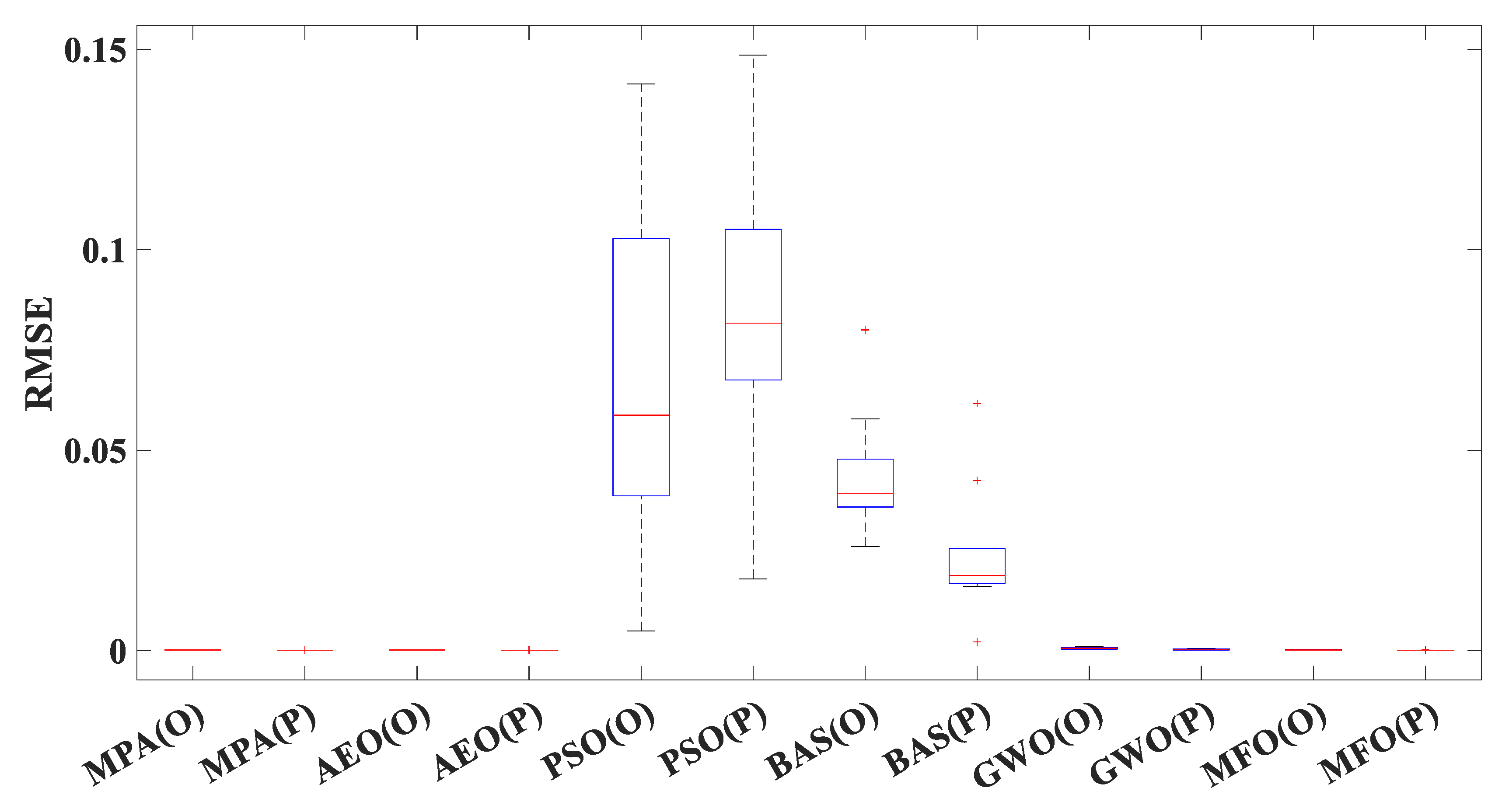
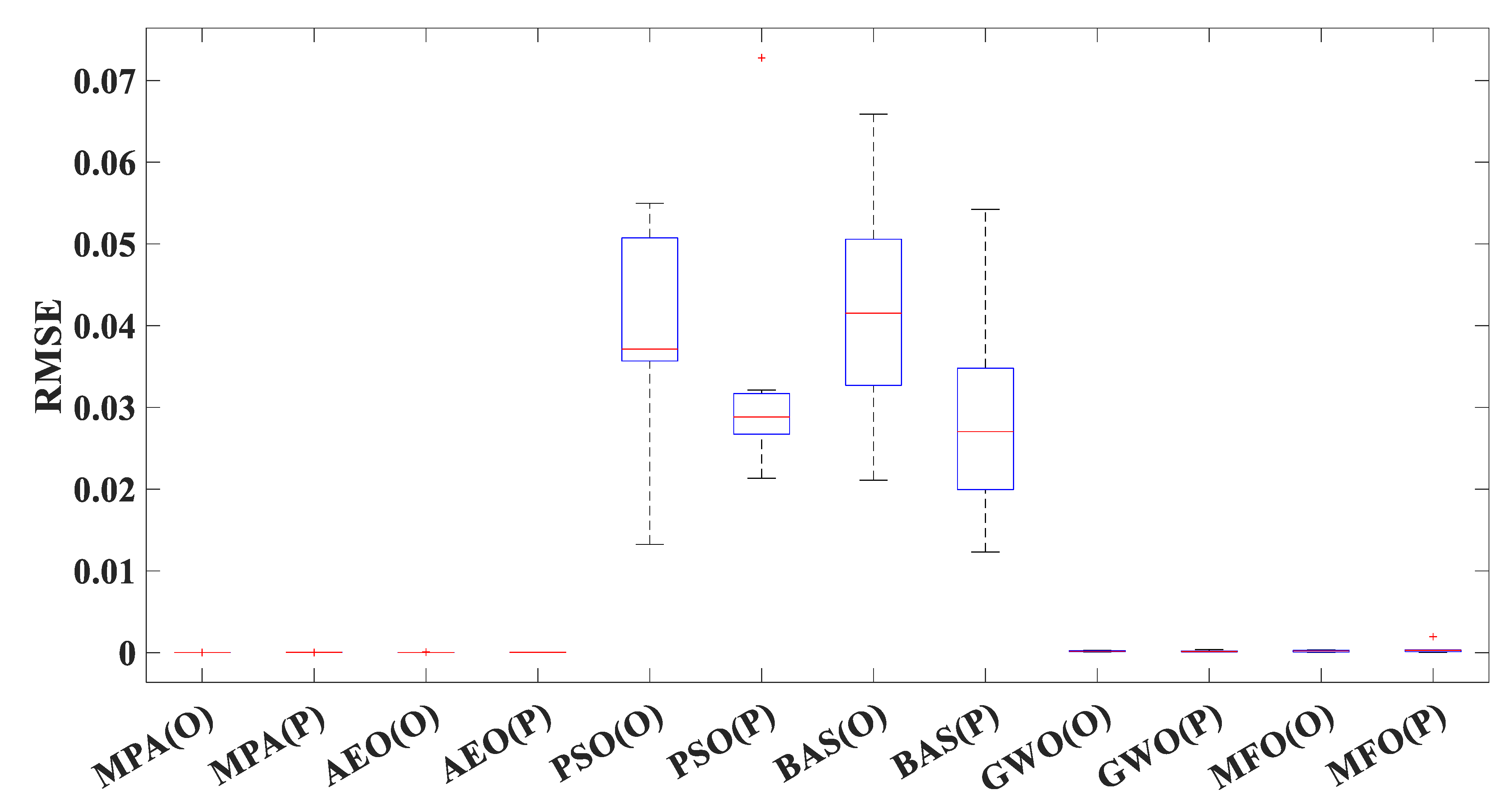
The boxplot illustrates the distribution of RMSE obtained by MhAs which is presented in Figure 14. It can be obtained by observation that except for the PSO, the RMSE obtained based on predicted data are lower than the RMSE obtained from original data. On the contrary, the RMSE of PSO has increased. In addition, MPA, AEO, GWO, and MFO have superior performance compared with other algorithms.

4.3. PEMFC Parameter Extraction of MTMP

4.3.1. Noised Data

Table A3. Parameters identification results of noise data and de-noised data based under MTMP and MhAs.

State	Algorithms	Data	Identified Parameters							RMSE
			ԑ1	ԑ2	ԑ3	ԑ4	λ	Rc(Ω)	b(V)
MTMP	MPA	N	−0.9356	2.5684 × 10−3	3.6000 × 10−5	−1.7905 × 10−4	23.0000	1.0000 × 10−4	0.0136	9.0391 × 10−3
		DN	−0.9416	3.3689 × 10−3	9.8000 × 10−5	−1.4121 × 10−4	10.0000	8.0000 × 10−4	0.0149	3.0236 × 10−3
	AEO	N	−1.0197	3.0243 × 10−3	5.0100 × 10−5	−1.7902 × 10−4	22.9999	1.1388 × 10−4	0.0136	9.0398 × 10−3
		DN	−0.9375	2.5467 × 10−3	4.1900 × 10−5	−1.4125 × 10−4	10.0000	8.0000 × 10−4	0.0149	3.0294 × 10−3
	PSO	N	−0.9882	3.0804 × 10−3	3.6000 × 10−5	−2.6000 × 10−4	14.1474	1.0000 × 10−4	0.0693	5.0083 × 10−2
		DN	−0.9547	3.3380 × 10−3	9.8000 × 10−5	−9.5400 × 10−5	13.7242	8.0000 × 10−4	0.0292	2.3422 × 10−2
	BAS	N	−0.9699	3.0822 × 10−3	8.2000 × 10−5	−9.9500 × 10−5	19.7473	4.3042 × 10−4	0.0369	2.5185 × 10−2
		DN	−0.9584	2.7603 × 10−3	4.5600 × 10−5	−1.7596 × 10−4	11.8635	7.0335 × 10−4	0.0272	1.8866 × 10−2
	GWO	N	−1.1160	3.7093 × 10−3	7.7473 × 10−5	−1.7869 × 10−4	22.9456	6.0307 × 10−4	0.0136	9.1580 × 10−3
		DN	−1.0319	2.8337 × 10−3	4.2200 × 10−5	−1.4112 × 10−4	10.0000	4.7206 × 10−4	0.0151	3.0655 × 10−3
	MFO	N	−0.9990	3.1232 × 10−3	6.1200 × 10−5	−1.7904 × 10−4	23.0000	1.0000 × 10−4	0.0136	9.0445 × 10−3
		DN	−1.1997	3.5568 × 10−3	5.7400 × 10−5	−1.4348 × 10−4	10.0000	1.0000 × 10−4	0.0136	3.4203 × 10−3

of Appendix A shows the statistics of the results of parameter extraction of noise and noise reduction data, respectively, by six algorithms under MTMP. From Table A3 of Appendix A, it can be seen that after data noise reduction, the RMSE obtained by the six algorithms is lower than that obtained from noised data. After data noise reduction, the RMSE of the PSO algorithm and the BAS algorithm has a magnitude of the minus second power of ten, while the RMSEs of the other third algorithms have a magnitude of the minus third power of ten. The GWO algorithm exhibits the most significant decrease of 66.53%, whereas the BAS algorithm demonstrates a comparatively smaller reduction of 25.09%.

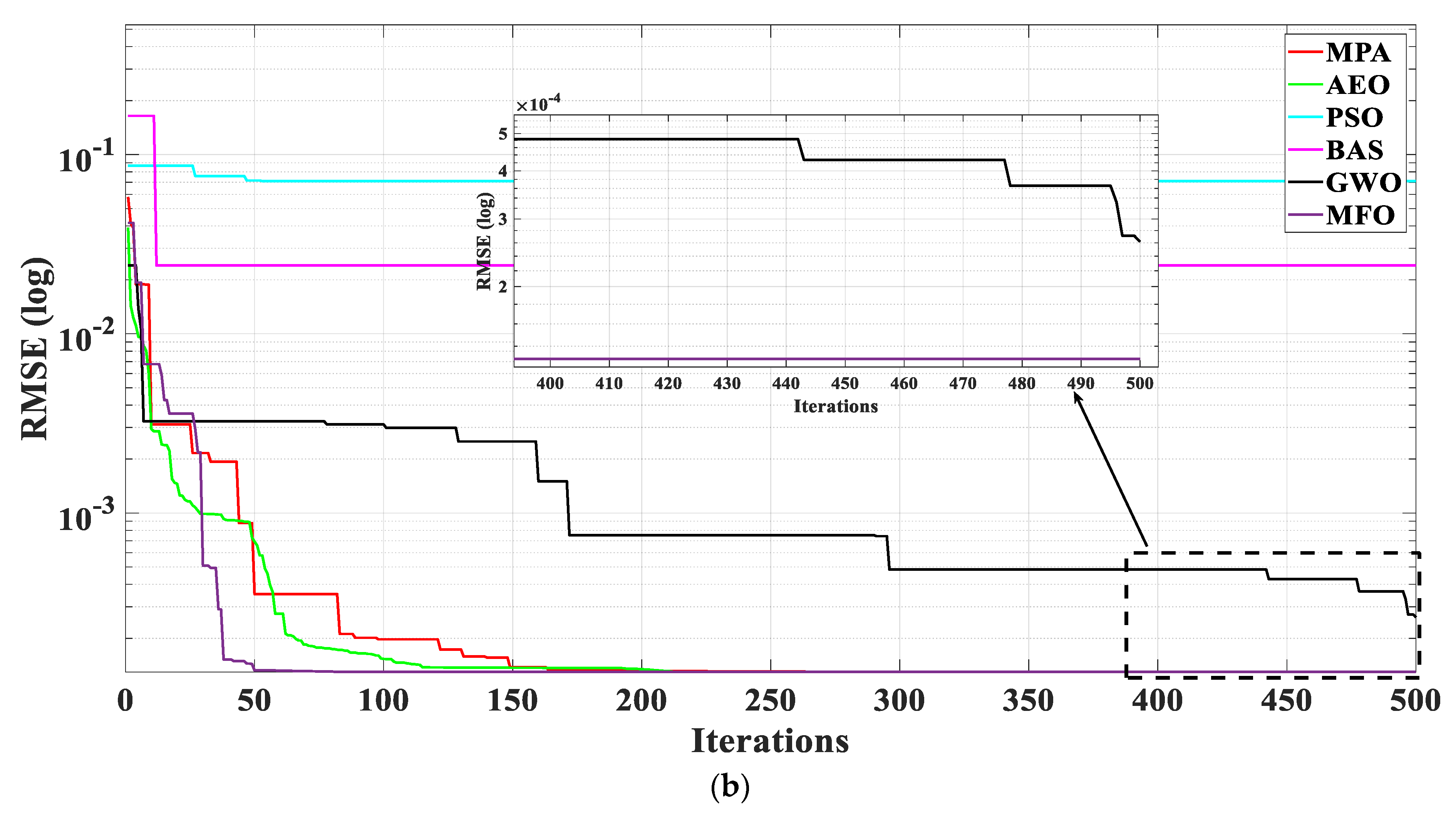
Figure 15 describes the RMSE convergence curves obtained by six algorithms under noise and noise reduction data conditions. It can be obtained by observation that the RMSE based on de-noised data of parameter identification results has decreased. The special process is that the RMSE obtained by six algorithms on de-noised data is lower than that obtained from noised data.

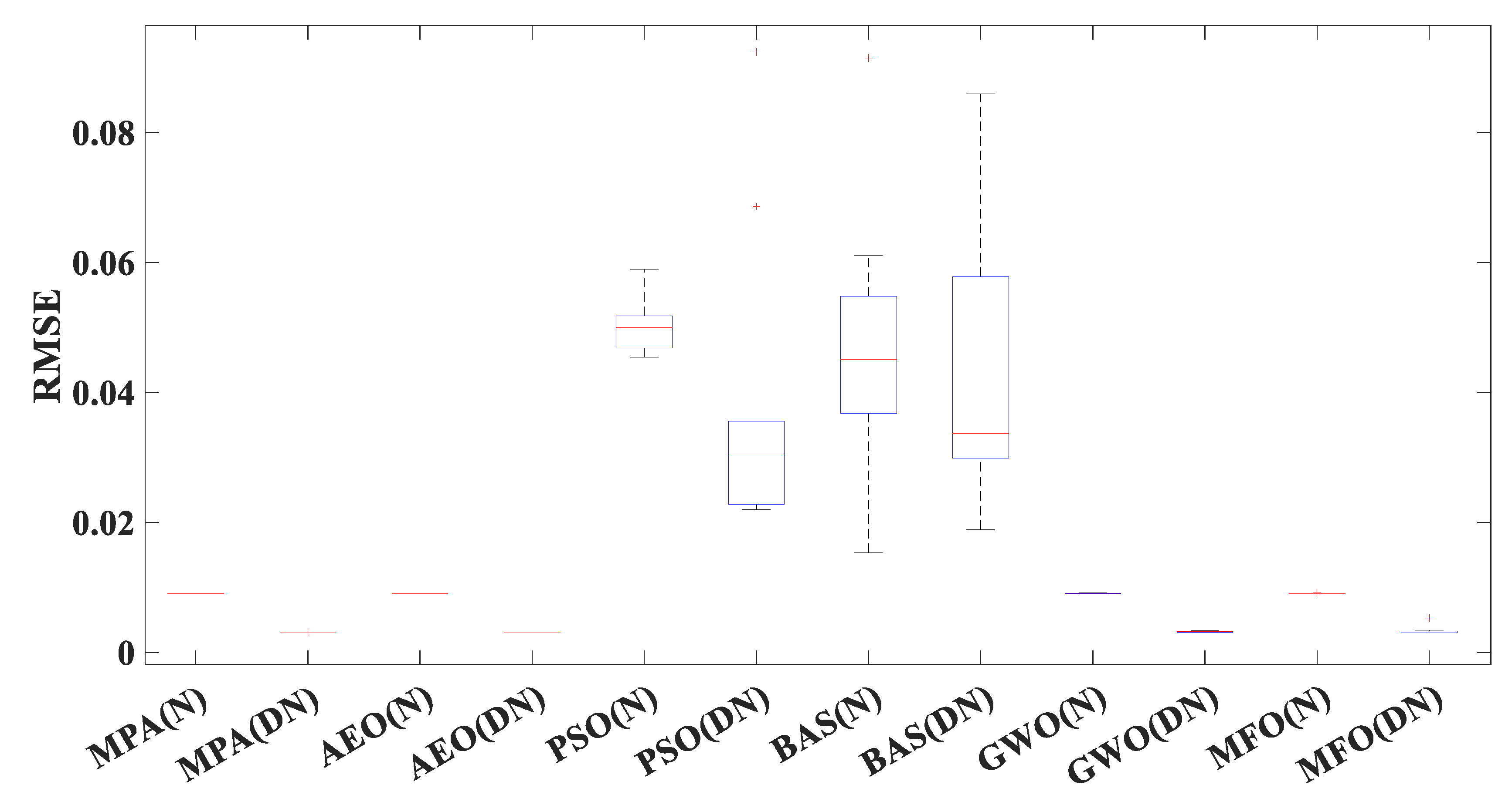
Figure 16 describes the RMSE distribution boxplot obtained by six algorithms. It can be obtained by observation that except for the BAS, the RMSE obtained from predicted data has decreased. On the contrary, the upper and low bounds of BAS have increased. Also, there are a few outliers in the boxplot of MFO and PSO. In addition, MPA, AEO, and GWO have superior performance compared with other algorithms. This fully shows that GRNN data noise reduction can improve the stability of MhAs in parameter identification.

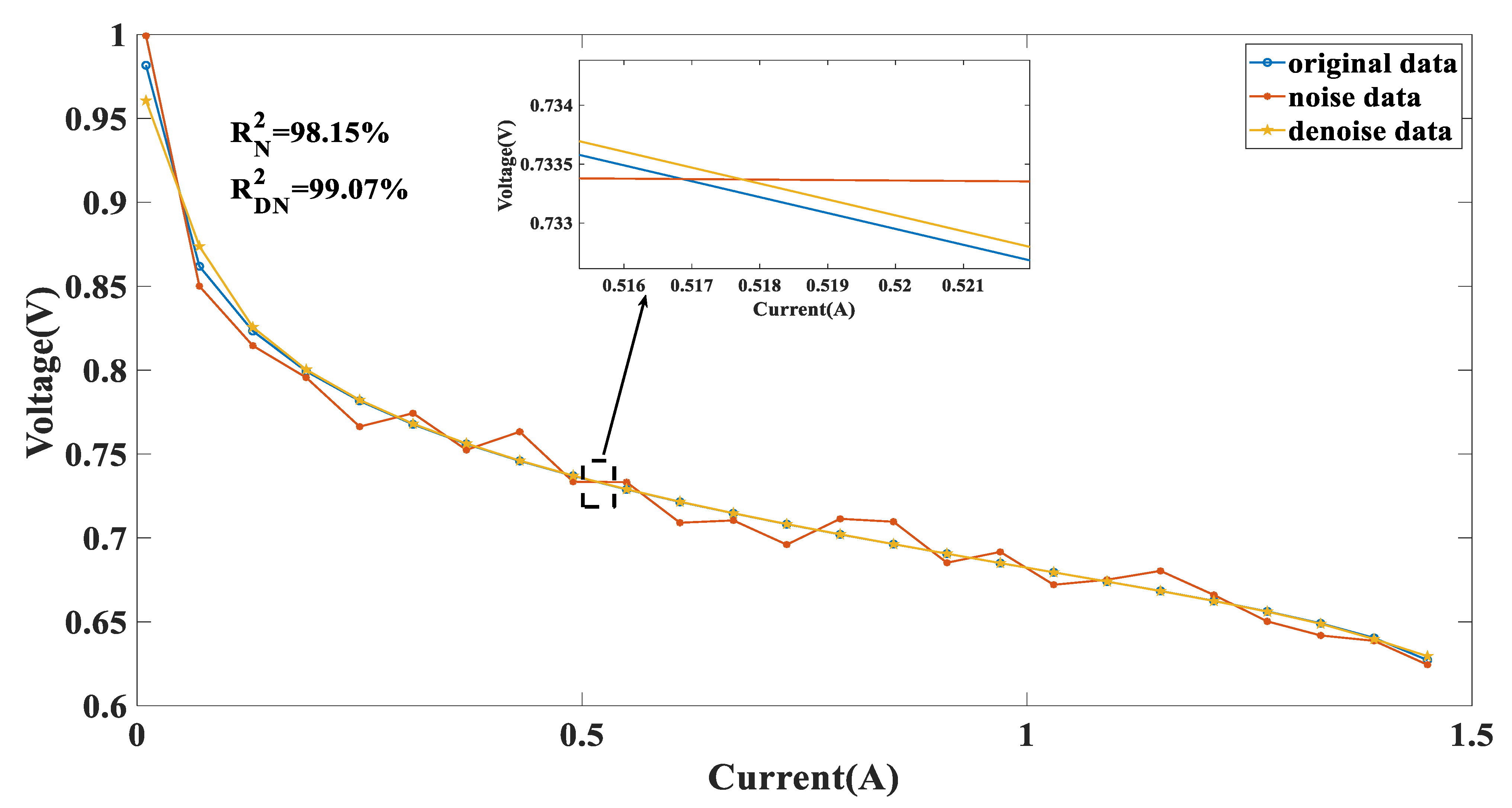
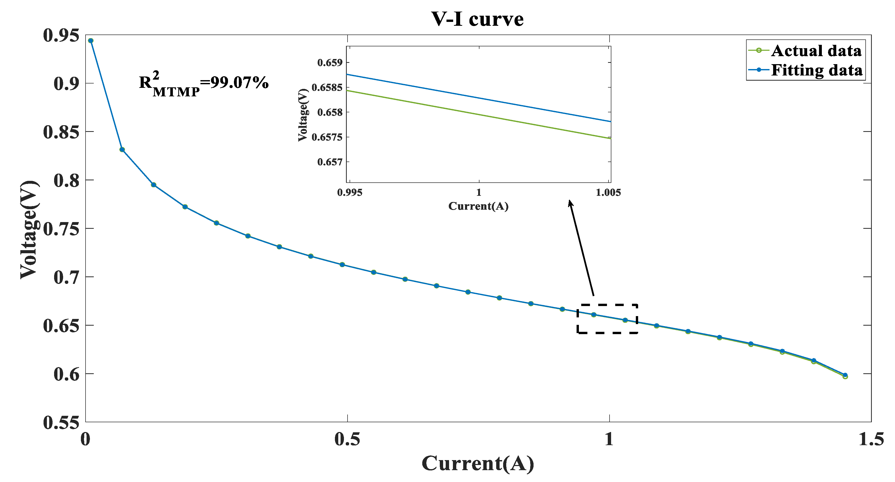
Figure 17 presents the V-I characteristic curves based on medium-temperature and medium-pressure obtained by the GRNN fitting the GWO algorithm under noise reduction data conditions. It can be obtained by observation that the curve of fitting data almost coincides with the curve of actual data and the error measured by RMSE is equal to 99.07%, which demonstrates the parameter identification effect is in line with expectations.

4.3.2. Insufficient Data

Table A4. Parameters identification results of original data and predicted data based under MTMP and MhAs.

State	Algorithms	Data	Identified Parameters							RMSE
			ԑ1	ԑ2	ԑ3	ԑ4	λ	Rc(Ω)	b(V)
MTMP	MPA	O	−0.9872	3.6025 × 10−3	9.7600 × 10−5	−1.7220 × 10−4	16.5370	7.9936 × 10−4	0.0158	7.2400 × 10−6
		P	−0.8886	3.3117 × 10−3	9.8000 × 10−5	−1.7224 × 10−4	17.0972	7.9999 × 10−4	0.0158	2.6500 × 10−6
	AEO	O	−0.8531	2.9435 × 10−3	7.9900 × 10−5	−1.7234 × 10−4	19.3780	8.0000 × 10−4	0.0161	6.8300 × 10−5
		P	−1.0941	3.8739 × 10−3	9.4200 × 10−5	−1.7224 × 10−4	17.0795	8.0000 × 10−4	0.0158	3.1200 × 10−5
	PSO	O	−0.9523	3.3678 × 10−3	9.8000 × 10−5	−9.5400 × 10−5	18.0146	8.0000 × 10−4	0.0373	1.8500 × 10−2
		P	−1.0564	3.5663 × 10−3	9.8000 × 10−5	−9.5400 × 10−5	21.0946	8.0000 × 10−4	0.0174	2.1842 × 10−2
	BAS	O	−0.9972	3.5814 × 10−3	9.2100 × 10−5	−1.2458 × 10−4	19.1842	1.6857 × 10−4	0.0408	2.9545 × 10−2
		P	−0.9651	3.3046 × 10−3	9.2400 × 10−5	−1.2678 × 10−4	18.4227	7.8429 × 10−4	0.0436	2.5628 × 10−2
	GWO	O	−0.9400	2.5785 × 10−3	3.6500 × 10−5	−1.7195 × 10−4	10.1534	1.0110 × 10−4	0.0137	2.6819 × 10−4
		P	−0.9093	2.8226 × 10−3	5.9800 × 10−5	−1.7183 × 10−4	11.3025	3.9408 × 10−4	0.0142	2.2363 × 10−4
	MFO	O	−0.9032	2.4639 × 10−3	3.6300 × 10−5	−1.7252 × 10−4	23.0000	8.0000 × 10−4	0.0163	1.2940 × 10−4
		P	−0.8551	3.0497 × 10−3	8.6800 × 10−5	−1.7204 × 10−4	10.3446	1.0000 × 10−4	0.0136	2.8621 × 10−4

of Appendix A shows the statistics of the results of parameter extraction of insufficient and predicted data, respectively, by six algorithms under MTMP. From Table A4 of Appendix A, it is obvious that by data prediction, the RMSE obtained by the four algorithms is lower than that obtained from predicted data, except for the MFO and PSO algorithms. After data prediction, the RMSE of the PSO algorithm and the BAS algorithm has a magnitude of the minus second power of ten, while the RMSE of other algorithms has a magnitude exceeding the minus fourth power of ten. The MPA algorithm exhibits the most significant decrease of 63.40%, whereas the BAS algorithm demonstrates a comparatively smaller reduction of 13.26%.

Figure 18 describes the RMSE convergence curves obtained by six algorithms on two datasets, with most algorithms having lower RMSE based on predicted data, and only RMSE based on prediction data of BAS and PSO being larger than RMSE based on low data. In addition, compared with other algorithms, MPA and AEO can quickly acquire a smaller RMSE and have great stability.

Figure 19 describes the RMSE distribution boxplot obtained by six algorithms. It can be obtained by observation that the RMSE obtained based on predicted data has decreased. In addition, MPA has superior performance compared with other algorithms. This fully shows that GRNN data noise reduction can improve the stability of MhAs in parameter identification.

4.4. PEMFC Parameter Extraction of LTHP

4.4.1. Noised Data

Table A5. Parameters identification results of noise data and de-noised data based under LTHP and MhAs.

State	Algorithms	Data	Identified Parameters							RMSE
			ԑ1	ԑ2	ԑ3	ԑ4	λ	Rc(Ω)	b(V)
LTHP	MPA	N	−0.9243	3.3842 × 10−3	9.8000 × 10−5	−1.6452 × 10−4	10.9407	8.0000 × 10−4	0.0136	1.0637 × 10−2
		DN	−0.8969	3.2076 × 10−3	9.8000 × 10−5	−1.4003 × 10−4	10.0000	8.0000 × 10−4	0.0150	2.7961 × 10−3
	AEO	N	−1.0965	3.3347 × 10−3	5.5484 × 10−5	−1.6454 × 10−4	10.9277	8.0000 × 10−4	0.0136	1.0638 × 10−2
		DN	−0.9823	3.3547 × 10−3	8.9066 × 10−5	−1.4016 × 10−4	10.0000	7.9998 × 10−4	0.0150	2.7965 × 10−3
	PSO	N	−0.9883	3.0805 × 10−3	3.6000 × 10−5	−2.6000 × 10−4	14.1474	1.0000 × 10−4	0.0693	5.3206 × 10−2
		DN	−0.9449	2.9247 × 10−3	3.6000 × 10−5	−2.6000 × 10−4	18.8108	1.0000 × 10−4	0.0474	3.9261 × 10−2
	BAS	N	−0.8917	2.6943 × 10−3	5.5447 × 10−5	−1.6776 × 10−4	13.2096	4.8206 × 10−4	0.0181	3.8512 × 10−2
		DN	−0.9934	3.2872 × 10−3	6.4747 × 10−5	−1.3804 × 10−4	14.4718	3.5248 × 10−4	0.0240	5.7263 × 10−2
	GWO	N	−1.0674	3.0840 × 10−3	4.4299 × 10−5	−1.6480 × 10−4	10.7232	2.5220 × 10−4	0.0136	1.0681 × 10−2
		DN	−1.0596	3.5278 × 10−3	8.3867 × 10−5	−1.4073 × 10−4	14.3708	5.6604 × 10−4	0.0176	3.1399 × 10−3
	MFO	N	−1.1679	3.2876 × 10−3	3.6000 × 10−5	−1.6487 × 10−4	10.7555	1.0000 × 10−4	0.0136	1.0692 × 10−2
		DN	−1.0772	3.7835 × 10−3	9.8000 × 10−5	−1.4003 × 10−4	10.0000	8.0000 × 10−4	0.0150	2.7961 × 10−3

of Appendix A shows the statistics of the results of parameter extraction of noise and noise reduction data, respectively, by six algorithms under LTHP. From Table A5 of Appendix A, it can be obtained by observation that after data de-noising, the RMSE obtained by the five algorithms is lower than that obtained from noised data, except for the BAS algorithm. In particular, the MFO algorithm exhibits the most significant decrease of 73.85%, whereas the PSO algorithm demonstrates a comparatively smaller reduction of 26.21%. After data noise reduction, the RMSE of the PSO algorithm and the BAS algorithm has a magnitude of the minus second power of ten, while the RMSE of the other four algorithms has a magnitude of the minus third power of ten.

Figure 20 describes the RMSE convergence curves obtained by six algorithms under noise and de-noised data conditions. It can be obtained by observation that most of the RMSE based on de-noised data of identification results have decreased, while the RMSE of the BAS has increased after data noise reduction.

The boxplot illustrates the distribution of RMSE obtained by MhAs which is presented in Figure 21. It can be obtained by observation that except for the BAS, the RMSE obtained from predicted data has decreased. On the contrary, the upper and low bounds of PSO and the upper bound of BAS have increased. In addition, MPA, AEO, and GWO have superior performance compared with other algorithms. This fully shows that GRNN data noise reduction can improve the stability of MhAs in parameter identification.

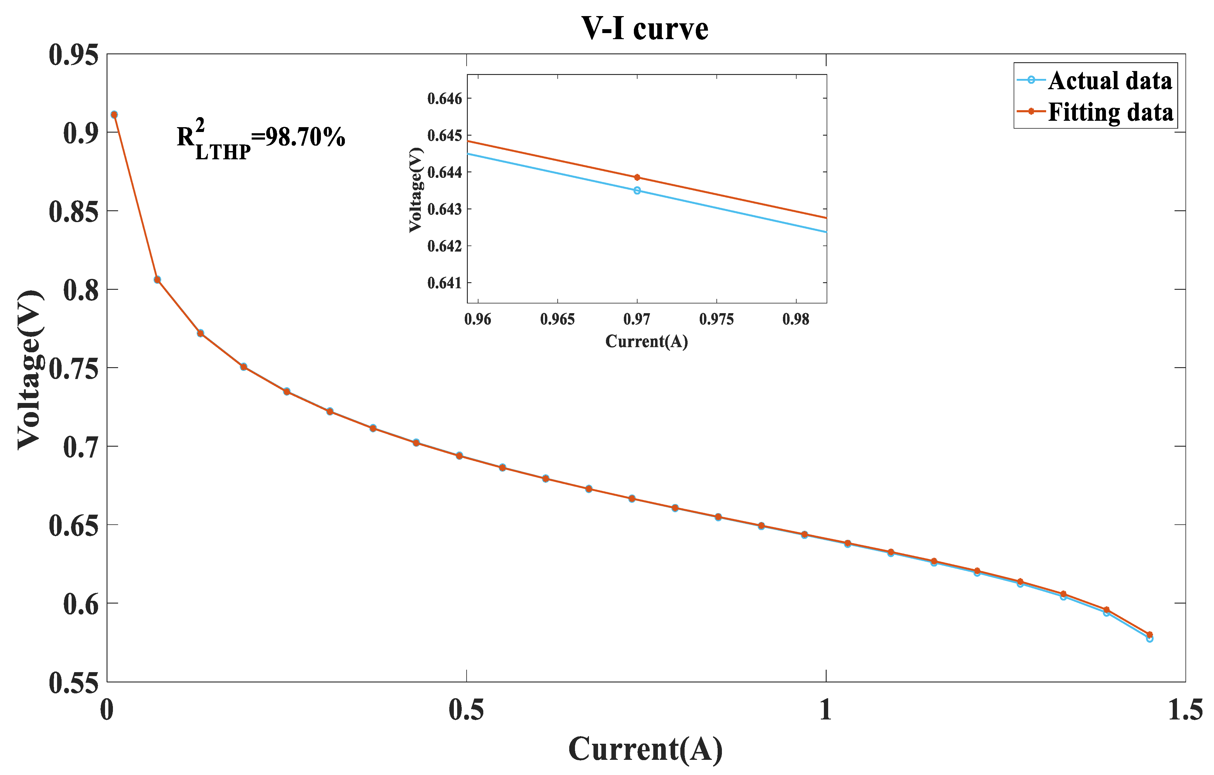
Figure 22 shows the V-I characteristic curves based on low-temperature and high-pressure obtained by GRNN fitting the MFO algorithm under noise reduction data cases. It can be obtained by observation that the curve of fitting data almost coincides with the curve of actual data and the error measured by RMSE is equal to 98.70%, which demonstrates the parameter identification effect is in line with expectations.

4.4.2. Insufficient Data

Table A6. Parameters identification results of original data and predicted data based under LTHP and MhAs.

State	Algorithms	Data	Identified Parameters							RMSE
			ԑ1	ԑ2	ԑ3	ԑ4	λ	Rc(Ω)	b(V)
LTHP	MPA	O	−0.9778	3.5659 × 10−3	9.7853 × 10−5	−1.7098 × 10−4	16.4825	8.0000 × 10−4	0.0169	3.9481 × 10−5
		P	−0.9494	3.4339 × 10−3	9.4921 × 10−5	−1.7101 × 10−4	17.0471	7.9376 × 10−4	0.0170	1.2754 × 10−5
	AEO	O	−0.9935	3.1003 × 10−3	6.1264 × 10−5	−1.7103 × 10−4	15.4458	5.4652 × 10−4	0.0167	3.9974 × 10−5
		P	−0.9575	3.0169 × 10−3	6.3508 × 10−5	−1.7106 × 10−4	16.0734	4.7360 × 10−4	0.0169	1.3427 × 10−5
	PSO	O	−0.9703	2.9028 × 10−3	5.0162 × 10−5	−1.6158 × 10−4	15.0542	2.0792 × 10−4	0.0328	3.4588 × 10−2
		P	−0.9990	2.7318 × 10−3	3.6000 × 10−5	−1.4170 × 10−4	10.1816	5.8666 × 10−4	0.0420	1.9711 × 10−2
	BAS	O	−0.9182	3.0406 × 10−3	7.5044 × 10−5	−1.7750 × 10−4	13.8505	4.2091 × 10−4	0.0301	3.1607 × 10−2
		P	−0.9931	3.1320 × 10−3	5.9052 × 10−5	−1.7616 × 10−4	15.8719	3.5783 × 10−4	0.0192	6.0350 × 10−3
	GWO	O	−1.1501	3.6883 × 10−3	6.7517 × 10−5	−1.7042 × 10−4	10.4514	2.1721 × 10−4	0.0146	3.6019 × 10−4
		P	−1.0010	3.0434 × 10−3	5.5508 × 10−5	−1.7142 × 10−4	17.3989	4.1713 × 10−4	0.0172	1.0451 × 10−4
	MFO	O	−0.9458	3.0558 × 10−3	6.8896 × 10−5	−1.7060 × 10−4	10.0000	8.0000 × 10−4	0.0136	5.6641 × 10−4
		P	−0.9375	2.5788 × 10−3	3.6958 × 10−5	−1.7101 × 10−4	16.5422	8.0000 × 10−4	0.0169	4.1393 × 10−5

of Appendix A shows the statistics of the results of parameter extraction of insufficient and predicted data, respectively, by six algorithms under LTHP. From Table A6 of Appendix A, it is obvious that after data prediction, the RMSE obtained by the six algorithms is lower than that obtained from predicted data. After data prediction, the RMSE of the PSO algorithm and the BAS algorithm has a magnitude not exceeding the minus third power of ten, while the RMSE of the other algorithm has a magnitude exceeding the minus fourth power of ten. The MFO algorithm exhibits the most significant decrease of 92.69%, whereas the PSO algorithm demonstrates a comparatively smaller reduction of 43.01%.

Figure 23 describes the RMSE convergence curves obtained by six algorithms on two datasets, with all algorithms having lower RMSE based on predicted data.

The boxplot illustrates the distribution of RMSE obtained by MhAs which is presented in Figure 24. It can be obtained by observation that except for the BAS and PSO, the RMSE of other algorithms obtained from predicted data has decreased. However, the lower bound RMSE of PSO and the upper bound RMSE of BAS have increased. In addition, MPA, AEO, and MFO have superior performance compared with other algorithms. This fully shows that GRNN data noise reduction can improve the stability of MhAs in parameter identification.

5. Discussions

Table 2. Summary of research on parameter identification of some PEMFCs in recent years.

Approach	Year	Cell Type	Data Process			Operating Condition
			Data De-Noise	Data Prediction	No	Consider	No Consider
BRNN-MhAs [17]	2021	Ballard-Mark-V PEMFC	✓			✓
IDE [14]	2021	N.P.	✓				✓
LMBP [15]	2021	Ballard-Mark-V PEMFC			✓	✓
ICSO [13]	2023	N.P.			✓	✓
ELM-MhAs [12]	2023	Ballard-Mark-V PEMFC	✓			✓

Note. N.P.: Not provided.

summarizes the research related to PEMFC parameter identification in recent years. It can be seen from the statistical comparison results that most studies have not simultaneously considered the impact of noise data and insufficient data volume on the final parameter extraction accuracy. The research conducted in this study precisely compensates for the shortcomings in this area and provides excellent guidance for the research on PEMFC parameter extraction direction. However, through the research in this study, it can be found that in using heuristic algorithms, due to their unique parameter random search ability, some algorithms have abnormal numerical accuracy in the results when extracting parameters. For example, under MTMP conditions, after data prediction and parameter extraction using the BAS algorithm, the identification accuracy showed abnormalities, after data de-noising, and the accuracy decreased by 13.26%. Overall, the method proposed in this research is not only suitable for PEMFC parameter identification but also for photovoltaic (PV) and solid oxide fuel cell (SOFC) parameter identification. Through this study, it has been fully demonstrated that it has extremely good performance in the field of parameter identification. All experimental results in this article are based on the data in

Table A7. Original data under HTLP condition [39].

V	I
0.0100	0.9817
0.0700	0.8619
0.1300	0.8233
0.1900	0.7993
0.2500	0.7817
0.3100	0.7677
0.3700	0.7560
0.4300	0.7459
0.4900	0.7370
0.5500	0.7289
0.6100	0.7215
0.6700	0.7147
0.7300	0.7082
0.7900	0.7021
0.8500	0.6963
0.9100	0.6906
0.9700	0.6850
1.0300	0.6795
1.0900	0.6740
1.1500	0.6684
1.2100	0.6625
1.2700	0.6562
1.3300	0.6491
1.3900	0.6404
1.4500	0.6272

,

Table A8. Original data under MTMP condition [39].

V	I
0.0100	0.9439
0.0700	0.8314
0.1300	0.7950
0.1900	0.7723
0.2500	0.7556
0.3100	0.7422
0.3700	0.7310
0.4300	0.7213
0.4900	0.7126
0.5500	0.7047
0.6100	0.6975
0.6700	0.6907
0.7300	0.6843
0.7900	0.6782
0.8500	0.6723
0.9100	0.6665
0.9700	0.6608
1.0300	0.6551
1.0900	0.6493
1.1500	0.6434
1.2100	0.6371
1.2700	0.6302
1.3300	0.6223
1.3900	0.6124
1.4500	0.5969

and

Table A9. Original data under LTHP condition [39].

V	I
0.0100	0.9112
0.0700	0.8061
0.1300	0.7720
0.1900	0.7506
0.2500	0.7349
0.3100	0.7222
0.3700	0.7115
0.4300	0.7023
0.4900	0.6940
0.5500	0.6864
0.6100	0.6794
0.6700	0.6728
0.7300	0.6666
0.7900	0.6606
0.8500	0.6548
0.9100	0.6491
0.9700	0.6435
1.0300	0.6378
1.0900	0.6320
1.1500	0.6259
1.2100	0.6195
1.2700	0.6125
1.3300	0.6043
1.3900	0.5940
1.4500	0.5777

, where Table A7 represents the V-I data of PEMFC under HTLP, Table A8 represents the V-I data under MTMP, and Table A9 represents the V-I data under LTHP.

Additionally, the study did not take into account the impact of changes in temperature and other factors on the identification results during the actual operation of the PEMFC, and the shortcomings of this study are that although the overall accuracy can be improved after data processing, it has not improved much. Further research is needed in this direction in the future. Additionally, the research did not consider the specific impact and role of the identified parameters on the cell itself [36,37,38].

6. Conclusions and Prospect

This study proposes a parameter identification method for the PEMFC using GRNN and MhAs. The original cell V-I data are processed using GRNN, which includes data de-noising and data prediction. In addition, six typical heuristic algorithms were used to extract parameters of the PEMFC under three operating conditions: HTLP, MTMP, and LTHP. Then, the obtained results were compared with the results extracted from the original data, and the results show that using GRNN to process the data can markedly enhance the precision rate of final identification, specifically, after data prediction, the accuracy of the MFO algorithm has been improved by 92.69% under LTHP conditions. And after data de-noising processing, it is obvious that it can improve the stability of parameter identification results. Finally, by substituting the identified parameters into the model, the fitting accuracy of V-I data obtained under all three operating conditions was very high. Specifically, under HTLP conditions, the V-I fitting accuracy achieved 99.39%, the fitting accuracy was 99.07% on MTMP, and the fitting accuracy was 98.70%. All in all, after processing the PEMFC data using GRNN and using MhAs for cell parameter extraction, the efficiency, accuracy, and stability of the final identification results of PEMFC parameter identification can be greatly improved. This study provides a novel approach to the field of PEMFC parameter identification.

In the end, this study provides significant guidance for future research on PEMFC parameter extraction. However, future research on this aspect should pay more attention to the impact of data analysis on the final identification results. In addition, consideration should also be given to the impact of the identified parameters on the internal mechanism of the cell itself. In general, further research should be conducted on the internal characteristics of the cell, such as its state of charge and health, through the identified parameters.