Abstract
The aim of this paper is to present a methodology for the calculation of the R-L parameters of a model of a nonlinear hysteretic inductor. The methodology is based on the analysis of the instantaneous magnetising power calculated from the hysteresis loop of the inductor and is completely developed in the time domain. The instantaneous magnetising power is firstly separated into the oscillatory and absorbed components. Thereafter, the parameter R is calculated using the absorbed component and the parameter L using the oscillatory component. The methodology is validated through the comparison of the results for parameters R and L obtained with the proposed method and the existing method based on the Poynting theorem. The validation is demonstrated on the specific simulated cases with idealised parameters of a nonlinear circuit. Additionally, the paper presents results for the parameters R and L calculated from the hysteresis loops measured at frequencies from 1 to 300 Hz. Furthermore, the fitting functions representing the variation of these parameters with the rate of change of magnetic flux density, and the corresponding results, are presented in the paper. A discussion of all the results presented and applicability of the methodology proposed, as well as the concluding remarks, are given thereafter.
1. Introduction
A description of the behaviour of nonlinear electric circuits with magnetic cores employed in electric machines during steady-state and transient working regimes usually requires knowledge of the magnetic characteristics of the material used (magnetisation curve, i.e., the (magnetic flux vs. current) dependence, hysteresis loops, power losses, etc.) [1,2,3,4,5,6,7,8]. Such an electric circuit can alternatively be represented by: (1) an inductance L exhibiting a single-valued (SV, thus neglecting hysteresis) magnetisation curve connected in parallel to a resistance R [1], (2) a dynamic hysteretic core model [1] or (3) an electric network (such as a Cauer circuit [3,4]).
The first and the third options are suitable for the incorporation of nonlinear magnetic cores or electric machine models into a complex electric circuit, which may include power electronics, load, and other electric components of interest. In many cases, for the purpose of simplification, the inductance L (with SV characteristic) is considered as static (not dynamic), which leads to errors in calculations and improper representation of the behaviour of nonlinear magnetic cores [9]. The second option is often required by the power engineers and designers of electrical equipment for power systems. They need an accurate dynamic model for the proper representation of specific transients in the electrical network during faults, ferroresonance events in the power transformer, influence of geomagnetically induced currents on the power transformer or parallel operation of DC and AC systems [10,11].
The simulation of circuits containing ferromagnetic cores may be focused on the implementation of an appropriate hysteresis model. There are several useful descriptions readily used in electrical engineering, such as the bottom-up Preisach model [12,13] or the top-down formalism developed by Jiles and Atherton [14]. In the present paper, we focus instead on an alternative, circuit-based description, which sheds some light on energy-related issues, without a discussion of the caveats and limitations of the hysteresis models used. Readers more interested in hysteresis modelling are referred to an excellent review paper published recently [10].
Representation of the parallel inductance and resistance branches (the R-L model) is probably the simplest way to describe nonlinear magnetic circuits. However, such a description needs to have a clear physical meaning when it comes to “describing the transfer of power and energy between a source and a load”, as pointed out in [15].
The identification of instantaneous active and reactive power from terminal measurement of electric voltage and current allows identification of R and L parameters in different configurations of linear or nonlinear series and parallel R-L circuits [15]. Geometric algebra (GA) and differential geometry concepts were also used for the calculation of instantaneous powers and circuit parameters (R, L and C) from the terminal measurement of voltage and current [16].
A methodology based on harmonic analysis was also used for the calculation of the instantaneous magnetising power, and the absorbed and oscillatory components, of a toroidal core made of electrical steel [17]. After measurement of the hysteresis loop of the core, the harmonics of the magnetic field were calculated and used for determination of its two components, related to the absorbed and the oscillatory power. This allowed the subsequent calculation of the R and L parameters of such a nonlinear inductor without prior modelling of the magnetic hysteresis. The methodology for this calculation was demonstrated in the paper. Both parameters, i.e., R and L, were expressed in the time domain as time-varying quantities. Furthermore, their dependence on the rate of change of the magnetic flux density B was examined, as well as the possibility of representing such dependence with a suitable function.
The rest of the paper is structured as follows. Firstly, the paper presents the results needed for the validation of the methodology, i.e., simulated piecewise hysteresis loop and magnetisation curve and experimental hysteresis loops, measured for a toroidal core made of grain-oriented electrical steel at 0.5, 1.0 and 1.5 T of maximum magnetic flux density, for frequencies of 1, 50, 100, 200 and 300 Hz. Consequently, the validation is demonstrated through the comparison of some of the results for R and L obtained by the proposed methodology to those obtained with an existing method. After validation, the paper gives the results of the calculation of parameters R and L in the time domain obtained using all the experimental results. Subsequently, the dependencies of R and L values on the rate of magnetic flux density dB/dt are discussed and suitable functional dependencies for their trends are provided. Finally, observations from the study and an analysis for an example of an application of the considered methodology applied to solving a simple electric circuit with a nonlinear hysteretic inductor are discussed.
2. R-L Model of Nonlinear Hysteretic Inductor
A nonlinear hysteretic inductor Lh(t), which contains a ferromagnetic core, can be simply represented with a parallel connection of a nonlinear non-hysteretic inductor L(t) and nonlinear resistor R(t), as shown in Figure 1 [18]. Such representations are well-known in the literature and thus will be just briefly discussed in this paper.
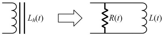
Figure 1.
Equivalent electric circuit of a nonlinear hysteretic inductor.
The resistance R(t) is usually calculated as a ratio of the voltage across the resistor and its current. It has been shown that the current of this resistance is a hysteretic current iH(t), a component of the total current i(t) of the inductor Lh(t), whereas the voltage can be calculated as a time derivative of the magnetic flux ϕ(t) in Lh(t) [15]. The remaining current, named saturating current iS(t), flows through the inductor L(t). Its inductance can be calculated as a derivative of ϕ(t) with respect to iS(t) [15]. Accordingly, the following equations can be written:
where .
This approach has been tested on a number of electric circuits with an inductor Lh and additional series or parallel resistors and inductors (linear or nonlinear ones). The identification of the circuit parameters allows the calculation of instantaneous active and reactive power in the circuit according to the terminal voltage and current measurement [15]. The obtained results of the simulations confirm the applicability of the approach to the analysis of circuits with a nonlinear hysteretic inductor. The hysteresis loop (or loops) of the hysteretic inductor should be known in advance. This approach complies with the Poynting theorem and explains the physical meaning of the instantaneous powers and circuit parameters.
Another methodology based on GA has been also developed recently for the calculation of electric circuit parameters based on the terminal voltage and current measurement [16]. The methodology has also been found to be suitable for implementation in circuits which, besides resistors and inductors, also include capacitors. Cases with nonlinear components, including resistor and switch connections and nonlinear (but not hysteretic) inductors, have been analysed. Instantaneous powers in the circuit are determined upon the identification of circuit parameters, as shown in Figure 2.
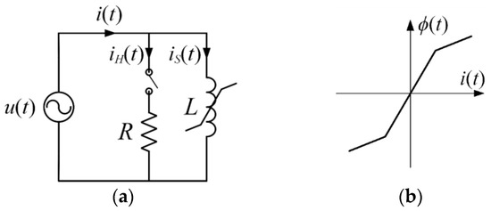
Figure 2.
(a) Electric circuit with resistor and switch series connection and parallel nonlinear inductor; (b) piecewise magnetising curve.
The instantaneous power of a hysteretic inductor has also been recognised as an important subject in a number of recent research papers [5,6,17,19,20,21]. Bramerdorfer et al. carried out a comprehensive review of state-of-the-art methods for the characterisation of soft magnetic materials used in the magnetic circuits of electric machines [5]. The evolution of approaches in both the time and frequency domain were discussed. Corti et al. focused on the issue of how to estimate the core losses of an inductor operating in an electronics power engineering device (a DC-DC buck converter) in a reliable manner. The authors indicated the advantages of analysis in the time domain in which the non-uniformity of the field was taken into account [6].
In [17], harmonic analysis was applied to the separation of the instantaneous magnetising power per unit volume p(t) to its components—absorbed pa(t) (equivalent to active power in [15]) and oscillatory po(t) power (equivalent to reactive power in [15]). These two powers are defined with the following expressions:
where H(t) = HS(t) + HC(t), HS(t) and HC(t) are magnetic field strength components, representing hysteretic (sine) and saturation (cosine) properties, respectively, whereas B(t) is the flux density of the measured hysteresis loop. The corresponding waveforms are presented in Figure 3.
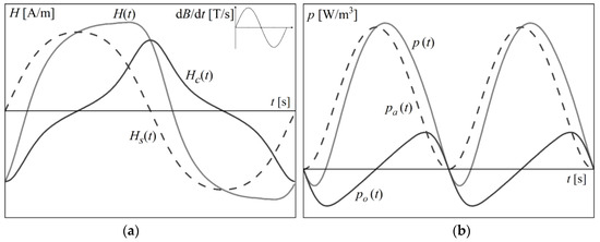
Figure 3.
Waveforms of: (a) H(t), HS(t) and HC(t); and (b) p(t), pa(t) and po(t), for sinusoidal B(t).
Based on this methodology, a more general definition of the nonlinear parameters R and L of the nonlinear hysteretic inductor Lh can be derived as follows:
where is the voltage at the inductor coil, is the cosine (saturating) component of the current, l and S are the mean magnetic path length and cross-sectional area of the inductor core, V = Sl is the core volume and N is the number of turns in the coil of inductor Lh.
3. Simulated and Experimental Data for Validation
To validate the proposed methodology, a number of comparisons between the results obtained using the methodology proposed and other methodologies were performed. These comparisons were made for some of the simulated cases considered by other methodologies and for new experimental data.
The first simulated case (Case I) originally considered a series connection of the linear resistor and the hysteretic inductor with a piecewise linear loop. As the methodology proposed considers only the hysteretic inductor (without additional series or parallel components), the resistance of the linear resistor was set to zero. Furthermore, a different scale was used for the piecewise loop, considering a B(H) loop instead of a ϕ(i) loop (ϕ is the magnetic flux and i is the electric current of the inductor) used in the original example [15]. The simulated loop is presented in Figure 4.
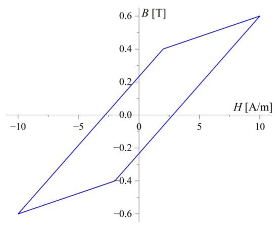
Figure 4.
Simulated piecewise hysteresis loop.
The second simulated case (Case II) originally considered the electric circuit in Figure 2 for several combinations of switch position and inductor operation regime [16]. The model with a closed switch and saturated inductor was considered for comparison. However, the same methodology based on (1) and (2) was used again instead of the original methodology based on GA. The reasons are the significant differences in the implementation of the GA-based methodology and other two methodologies, and the current non-consideration of hysteresis in the GA-based methodology.
Other comparisons were also made with hysteresis loops measured for a toroidal core made of grain-oriented electrical steel sheet (grade 27PH100, produced by POSCO [22]). The loops were measured using a standard method for characterisation of toroidal cores, with a PC-based experimental setup as described in detail in [23]. Measurements were performed under controlled sinusoidal shape of the induced voltage (flux density B) for Bmax equal to 0.5, 1.0 and 1.5 T at frequencies f equal to 1, 50, 100, 200 and 300 Hz. The obtained loops are presented in Figure 5. A comparison of the results obtained using Equations (1), (2), (5) and (6) was performed using these results.
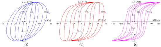
Figure 5.
Measured hysteresis loops at: (a) 0.5 T; (b) 1.0 T; (c) 1.5 T, for 1 to 300 Hz.
4. Methodology Validation—Comparisons of Results
A code was written in Wolfram Mathematica software (version 13) which implements both methodologies and returns the results for R and L parameters for the considered case. A comparison of the calculated L obtained for Case I is presented in Figure 6, whereas Figure 7 shows a comparison of calculated R and L obtained for Case II. For brevity, only one half of the period is presented due to the symmetry in the results obtained in the second half.
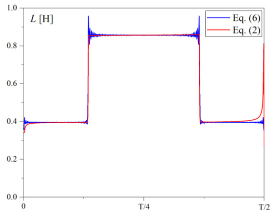
Figure 6.
Comparison of the results for L for Case I.
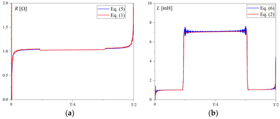
Figure 7.
Comparison of the results for: (a) R; and (b) L, for Case II.
From comparisons of the computation results obtained with both methods, it follows that a good agreement was obtained, and that both methods are basically equivalent. The results for Case I agree shape-wise with the original results given in [15], but in a different scale, whereas the results for Case II agree both in the shape and in values, as the original results given in [16] show that the resistance amounts for 1 Ω and the inductance switches between 1 mH and 7 mH. The results oscillate at the beginning and the end of the time period because of the zero crossings of the corresponding quantities in (1) and (2) and (5) and (6). Additionally, the results obtained using (6) oscillate when a fast transition occurs, due to the time derivative of iC(t) and the Gibbs phenomenon due to Fourier transformation [24,25].
Other comparisons were performed with experimental results, using waveforms of H and B for hysteresis loops from Figure 5. The obtained results are presented in Figure 8, and for brevity the data for 200 and 300 Hz are not shown as they show similar qualitative performance.
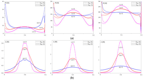
Figure 8.
Comparison of the results for: (a) R; and (b) L, obtained with experimental results for 1, 50 and 100 Hz (from left to right).
The results for the two methods are in good agreement, except for R vs. time dependence at the beginning and at the end of the considered time intervals (half-periods). The results obtained using (5) deviate less and show a tendency towards a relatively stable value at the beginning and the end, whereas the results obtained using (1) are more numerically unstable and diverge at the discontinuity (at zero crossing). The difference between (1) and (5) is in the waveforms of the quantities; the ones in (1) periodically change from positive to negative half-periods (containing relatively fast zero crossing), whereas the ones in (5) are positive during the whole period. Such deviation does not exist in the results for the inductance L as corresponding quantities in (2) and (6) are in phase at the zero crossing.
5. Results for R and L and Analysis of R = g(B′/f) and L = h(B′/f) Dependencies
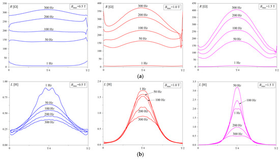
All results for the parameters R and L obtained using the experimental results given in Figure 5 are presented in Figure 9. Results have been grouped by Bmax for better observation of their variation with the frequency.
Representation of the inductor Lh with the equivalent parameters R and L allows its consideration within electric circuits of practical interest. As can be seen from Figure 8, the parameters R and L vary with the time during the illustrated half-period of the magnetisation cycle (with an identical change in the second half-period). This time variation makes the practical application of the results for R and L more complex, and requires usage of iterative or numerical solving methods, but the final solutions of electric circuits containing an inductor Lh would be more accurate and give better physical representation of the electric power flow in comparison to the solution with constant values of R and L. For easier practical implementation and solving of the electric circuit with such an inductor, it would be better to consider the variation of R and L with some electric quantity, such as the electric current or voltage. As shown in Figure 1, R and L are connected in parallel and they have the same voltage at their ends. The quantity equivalent with this voltage is the rate of change of magnetic flux density, namely B′ = dB/dt. Since B′ is different for each f, at particular Bmax, a normalised quantity B′/f, which does not change with f, was used as the independent variable in the curve fittings. Thus, the dependencies R = g(B′/f) and L = h(B′/f) for some cases from Figure 9 are presented in Figure 10. Along with the experimental results, the fits of the functions f and g are given in Figure 10. Experimental data for R = g(B′/f) and L = h(B′/f) were fitted to the exponential functions in the form:
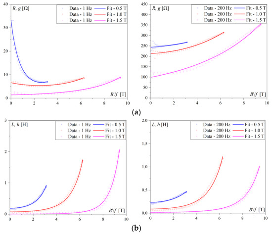
Figure 10.
Part of results for: (a) R = g(B′/f); and (b) L = h(B′/f); dependencies at 1 and 200 Hz.
This form of equations was chosen arbitrarily, but, as evident from Figure 10, it gives good approximation of the data. Other sigmoidal or polynomial functions can also be used.
The results presented in Figure 10 show clearly that parameters R and L can be well fitted to a function dependent on B′/f. Similarly, good fittings were also obtained from other results presented in Figure 9. The fitting results are summarised in Figure 11. Values of the fitting parameters a, b, c, l, m, and n (of Equation (7)) for all considered cases are given in Table 1.
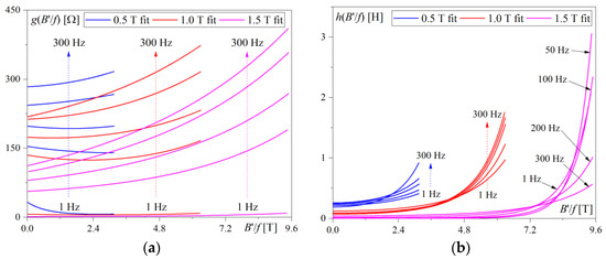
Figure 11.
Results for fitting functions: (a) g; and (b) h, obtained with experimental results given in Figure 5.

Table 1.
Values of the fitting parameters a, b, c, l, m and n in Equation (7).
6. Discussion of Results and Application of Methodology
The results for resistance R and function g(B′/f) presented in Figure 9 and Figure 11 clearly show their increase with frequency. As can be seen in the inset in Figure 3, the magnetic flux density B starts from its minimum; thus, B′ starts from the zero and increases to the maximum at T/4. The waveform of the absorbed power pa exhibits a similar behaviour. The resistance at 1 Hz for all Bmax values and at 50 Hz and 100 Hz at 0.5 T can be considered as constant when compared to all other cases. However, at higher f and Bmax, the resistance varies between the minimal and a maximal value, reaching a minimum when B′ is equal to zero (B reaches minimum/maximum) and maximum when B′ is at maximum/minimum (B is equal to zero).
In contrast to R, the inductance L and function h(B′/f) decrease with the increase of the frequency, except for two cases at 1.5 T and 50 Hz and 100 Hz, as can be seen in Figure 9 and Figure 11. The parameter L also varies from the minimum to the maximum value with the change of B′, in a similar way as the parameter R does, but with a more pronounced difference between the two extreme values. The minimal value of L stays practically constant for all frequencies at a particular Bmax, and it decreases with the increase of Bmax, reaching almost zero for 1.5 T. The last observation corresponds to the fact that the permeability of the ferromagnetic material tends to the permeability of vacuum at the tip of the major hysteresis loop (or close to the saturation).
The behaviour of both parameters, i.e., R and L, or more precisely its variation in time, is very complex. It is not easy to find simple regularity in the waveforms (Figure 9), in the fits (Figure 11) or in the fitting parameters (Table 1). Finding some regularities could be expected in future research on this issue, under certain conditions and for more focused studies than this one. One of the problems is that all the losses are lumped together in a single parameter of R, but in reality there are various components of this loss, attributed for instance to hysteresis and eddy currents. However, such separation of loss components in the time domain is much more complex and was not attempted in this study.
Thus, in the next section of this paper, we focus on the application of the methodology and the obtained results. For that purpose, a simple electric circuit with series connection of an additional resistor Ra and nonlinear hysteretic inductor Lh and AC voltage source was considered, as presented in Figure 12. Inductor Lh is represented with its equivalent parameters R and L. The resistance Ra amounted to 48 Ω, the input voltage u(t) amplitudes were 12 V and 16 V and the frequency was 100 Hz.
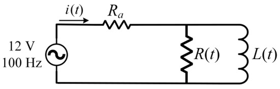
Figure 12.
Electric circuit with additional resistor Ra and equivalent R and L parameters of a nonlinear hysteretic inductor Lh.
Such a problem requires finding a unique value of the unknown electric current i(t) in the circuit in Figure 12. However, the values of R and L are also unknown, and they need to be determined during the solution procedure. By applying the basic laws to the circuit in Figure 12, the following relations are obtained:
where is the voltage at the terminals of R and L, and and are the currents in the branches with R and L, respectively.
The solution of (8)–(10) was obtained iteratively. In the first step, all currents were set to zero (, and ). Then, was calculated from (8) and dB(t)/dt from (9) (as well as the corresponding Bmax). According to the obtained Bmax, all fitting parameters were calculated by applying a linear interpolation to a set of data given in Table 1. The parameters R and L were calculated using (7) after insertion of the obtained fitting parameters and dB(t)/dt. After this step, a new iteration was started with a calculation of new estimates of and using (9), as well as using (10). Thereafter, all other calculations were repeated until the convergence of the solution for i(t) was obtained (when the difference between two consecutive waveforms of i(t) was lower than the set limit, such as 0.5%). Typical convergence was 12 to 15 iterations.
The solutions were obtained for two amplitudes of input voltage u(t), equal to 12 and 16 V, at the frequency of 100 Hz. The results of the calculation are presented in Figure 13, along with the experimental results obtained in the real circuit from Figure 12. A comparison of calculated and measured results shows good agreement in the waveforms’ shape and phase, whereas a difference in amplitudes exists around 9.7% at 12 V and around 8.3% at 16 V of input voltage. Such difference in the amplitude is a consequence of a low number of input data (three sets only, obtained for 0.5, 1.0 and 1.5 T) and linear interpolation applied to these data (even though the data have nonlinear dependence on Bmax). For better accuracy, input data should consist of at least ten sets and some higher-order interpolation should be applied. Even so, the results in Figure 13 confirm the applicability of the methodology presented in solving of simple dynamic electric circuits. Its applicability to the complex circuits needs to be further tested, which is beyond the scope of the present work.
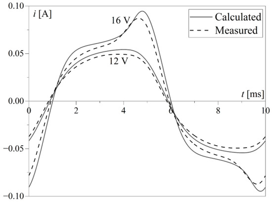
Figure 13.
Comparisons of calculated and measured electric current i(t).
Furthermore, it is reasonable to assume that the results for the parameters R and L obtained using the presented methodology can be used as the input data for training neural networks or for improved fitting using some metaheuristic algorithms. Such solutions could be the basis for computer software for solving the dynamic electric circuits with a complex configuration and a higher number of linear and nonlinear/hysteretic components.
7. Conclusions
This paper presents a methodology for calculation of the equivalent parameters R and L of a nonlinear hysteretic inductor Lh. The methodology firstly considers the magnetising power p(t) of the inductor Lh, which is physically consistent with Poynting’s theorem, and its two components, the absorbed power pa(t) and the oscillatory power po(t). Secondly, a more general (physically based) expressions for parameters R and L, based on these two power components, were proposed. The form of expression for R is known in the theory of linear circuits for linear resistors. However, it has been rarely used (or may even have been used for the first time) for the calculation of the parameter R variable with time, which increases its importance. Expression of L, which varies with time, was not found by the authors in the existing literature. It gives the same result as the expression based on the magnetic flux, but it also complements the expression for R and it has a more physically sound form, which can be easily interpreted in terms of Poynting’s theorem. This gives it additional importance in comparison to the existing methodologies.
The presented methodology was validated on a number of examples, using simulated and experimental results, through comparisons with another methodology. Upon a successful validation, special attention was paid to the experimental results and calculation of real R and L parameters for a toroidal core made of grain-oriented electrical steel. These parameters were calculated for one quasi-static case (at a frequency of 1 Hz) and four dynamic cases (at frequencies of 50, 100, 200 and 300 Hz), at corresponding amplitudes of the magnetic flux density equal to 0.5, 1.0 and 1.5 T. To the authors’ knowledge, this is the first time that such a large number of cases has been considered when the time-varying parameters R and L are calculated.
Furthermore, it was shown that the parameters R and L can be easily related to the rate of change of the magnetic flux density (B′), which is directly proportional to the electric voltage at the ends of the inductor Lh. In this paper, such relation was considered by fitting the calculation data for R and L to a relatively simple exponential function with B′ as an independent variable. It was found that their relation is complex under dynamic conditions. Such results could be useful for a more comprehensive insight into the behaviour of R and L under dynamic conditions, or when the material is exposed to variable mechanical or temperature conditions.
As a proof of its practical importance, the presented methodology was applied to solve a simple electric circuit containing a nonlinear hysteretic inductor. A solution of the unknown electric current in the circuit was obtained through an iterative procedure. The calculated waveforms of the current for two considered amplitudes of the input voltage were compared to the measured waveforms of the real circuit. Very good agreement between the shapes and phases of the waveforms was obtained, and the amplitudes differed by less than 10%, which was found to be acceptable for the limited set of input parameters and the purposely simplified interpolation applied.
The presented methodology can serve as a foundation for further investigation of the equivalent parameters of nonlinear and hysteretic electric circuit components. It can be further developed by considering more specific characteristics of ferromagnetic materials, such as anisotropy, domain structure and similar characteristics. It should be tested on more complex electric circuits with nonlinear hysteretic inductors to prove its practical importance. Finally, it could be incorporated into existing or new computer programs (solvers) of electric circuits with nonlinear and hysteretic components so that much simpler SPICE analogues could be extracted from the system behaviour.
Future research on this subject will be devoted to the application of the methodology presented in the analysis of more complex devices, such as power transformers, electrical machines or variable inductors. Determination of their circuit parameters in the proposed manner would be useful in more precise analyses of their behaviour under various working regimes or energy efficiency and power factor calculation. However, deeper treatment regarding specific devices is beyond the scope of this paper.
Author Contributions
Conceptualisation, S.D., M.R. and B.K.; methodology, B.K.; software, S.D. and M.R.; validation, S.Z., K.C. and M.V.; formal analysis, M.V.; investigation, S.D. and B.K.; resources, B.K.; data curation, S.D. and M.R.; writing—original draft preparation, S.D. and B.K.; writing—review and editing, S.Z. and K.C.; visualisation, S.D., M.R. and B.K; supervision, B.K.; project administration, M.R.; funding acquisition, M.R., B.K. and K.C. All authors have read and agreed to the published version of the manuscript.
Funding
B.K., M.R. and K.C. are grateful for financial support within the framework of the Program No. 020/RID/2018/19 “Regional Initiative of Excellence” granted by the Polish Minister of Science and High Education in the years 2019–2023, from which the costs of mutual visits of these scientists to Częstochowa/Čačak, respectively, were covered, leading to fruitful discussions which stimulated the joint cooperation. This study was supported by the Ministry of Science, Technological Development and Innovation of the Republic of Serbia, and these results are parts of the Grant No. 451-03-47/2023-01/200132 with University of Kragujevac—Faculty of Technical Sciences Čačak.
Data Availability Statement
Data available from the corresponding author upon request.
Conflicts of Interest
The authors declare no conflict of interest.
References
- Rezaei-Zare, A.; Iravani, R. On the Transformer Core Dynamic Behavior During Electromagnetic Transients. IEEE Trans. Power Deliv. 2010, 25, 1606–1619. [Google Scholar] [CrossRef]
- Hane, Y. Hysteresis Modeling for Power Magnetic Devices Based on Magnetic Circuit Method. J. Magn. Soc. Jap. 2022, 46, 22–36. [Google Scholar] [CrossRef]
- Suehiro, I.; Mifune, T.; Matsuo, T.; Kitao, J.; Komatsu, T.; Nakano, M. Ladder Circuit Modeling of Dynamic Hysteretic Property Representing Excess Eddy-Current Loss. IEEE Trans. Magn. 2018, 54, 7300704. [Google Scholar] [CrossRef]
- Minowa, N.; Takahashi, Y.; Fujiwara, K. Iron Loss Analysis of Interior Permanent Magnet Synchronous Motors Using Dynamic Hysteresis Model Represented by Cauer Circuit. IEEE Trans. Magn. 2019, 55, 7401404. [Google Scholar] [CrossRef]
- Bramerdorfer, G.; Kitzberger, M.; Wöckinger, D.; Koprivica, B.; Zurek, S. State-of-the-art and Future Trends in Soft Magnetic Materials Characterization with Focus on Electric Machine Design—Part 2. TM Tech. Mess. 2019, 86, 553–565. [Google Scholar] [CrossRef]
- Corti, F.; Reatti, A.; Lozito, G.M.; Cardelli, E.; Laudani, A. Influence of Non-Linearity in Losses Estimation of Magnetic Components for DC-DC Converters. Energies 2021, 14, 6498. [Google Scholar] [CrossRef]
- Chwastek, K.R. The Effects of Sheet Thickness and Excitation Frequency on Hysteresis Loops of Non-Oriented Electrical Steel. Sensors 2022, 22, 7873. [Google Scholar] [CrossRef]
- Zhao, X.; Yang, L.; Xu, H.; Huang, K.; Liu, L.; Du, Z. Dynamic Hysteresis and Loss Modeling of Grain-Oriented Silicon Steel Under High-Frequency Sinusoidal Excitation. IEEE Trans. Magn. 2022, 58, 7300805. [Google Scholar] [CrossRef]
- Štumberger, G.; Plantić, Ž.; Štumberger, B.; Marčič, T. Impact of Static and Dynamic Inductance on Calculated Time Responses. Przegl. Elektrotechn. 2011, 87, 190–193. [Google Scholar]
- Mörée, G.; Leijon, M. Review of Hysteresis Models for Magnetic Materials. Energies 2023, 16, 3908. [Google Scholar] [CrossRef]
- Sun, Y.; Zhang, L.; Zhang, Z.; Wang, D. Overview of Research Status of DC Bias and Its Suppression in Power Transformers. Energies 2022, 15, 8842. [Google Scholar] [CrossRef]
- Preisach, F. Űber die magnetische Nachwirkung (On the magnetic aftereffect—in German). Z. Phys. 1935, 94, 277–305. Available online: https://ieeexplore.ieee.org/abstract/document/7857913 (accessed on 23 June 2023). [CrossRef]
- Mayergoyz, I.D. Mathematical Models of Hysteresis and Their Applications, 2nd ed.; Elsevier: Amsterdam, The Netherlands, 2003. [Google Scholar]
- Jiles, D.C. Atherton D.L. Theory of ferromagnetic hysteresis. J. Magn. Magn. Mater. 1986, 61, 48–60. [Google Scholar] [CrossRef]
- de León, F.; Qaseer, L.; Cohen, J. AC Power Theory from Poynting Theorem: Identification of the Power Components of Magnetic Saturating and Hysteretic Circuits. IEEE Trans. Power Deliv. 2012, 27, 1548–1556. [Google Scholar] [CrossRef]
- Montoya, F.G.; de León, F.; Arrabal-Campos, F.; Alcayde, A. Determination of Instantaneous Powers from a Novel Time-Domain Parameter Identification Method of Non-Linear Single-Phase Circuits. IEEE Trans. Power Deliv. 2022, 37, 3608–3619. [Google Scholar] [CrossRef]
- Koprivica, B.M.; Divac, S. Analysis and Modeling of Instantaneous Magnetizing Power of Ferromagnetic Cores in the Time Domain. IEEE Magn. Lett. 2021, 12, 2103505. [Google Scholar]
- Chua, L.O.; Stromsmoe, K.A. Lumped-Circuit Models for Nonlinear Inductors Exhibiting Hysteresis Loops. IEEE Trans. Circuit Theory 1970, 17, 564–574. [Google Scholar] [CrossRef]
- Koprivica, B.; Rosić, M.; Chwastek, K. Time Domain Analysis of Excess Loss in Electrical Steel. Serb. J. Electr. Eng. 2019, 16, 439–454. [Google Scholar] [CrossRef]
- Koprivica, B.; Zurek, S. Separation of Rotational Power Loss Components for CGO and NO Electrical Steels in Time Domain Based on Vector Analysis. IEEE Trans. Magn. 2021, 57, 6302212. [Google Scholar] [CrossRef]
- Pfützner, H.; Shilyashki, G.; Bengtsson, C.; Huber, E. Practical Aspects of Instantaneous Magnetization Power Functions of Silicon Iron Laminations. J. Electr. Eng. Technol. 2023, 18, 1273–1282. [Google Scholar] [CrossRef]
- POSCO. Grain Oriented Electrical Steel. 2022. Available online: http://product.posco.com/homepage/product/eng/jsp/process/s91p2000710e.jsp (accessed on 15 January 2023).
- Koprivica, B.M.; Milovanović, A.M.; Djekić, M.D. Effects of Wound Toroidal Core Dimensional and Geometrical Parameters on Measured Magnetic Properties of Electrical Steel. Serb. J. Electr. Eng. 2013, 10, 459–471. [Google Scholar] [CrossRef]
- Vretblad, A. Fourier Analysis and Its Applications, 1st ed.; Springer: New York, NY, USA, 2000; pp. 93–96. [Google Scholar]
- Zurek, S. Characterisation of Soft Magnetic Materials Under Rotational Magnetisation, 1st ed.; CRC Press: London, UK, 2017; pp. 366–368. [Google Scholar]
Disclaimer/Publisher’s Note: The statements, opinions and data contained in all publications are solely those of the individual author(s) and contributor(s) and not of MDPI and/or the editor(s). MDPI and/or the editor(s) disclaim responsibility for any injury to people or property resulting from any ideas, methods, instructions or products referred to in the content. |
© 2023 by the authors. Licensee MDPI, Basel, Switzerland. This article is an open access article distributed under the terms and conditions of the Creative Commons Attribution (CC BY) license (https://creativecommons.org/licenses/by/4.0/).