Abstract
The need for a more energy-efficient future is now more evident than ever. Energy disagreggation (NILM) methodologies have been proposed as an effective solution for the reduction in energy consumption. However, there is a wide range of challenges that NILM faces that still have not been addressed. Herein, we propose HeartDIS, a generalizable energy disaggregation pipeline backed by an extensive set of experiments, whose aim is to tackle the performance and efficiency of NILM models with respect to the available data. Our research (i) shows that personalized machine learning models can outperform more generic models; (ii) evaluates the generalization capabilities of these models through a wide range of experiments, highlighting the fact that the combination of synthetic data, the decreased volume of real data, and fine-tuning can provide comparable results; (iii) introduces a more realistic synthetic data generation pipeline based on other state-of-the-art methods; and, finally, (iv) facilitates further research in the field by publicly sharing synthetic and real data for the energy consumption of two households and their appliances.
1. Introduction
The European Union (EU) has set ambitious energy goals to reduce greenhouse gas emissions, increase energy efficiency, and promote renewable energy sources. To achieve these goals, the EU has launched several initiatives, including the Energy Efficiency Directive (https://energy.ec.europa.eu/topics/energy-efficiency/energy-efficiency-targets-directive-and-rules/energy-efficiency-directive_en (accessed on 20 January 2023)) and the Energy Performance of Buildings Directive (https://energy.ec.europa.eu/topics/energy-efficiency/energy-efficient-buildings/energy-performance-buildings-directive_en (accessed on 20 January 2023)). Energy disaggregation has played an important role in meeting these goals by providing a more detailed understanding of energy usage patterns, identifying areas for energy savings, and informing energy-efficient practices. By disaggregating energy consumption at the appliance level, building managers and homeowners can identify high-consuming appliances, adjust their energy usage patterns, and ultimately reduce energy waste. As a result, energy disaggregation has become an important tool for achieving the EU’s energy goals and promoting a sustainable energy future.
Energy disaggregation, also known as non-intrusive load monitoring (NILM), is the process of breaking down a building’s total energy consumption into its individual appliance-level energy usage [1]. In recent years, there have been significant advances in energy disaggregation technology and its application. The past decade has seen a proliferation of research studies [2,3,4,5,6,7] and commercial products that use machine learning (ML) algorithms and data analytics techniques to disaggregate energy usage. These advances have led to the development of more accurate and efficient energy disaggregation methods, enabling the more precise analysis of energy consumption patterns and facilitating energy-efficient practices. Energy disaggregation has been utilized in various settings, including residential, commercial, and industrial, to optimize energy consumption, reduce energy waste, and improve energy management.
Energy disaggregation faces several challenges with respect to the available proposed frameworks. One of the primary challenges is the lack of a standardized framework for evaluating disaggregation algorithms. This makes it difficult to compare the performance of different algorithms and choose the best one for a particular application. Furthermore, most frameworks require a large number of labeled data for training, which can be expensive and time-consuming to collect. This is especially challenging in commercial or industrial settings, where there may be many appliances and a high degree of variability in their power signatures. Another challenge is the need for near real-time processing, which requires fast and efficient algorithms that can operate in real-world conditions. Finally, frameworks must also consider privacy concerns as the collection and processing of appliance-level data may reveal sensitive information about individuals and households. Addressing these challenges requires the constant development and refinement of NILM algorithms, as well as collaboration between researchers, industry stakeholders, and policymakers to ensure that the technology is used in a safe and responsible manner.
In this context, this paper proposes HeartDIS, an end-to-end energy disaggregation pipeline, which has been fully implemented and used in the context of the Heart Project (http://heartproject.gr/ (accessed on 20 January 2023)). At a high-level, HeartDIS utilizes a secure data storage and management infrastructure, which has been developed in the framework of this project, for the collection of the real-time energy consumption of selected appliances and the aggregated electrical energy consumption of houses for a specific time period. HeartDIS receives this labelled data as input and performs extensive experiments related to the training of energy disaggregation algorithms. After selecting the models–algorithms with the best performance, it can efficiently proceed to the application of these models in real life. The models’ outputs can then be used by an energy management platform, which has also been developed for the purposes of the Heart Project, to promote individuals’ understanding and efficient management of their energy consumption [8]. The results of the wide range of experiments highlight the need for personalized ML models, highlight their generalization capability, and showcase that the number of data needed can be decreased when synthetic data and fine tuning methods are utilized. Given that personalized ML involves the use of private data, several researchers have emphasized that certain privacy concerns may arise and proposed specific methodologies to address them [9,10,11,12,13]. Nonetheless, the proposed methodology incorporates data with the following characteristics: (a) profile agnostic data: the actual association between consumers and their consumption patterns remains unknown, ensuring privacy. (b) Limited input data: the input data are limited to time series, excluding other, potentially valuable, contextual features such as occupant information, demographics, and location. (c) Synthetic data and fine tuning: to enhance the training dataset, artificially generated data and fine tuning techniques are employed, obviating the necessity for intricate and prolonged measurements. More specifically, the main contributions of this paper can be summarized as follows:
- C1.
- Promoting personalized ML: HeartDIS includes a wide range of experiments, both at an algorithmic and data level. We utilize an open-source NILM library [14], which, with some extra additions, is used both for data loading, data pre-processing, and model training. Our experiments prove that regardless of the volume of open data available, the best solutions are provided by training on personalized data, showing the need for personalized ML-models.
- C2.
- Generalization capability: Our experiments show that NILM models do not generalize well. On the other hand, leveraging fine-tuning techniques can lead to a significant improvement in the models’ performance. We also highlight that the combination of synthetic data and fine-tuning techniques lowers the need for extensive labelled data, thus improving the efficiency of our proposed approach.
- C3.
- Realistic synthetic data generation: We propose a slightly altered version of SynD [15], which randomizes even further the per-device energy consumption and produces more realistic, and non-overfitting, results that better suit our experimental scenarios.
- C4.
- Reproducibility: We share a new public dataset to support the research community on NILM tasks, which includes the energy consumption of two houses with three devices for a period of one month and a synthetic dataset of two homes with various devices, built using a combination of the consumption traces of real appliances. We open our source code and data at: https://github.com/Datalab-AUTH/Heart-Synd (accessed on 20 March 2023) and https://github.com/Virtsionis/torch-nilm (accessed on 20 March 2023).
The paper is organized as follows. Section 2 gives a brief overview of the background and related work for energy disaggregation frameworks. Section 3 provides information for the collection and use of the proposed datasets. The followed methodology is described in detail in Section 4. Finally, Section 5 presents an extensive overview of the conducted experiments, and Section 6 presents the conclusions and future work.
2. Related Work
The term disaggregation stands for the process of breaking down a signal to its individual sources. This problem can be seen from the scope of blind source separation, where the goal is to extract individual signal sources from the main signal [16]. Specifically, the objective of energy disaggregation is to estimate the power consumption of the appliances that compose the total power consumption of an installation. This problem can be faced with either intrusive or non-intrusive methods [17,18]. Intrusive methods make use of individual meters on all electrical appliances. Thus, the exact power consumption of every source could be monitored. On the other hand, non-intrusive methods formulate the problem as a blind source separation task where the individual appliance active power consumption is identified using only the total consumption. NILM is a viable, efficient, and low-cost non-intrusive method [19] that was firstly introduced by Hart [20] in the mid 80’s. Hart proposed a combinatorial solution to the problem where the optimal number of states and appliances in use is computed in order to match the total power consumption. The drawback of the combinatorial method is that it can be applied only on simple devices with finite number of operation states. A set of popular techniques for NILM are based on factorial hidden Markov models (FHMM) [21,22,23]. This type of methods combine the individual hidden states of multiple independent hidden Markov models in order to estimate the appliance states and energy consumption. Even though these solutions are low-cost, they do not produce highly accurate results. With the rise of deep learning and neural networks during the last decade, the tables have turned and state-of-the-art NILM architectures have been designed, pushing researchers to focus on deep-learning.
Kelly and Knottenbelt [3] were the first to propose neural networks models specifically for NILM. Their original work contains three models: a recurrent architecture, a denoising autoencoder (DAE), and an ANN architecture to regress start/end time and power. Recurrent networks are proven to be a good fit for the problem of NILM [24,25,26], producing state-of-the-art results as in the work of Krystalakos et al. [27], where gated recurrent units (GRUs) were combined with a sliding window approach. On the other hand, convolutional neural networks (CNN) are also powerful on the disaggregation task [4,28]. Recently, there have been efforts to combine RNNs with CNNs to produce networks with low computational costs, eligible for practical applications [29,30,31,32]. The advances in other sectors, such as the field of natural language processing, introduced new methods to the field of NILM. Variants of Google’s Transformer [33] were adjusted to the problem of disaggregation [34,35,36] with great results. The use of attention mechanism, the core ingredient of transformer architectures, has also been used in NILM works to produce networks with good generalization capabilities [31,34,37,38]. Generative approaches are gaining popularity in the research area of NILM, either for dataset creation [15,39,40] or for disaggregation applications [34,41,42,43,44].
Currently, NILM research has moved to a phase in which the practical applications are the next natural step and the main point of interest. Even though state-of-the-art deep learning solutions have been proposed over the years, their computational cost is unbearable for practical applications. The main pain point is the fact that the previous years’ NILM research produced models that can detect the power consumption of one appliance at the time. To address this issue, multi-target/multi-label approaches have been proposed [45,46,47,48,49] alongside with transfer learning approaches [13,50] and compression techniques (Kukunuri et al. [51]). Finally, there have also been efforts to standardize the way NILM experiments are conducted in order to achieve the reproducibility and comparability of models with benchmark frameworks [1,52,53] and tool kits [14,54,55].
3. Data Sources
The energy disaggregation pipeline presented in this paper has been developed and successfully used for the purposes of the Heart Project. Heart includes a methodological collection of data (ground truth) from energy-consuming household appliances of interest, as well as the collection of data on the overall consumption of household installations. This has been achieved by the use of IoT devices, smart plugs, and a specialized cloud platform, which have been developed in the framework of Heart, where the collected data are stored. The data collection architecture is presented in Figure 1. Further analysis of the whole data collection pipeline is out of the scope of this work.
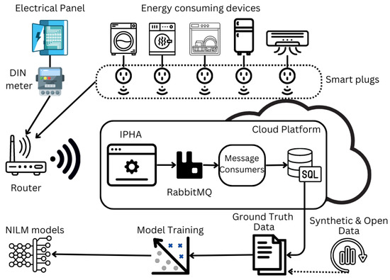
Figure 1.
The data collection pipeline, which has been developed in the framework of the Heart project.
As presented in the Figure 1 and in Table 1, the data sources that have been used for this research can be split into the following categories:

Table 1.
Data sources.
- Heart Data
- Open Data
- Synthetic Data
Heart Data: Among the main contributions of the current study is the public sharing of low-frequency energy consumption data for two households. More specifically, we share the energy consumption data for two Greek households and three devices per each, for a one month period, during summer. More specifically, the first household, named Heart 1, provides the ground truth values for three devices: the washing machine (WM), the fridge (FR), and the iron (IR), as well as the total consumption measurements of the household. The second household, named Heart 2, provides the ground truth values for the WM, the DW, and the FR appliances, along with the total consumption measurements of the household as well. The sampling period that was used in both of the households was 1 second; however, we applied an under-sampling technique, which converts the sampling period to 6 seconds, to be in accordance with the other available datasets.
Open Data: Nowadays, there is a great number of publicly available datasets for NILM [1,56]. In the current research, UK-DALE [57] was used, which contains ground truth and total consumption measurements for five households in the UK for more than four years. It contains measurements for the most common household electrical appliances, and it is one of the go-to datasets for NILM benchmarks. UK-DALE has two versions: one with high- and one with low-frequency measurements. In this study, the low-frequency data were used (6-second sampling period), to match the frequency of the heart data.
Synthetic Data: In order to enhance the analysis of the proposed benchmark and further evaluate our models, we provide a differentiated version of the SynD framework to produce synthetic households with a sampling period of 6 seconds. SynD [15] introduces the concept of employing synthetic datasets as a substitute for costly and lengthy measurement campaigns in NILM for residential buildings. The authors present a synthetic energy dataset consisting of 180 days of synthetic power data for both aggregate and individual appliances. This dataset includes the consumption traces of more than 20 individual appliances, from households located in Austria. In our case, we use these data to create a mixture of real and synthetic data to evaluate the performance of the proposed models. More specifically, we created a mixture of Austrian and Greek households, adding to the SynD pipeline electrical traces both from Austrian and Greek households. We modified the original implementation of SynD to better fit our case study [C3]. We came up with the following changes regarding the randomness factor of the synthetic data generation:
- Consumption Randomness: We slightly modified the function that produces the power level of each appliance.
- Event Randomness: We modified the randomness regarding the appearance of the appliances usage and the intervals of the day in which the usages of the appliances occurred.
The first synthetic household, namely, Heart 3, contains the total consumption measurements of the household and the ground truth values of the DW and the WM. All the devices mentioned have electrical traces of Greek appliances. The second synthetic household, Heart 4, also contains the ground truth values of the same appliances and the total consumption measurements of the household. The electrical traces also originate from Greek household measurements but differ from the traces used for the production of the Heart 3 household. Both households have a total volume of 5 months and contain several appliances that were used as additional noise, which are produced from Austrian appliance traces (SynD dataset).
4. Methodology
The experimental methodology that was followed is described in the following section. Initially, we provide a brief description of the neural networks that were used. Next, a condensed benchmark analysis of the experiments is presented. It should be noted that all the experiments were designed and executed using Torch-NILM [14], an open-source deep learning framework oriented for NILM research. The framework has ready-to-run APIs alongside popular deep learning NILM architectures and data pre-processing methods, including a set of benchmarking cases to compare the networks.
4.1. Deep Learning Topologies
Neural networks learn to solve a task by example, meaning that given an input and the corresponding output, the parameters (weights) of the network are adjusted in order to match the expected output. This process is called training and involves passing the data a number of times through the network to achieve learning. The update of the weights is done using an optimization method based on an algorithm called gradient descent [58]. Due to the mechanics of these algorithms, the data must be given to the network in small parts called the batches. Each time all the training data are passed through the network, an epoch is completed. For all the experiments conducted in the current research, the batch size was set to 1024 and the maximum number of epochs was set to 50, while Adam was used as the optimizer. The hyper parameters for the training of the models are presented in Table 2. More details regarding the training of the networks can be found in the official repository https://github.com/Virtsionis/torch-nilm (accessed on 20 March 2023) of Torch-NILM [14].
Table 2.
Training hyper parameters for all the neural networks.
Energy disaggregation aims to estimate the power consumption of the individual appliances that compose the total (mains) consumption of an installation. During training, both the mains and the appliance consumption time series are given to the model. The appliance data are used as ground truth in order to help the model learn useful patterns and features that belong to the appliance’s electrical signature. After the training is completed, the model can be used for inference, with only the mains consumption of the installation outputting the individual appliance power consumption.
In the current research, five models were used: DAE [3], WGRU [27], S2P [4], NFED [35], and SimpleGRU [60]. DAE is based on an architecture type called the denoising autoencoder, originally proposed by Vincent et al. [61]. The intuition is to extract the clean consumption signal of the target appliance from the mains consumption, which is considered noisy. The model as presented in [3] is composed of three intermediate fully connected layers. Two convolutional layers (CNN) are used in the input and the output of the network as feature extractors. On the other hand, WGRU [27] was based on a recurrent network proposed by Kelly and Knottenbelt [3]. The core element of the network is the bidirectional GRU layer, a more lightweight variation of the recurrent layer [62]. This architecture contains a CNN layer before two serially placed GRUs, following a fully connected layer. The main novelty of this model is that it uses a sliding window approach. The sliding window approach dictates that the total time series is broken into smaller parts of constant length (window) and the network tries to estimate the appliance power consumption of the last point of the window. This way, the network provides one estimate per window, resulting in faster training than using other methods where the network predictions match the input size. For all the experiments, the window size was set to 100 points.
Another approach was followed by Zhang et al. [4], where the proposed model S2P is completely composed of a series of five intermediate CNN layers. Even though S2P contains millions of parameters, the training and inference times are a lot smaller in comparison to the WGRU. This is due to the fact that in CNN layers, many operations are executed in parallel. It should be noted that S2P and WGRU are considered as state-of-the-art models in NILM applications and are expected to be the best-performing ones in this paper also. In an attempt to compensate between size and speed, Nalmpantis et al. [35] designed NFED, an architecture based on FNET [63], a variant of the transformer architecture that uses the Fourier transformation as a feature extractor instead of the attention mechanism. This model consists mainly of fully connected layers and some residual connections, and it is claimed to achieve similar performance to WGRU and S2P models. Finally, SimpleGRU [60] is a more lightweight version of the WGRU that contains only one GRU layer alongside with a smaller CNN layer as feature extractor. This model was used mainly as a baseline model.
4.2. Benchmark Cases
Torch-NILM also contains the benchmark methodology that was proposed by Symeonidis et al. [52]. The benchmark is composed of four categories of experiments that aim to stress test the NILM algorithms gradually, from easy to hard tasks. These categories are described below:
- Single Residence Learning:
- (a)
- Single Residence NILM: Single building NILM is about training and inference on the same house at different time periods. Therefore, the models were evaluated in the same environment where training was executed.
- (b)
- Single Residence Learning and Generalization on Same Dataset: In this case, the training and inference happens on different houses of the same dataset.
The objective of these tests is to measure how well the model can be applied to various types of homes of the same data source. In a nutshell, different homes contain different energy patterns due to a variety of factors, including occupant habits and the use of other electric devices. It is expected that measurements from the same dataset will be similar. In the next chapters, these categories of experiments are notated as Single.
- 2.
- Multi-Residence Learning:
- (a)
- Generalization on same dataset: Contains experiments where the training data are composed of measurements from different homes and testing is applied to unseen homes of the same dataset.
- (b)
- Generalization to Different Datasets: The training data are exactly similar to the above; the testing, though, is applied to unseen homes from other datasets.
It is obvious that the difference between these two categories depend on which datasets the training and testing measurements originate from. The purpose of these experiments is to evaluate the learning capability of models from a variety of sources. Specifically, for the 2(b) category, where the test instances are completely unknown and from a totally different dataset, the challenge for the model naturally increases. These experiments are notated as the Multi category, throughout the paper.
In addition to the benchmarking categories, a fine tuning technique has also been explored. This technique is also know as transfer learning [64], where a pre-trained model on one problem is used as a feature extractor to solve a different one. To use the model to a different domain, its parameters are adjusted by retraining with the data of the new objective. Usually only the last layers of the model are modified, but in this work the entire network was retrained since it was found that it produced better results. Transfer learning is a popular technique in cases of limited data and has been applied in NILM research with some success in [13,31,50].
As presented in Section 3, for the experiments, both synthetic and real measurements were considered. The household appliances that have been selected for the experiments are the following three: (i) DW, (ii) FR, and (iii) WM. The choice of these appliances was not random as these were some common devices available to all of the proposed datasets. Additionally, in order to investigate whether the volume of the data affects the performance of the models, the experiments were executed in two more versions:
- Small volume: The ratio between the data that are used for training and the data that are used for inference is 3:1.
- Large volume: The ratio between the data that are used for training and the data that are used for inference is 4:1.
In the following section, the whole range of experiments, along with the respective findings, is presented in detail.
5. Experiments and Main Findings
The conducted experiments in this study aim to emphasize the distinct aspects of energy disaggregation tasks and optimal methodologies. The following sections provide a detailed account of the experimental design, the corresponding results, and the key discoveries.
5.1. Experimentation Roadmap
Each experiment utilizes the DAE, NFED, S2P, SimpleGRU, and WGRU deep learning architectures, which have been further described in Section 2. As mentioned above, the objective of the experiments is to emphasize on different facets, which can be further used to classify the type of experiments into the three following categories:
- Personalized Models (PM): In this first category of experiments, we focus on fortifying the personalized-ML concept. To achieve this, we experiment on households from the same dataset, both in the training and in the testing procedure. This category involves experiments with households, which originate from all three datasets.
- PM-1: Firstly, we apply our benchmark modeling framework on households included in the open data dataset.
- PM-2: Then, we proceed to the experimentation using the heart data households as our data source.
- PM-3: Finally, we experiment with the synthetic data households mixture.
Generalization Capability (GC): Proceeding to the second group of experiments, we aim to evaluate the generalization capabilities of the benchmark framework. In that direction, we utilize different datasets for the training and inference procedures. We split this case study into two main sub-experiments:
- Train on one: We evaluate the pure generalization capabilities of our models. We conduct two separate sub-experiments for this category.
- (a)
- Open and Heart: In this case, we utilize UK-DALE households from the open dataset for training and the Heart 1, 2 households for testing.
- (b)
- Synthetic and Heart: In the second case, we train our models on Heart 3, 4 of the synthetic dataset, and we use the heart data for inference.
- Train on many: The second main sub-category involves an effort to further enhance the generalization capabilities of our modeling framework by providing a small volume of data from the same dataset both in the training and in the inference procedure. Again, this scenario is further split into two sub-experiments.
- (a)
- Open-Heart and Heart: We utilize households from the open and the heart dataset for training and inference on households only from the heart dataset.
- (b)
- Synthetic-Heart and Heart: In this second case, we use households from the synthetic and the heart dataset for training and only heart data households for inference.
- Fine Tuning Solution (FT): The third main category includes a fine-tuning framework to boost the generalization capabilities of our models. The fine-tuning experimentation is further divided into two sub-categories.
- FT-1: In the first one, we train our models in the UK-DALE households from the open dataset, fine-tune them utilizing Heart 1, 2 from the heart dataset and infer in the latter, whereas in the second one,
- FT-2: We train our models on the synthetic data (Heart 3, 4), fine-tune them on Heart 1, 2, and provide inference results for the same.
At this point, we should also clarify that the following sections do not include a detailed description of all the experiments mentioned above, although all of them have been successfully conducted. More specifically, we have used both the small and the large volume versions for all the experiments, but those described refer only to the best-performing ones. The results of the rest of the experiments are included in Appendix A.
5.2. Personalized Models [PM]
In this first scenario, we utilize the DAE, NFED, S2P, SimpleGRU, and WGRU models using the WM, the DW, and the FR appliances to showcase the personalization capabilities of the benchmarking framework, selecting the same datasets both for training and testing. We segment this scenario into three further sub-scenarios, namely, PM-1, PM-2, and PM-3, as mentioned in the experimentation roadmap. PM-1 and PM-2 are single and small-volume experiments, whereas PM-3 is a multi- and large-volume experiment.
PM-1: In this experiment, we trained and tested our models utilizing data from the UK-DALE dataset. More specifically, we utilized 3 months of training and 1 month of testing on “UK-DALE 1”. The examined appliances are the WM, the FR, and the DW.
From Figure 2, it seems that the benchmarking framework achieves the best event detection results in the WM and the FR appliances, whereas, in the case of the DW appliance, it achieves relatively low F1-scores below 40%. In terms of MAE, all the models seem to achieve good results, below the value of 10, in the WM, whereas in the FR and the DW experiments, the MAE is increased in the range [15, 25]. Overall, the models achieve decent results both in event detection and energy prediction, with the WM appliance and the WGRU model demonstrating the best results in the current experiment.
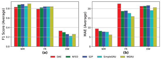
Figure 2.
PM-1 results for the models DAE, NFED, S2P, SimpleGRU, and WGRU for the WM, the FR, and the DW, utilizing UK-DALE 1 household for training and inference: (a,b) F1-score and MAE results.
PM-2: After we evaluated the personalization capabilities of our models in the Open data in the PM-1 experiment, we proceeded to the PM-2 experiment involving the heart data. Here, the examined appliances are the WM and the FR. We utilized 3 weeks of the Heart 1 household for training and 1 week of Heart 1 for testing.
As depicted in Figure 3, our models achieve better event detection in the FR appliance, with F1-scores over 80%, whereas in the WM appliance, only the NFED and S2P models achieve an F1-score over 70%. In terms of MAE, all the models in both appliances achieve great results in the range [10, 15]. In conclusion, the most solid model among the two appliances in terms of event detection and energy prediction was the S2P model, with the NFED following closely.
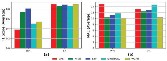
Figure 3.
PM-2 results for the models DAE, NFED, S2P, SimpleGRU, and WGRU for the WM and the FR utilizing Heart 1 household for training and inference: (a,b) F1-score and MAE results.
PM-3: We conclude the personalized models category of experiments with the synthetic data households mixture. Here, the appliances involved are the DW and the WM. We use 2 months of “Heart 3” and 2 months of “Heart 4” for training and 1 month of “Heart 3” and 1 month of “Heart 4” for testing.
The S2P and WGRU seem to be the best-performing models, as presented in Figure 4, both in terms of event detection and energy prediction. Both achieve a MAE score lower than 5 in the WM appliance and over 80% in the event detection of the WM appliance. Generally, all the models, except DAE, achieve good results both in terms of F1-score and MAE metrics. Comparing the current experiment with the PM-1 and PM-2 scenarios, we conclude that the easier-to-predict nature of synthetic data in comparison to the real data helps our benchmarking framework to interpret the trends in the data and boost its overall performance.
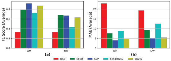
Figure 4.
PM-3 results for the models DAE, NFED, S2P, SimpleGRU, WGRU for the WM and DW, utilizing “Heart 3” and “Heart 4” households for training and Heart 4 for inference: (a,b) F1-score and MAE results.
5.3. Genaralization Capability (GC)
Following the evaluation of the personalized-ML concept of our proposed benchmark, we proceed to inspect the generalization capabilities of our models. Although the concept of personalization is solid in the NILM area and the generalization capabilities of the proposed architectures encounter several difficulties, we propose a way to improve the generalization capabilities of our models. In this section, we first examine the pure generalization capabilities of the proposed deep learning architectures by training our models in one dataset and evaluating them in another. Secondly, we add a small chunk of the dataset in which we infer in the training volume of data to enhance the training of the models.
Train on one—Open and Heart: In this experiment, the models were trained using data only from the UK-DALE data set and tested on data from heart installations. We considered 3 months for training in “UK-DALE 1” and 1 month for inference in “Heart 2”. The appliances of interest are the WM, the FR, and the DW. The goal of this simulation is to quantify the GC of the models and whether this setting can be used for real-world use cases, where the models are tested on unseen data.
In Figure 5, we observe that all models have difficulties in event detection in all three appliances achieving low F1-scores below 27%. In terms of MAE, the results are decent only in the WM appliance, whereas in the FR and DW appliances, the predicted energy values deviate significantly from the actual ones resulting in high MAE scores. As a general conclusion, we can say that the current experiment reveals the generalization difficulties of our benchmarking framework.
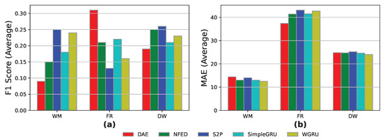
Figure 5.
Train on one—open and heart results for the models DAE, NFED, S2P, SimpleGRU, and WGRU for the WM, the FR, and the DW, utilizing “UK-DALE 1” household for training and “Heart 2” household for testing: (a,b) F1-score and MAE results.
Train on one—synthetic and heart: In this case study, the models were trained using data only from the synthetic data set and tested on the heart data. More specifically, we used 4 months for training on “Heart 4” and 1 month for inference on “Heart 2” household. The appliances of interest are the WM and the DW.
As depicted in Figure 6, the WGRU model achieved the best event detection with over 70% on the WM appliance, with the S2P following as the second best with a decent F1-score over 60%. Also in terms of MAE in the WM appliance, the NFED, S2P, and WGRU models achieve an MAE score below 15. In the DW appliance, all the models achieve decent results both in terms of event detection and energy prediction.
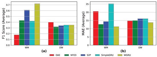
Figure 6.
Train on one—synthetic and heart results for the models DAE, NFED, S2P, SimpleGRU, and WGRU for the WM and the DW, utilizing “Heart 4” household for training and “Heart 2” household for testing: (a,b) F1-score and MAE results.
As an overall conclusion, we state that the generalization capabilities of our models increased significantly in comparison with the previous open and heart experiment. This is justified because the synthetic data in which our models were trained utilize traces from the heart data that we used for inference.
Train on many—Open-Heart and Heart: This scenario utilizes training data from “UK-DALE 1” and “Heart 1 & 2” installations, whereas the inference occurs on “Heart 2”. More specifically, we utilize three months from the “UK-DALE 1”, 15 days from “Heart 1”, and 15 days from “Heart 2” for training and 15 days from “Heart 2” for inference. The idea is that given only a small number of data from the target installation, a part of it can be used for training in combination with publicly available data. This way, the network will receive useful information from the target installation without the risk of overfitting.
As shown in Figure 7, the WGRU model achieves the best F1-score for the WM and the FR and the lowest MAE score for all the appliances. The S2P model achieved almost 60% in the DW appliance event detection, which is the highest score. Regarding the MAE metric, the models perform better than the train on one—open and heart case study for the WM and almost on par for the DW.
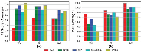
Figure 7.
Train on many—open-heart and heart results for the models DAE, NFED, S2P, SimpleGRU, and WGRU for the WM, the FR, and the DW, utilizing UK-DALE 1 and Heart 1 and 2 households for training and Heart 2 household for testing: (a,b) F1-score and MAE results.
Overall, the performance boost for all the models and appliances is notable in comparison with the train on one—open and heart case study. This fact proves the point that adding a small chunk of the data, from which we infer in the training data volume, significantly improves the performance of the models.
Train on many—Synthetic-Heart and Heart: This case study investigates a similar multi-category experiment use case with the previous train on many—open-heart and heart experiment, with the difference being using synthetic households instead of open. We utilize 2 months of “Heart 4”, 15 days of “Heart 1”, and 15 days of “Heart 2” for training, as well as 15 days of “Heart 2” for testing. This scenario can be used in real-world situations where data from publicly available sources cannot be used. Since the synthetic data contains traces from Greek houses only for the appliances of interest, a performance boost is expected.
As presented in Figure 8, and in comparison to the previous case study, namely, train on many—open-heart and heart, for the WM appliance, the best-performing models WGRU and S2P show an increase of about 10% in F1-score, with the WGRU scoring almost 80%. In terms of the DW appliance event detection, the performance of the models is similar but a bit lower than the case train on many—open-heart and heart. Regarding the MAE, the WGRU is the winner for both appliances performing on par with the previous case study. It should be noted that the S2P model showed the greatest improvement, reducing the error for both appliances.
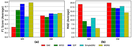
Figure 8.
Train on many—synthetic-heart and heart results for the models DAE, NFED, S2P, SimpleGRU, and WGRU for the WM and the DW, utilizing Heart 1, 2, and 4 households for training and Heart 2 household for testing: (a,b) F1-score and MAE results.
We conclude that, for the current experiment, we observe that this scenario outperforms all the previous GC scenarios. This occurs because the training set has been extended with a small chunk of data that will be used for inference and contains traces similar to those of the appliances of interest.
5.4. Fine Tuning Solution
The logic behind this case study is quite similar to the GC case. In order to enhance the performance of the models, a combination of data from various datasets is used during training. Additionally, a small number of data from the target installation are incorporated to help the models learn useful patterns specifically from the target household. The datasets are combined using a technique called fine-tuning or transfer learning. This method uses a pre-trained model from one domain fine-tuned to a different one. Fine-tuning involves retraining the model on the new domain data. In the current research, the models are trained on one NILM dataset and fine-tuned on the target installation. The intuition behind this method is that the model has already learned the problem of NILM and the basic appliance features and is then fine-grained with data of different households.
Open-heart and heart: In this scenario, the models are trained on “UK-DALE 1” installation for four months. Then, 3 weeks of the Heart 2 measurements are used for fine-tuning and 1 week for testing. The results in Figure 9 show that for the WM, the S2P achieves almost 81% in F1-score, better than the best-performing model of the previous GC case study. For the DW, the models perform worse than the best-performing model of the GC case study, with the best-performing DAE achieving 50% on the F1-metric. The MAE errors are similar to the train on many—synthetic-heart and heart case study.
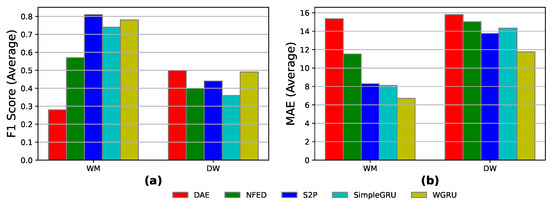
Figure 9.
Open-heart and heart results for the models DAE, NFED, S2P, SimpleGRU, and WGRU for the WM and the DW, utilizing UK-DALE 1 for training and Heart 2 for fine-tuning and inference: (a,b) F1-score and MAE results.
Synthetic-heart and heart: Here, data from the synthetic houses were used for the training instead of UK-DALE. More specifically, the models are trained on “Heart 4” installation for four months. Then, 3 weeks of the “Heart 2” measurements are used for fine-tuning and 1 week for testing. As shown in Figure 10, the results for “Heart 2” are better than the previous open-heart and heart fine-tuning solution for both appliances, with better F1-scores for the best-performing models and lower MAE errors. This happens due to the fact that data from the same dataset (heart) was used for training and fine-tuning. Hence, the models learn similar features due to the similar electrical traces of the data used for training and for inference.
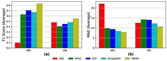
Figure 10.
Synthetic-heart and heart results for the models DAE, NFED, S2P, SimpleGRU, and WGRU for the WM and the DW, utilizing “Heart 4” for training and “Heart 2” for fine-tuning and inference: (a,b) F1-score and MAE results.
5.5. Main Findings
To facilitate a more direct comparison between the different experimentation scenarios, we generated Figure 11. There, we present the performance of the best-performing models in each experiment in terms of F1-score and MAE score for the WM and the DW appliances. We selected the current devices because they co-exist in all the experimentation scenarios except for the PM-2 experiment, which is not present in the current figure for this exact reason. The FR appliance was also not selected since it is not involved in several experiments.
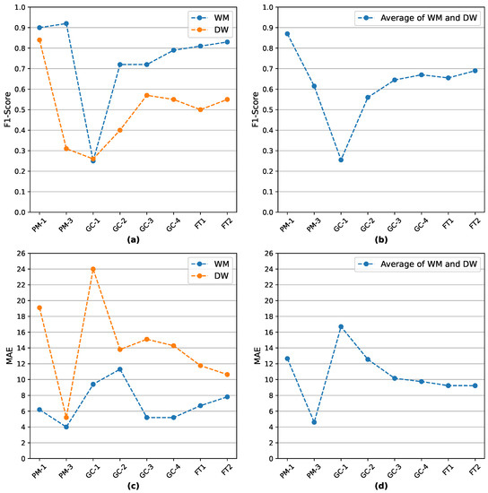
Figure 11.
Highest recorded F1-scores and lowest recorded MAE scores for the experiments in which the WM and DW appliances were involved: (a) highest recorded F1-scores for the WM and DW per experiment, (b) average of the highest recorded F1-scores between the WM and DW per experiment, (c) lowest recorded MAE scores for the WM and DW per experiment, and (d) average of the lowest recorded MAE between the WM and DW per experiment.
The main conclusions from Figure 11 are, firstly, the strong personalization character of the best-performing models (C1) and, secondly, the enhancing of their generalization capabilities via the fine-tuning framework (C2). The first point can be justified by the fact that the PM-1 experiment records the highest F1-score among all the experiments and a significantly lower MAE error. Regarding the second point, it is explained by the fact that the FT2 experiment achieves the lowest MAE score and the highest F1-score among the (FT) and GC experiments.
Furthermore, after a detailed revision of the results of the different experimentation scenarios in the current study, the following key points can be raised:
- The models perform and generalize better in cases where the training happens on data from one house and the inference is executed on data coming from houses of the same dataset. Conducting experiments with training data from multiple households from the same datasets produced worse results than the single-category experiments (C1).
- The (FT) solution produces better results than the GC experiments in almost all cases while enhancing the generalization capabilities of our models at a higher degree (C2).
- Another observation for the GC and (FT) experiments is the following: for the DW appliance, the models perform better in situations where we use Synthetic data for training. On the other hand, in the case of the WM appliance training with open data produced better results. This may mean that either the quality of the used data is different for those appliances or that their operation from the users fits better the target country. For example, it is possible that the UK (open data) people use the WM similarly to users in Greece (heart data) (the same programs, a similar hour of the day for operation, etc.).
- As presented, the models WGRU and S2P are the most robust models in this study, being the best-performing models in almost all the experiments. Given their characteristics (size, training/inference time), one can choose among the two for a real-world disaggregation application, similar to the investigated scenarios.
- Finally, combining all the previous points, we can reach a more generic conclusion. Considering the cost and time restrictions of collecting a large number of data in the NILM domain, a cost- and time-efficient strategy is very important. Our approach focuses on that specific point: producing synthetic data to cover the data shortage issue and at the same time achieves decent performance with the fine tuning solution (C2). As a result, we can state that we provide a high-performing cost-effective solution in the NILM community, which will have a high impact on real-life data, time, or funding shortage scenarios.
At this point, we should also highlight that personalized ML and generalization are often considered contradictory terms. However, we would like to emphasize that in this paper’s context, generalization refers to enhancing the performance and applicability of the models beyond their initial training conditions. While personalized models perform better in capturing individual consumption patterns, they may face challenges when applied to unseen scenarios or users. To address this limitation, we have proposed a two-fold strategy for generalization. First, we employed fine-tuning techniques to adapt the personalized models to new instances, allowing them to perform well in varying contexts. Secondly, we incorporated synthetic data to augment the training dataset. This enables our models to learn from a broader range of consumption patterns, even those not present in the original dataset. By leveraging synthetic data, we aim to enhance the generalization capabilities of our models, enabling them to make accurate predictions in scenarios beyond the training set. Therefore, in our research, the term generalization refers to the ability of our models to adapt and perform well in new contexts through fine-tuning and the utilization of synthetic data. We have shown that this approach strikes a balance between personalization and generalization, providing improved performance while maintaining the ability to generalize to unseen situations.
6. Conclusions and Future Work
NILM analyzes the energy usage of individual electrical devices within a building or household. This technique involves the monitoring of the overall power consumption and utilization of signal processing techniques to disaggregate the power signal into individual device-level power profiles. In this paper, we propose HeartDIS, a generalizable end-to-end energy disaggregation pipeline, based on a wide range of experiments both at data and methodology level.
In terms of data, we utilize various realistic and synthetic data sources. Besides UK-DALE households, which are extensively utilized in the literature, namely, open data, we support the open NILM community by providing data of two Greek households, named heart data. Furthermore, we produce a slightly automated and alternated version of the SynD framework that suits better our case study, and we produce two synthetic households, which we also present to the community, named synthetic data. In terms of models, we utilize the open-source Torch-NILM framework, which contains several popular deep-learning architectures.
The main scope of the current paper is to prove the personalized nature of the bench-marking framework and to test the generalization capabilities of the models. The first point is fortified through the personalized models (PM) experiments. The second point is tested through the GC and FT experiments. Both enhance the generalization capabilities of the models, with the latter achieving overall the best results. Finally, a more general conclusion from the overall experimentation procedure is that the performance of the models is device and dataset oriented. In other words, different models achieve the best results in different case studies and different datasets. Nevertheless, we can state that the S2P and the WGRU models were the best-performing for most of the scenarios.
Regarding future work, taking into account the importance of data privacy in the context of personalized ML for NILM, further experimentation with privacy-preserving ML techniques for NILM will be conducted. In our study, we have conducted experiments utilizing transfer learning techniques, but further research should be considered regarding the important aspect of privacy preservation, particularly from a differential privacy perspective with techniques such as federated learning. These privacy-centric approaches will further enhance the integrity and ethical considerations of our work.
Author Contributions
Conceptualization, I.D., A.V. and C.A.; methodology, I.D. and N.V.G.; software, N.V.G. and N.G.; validation, I.D., C.B. and N.V.G.; formal analysis, I.D. and N.V.G.; investigation, N.G. and N.V.G.; resources, A.V.; data curation, N.G., C.A., C.B. and N.V.G.; writing—original draft preparation, N.G., N.V.G. and I.D.; writing—review and editing, N.V.G., I.D. and C.A.; visualization, N.G., N.V.G. and I.D.; supervision, I.D. and A.V.; project administration, A.V.; and funding acquisition, A.V. All authors have read and agreed to the published version of the manuscript.
Funding
This research is co-financed by Greece and European Union through the Operational Program Competitiveness, Entrepreneurship, and Innovation under the call RESEARCHCREATE-INNOVATE (project T2EDK-03898).
Data Availability Statement
We share our data with the scientific community. You can find the data for our study at the following link: https://github.com/Datalab-AUTH/Heart-Synd (accessed on 20 March 2023).
Conflicts of Interest
The authors declare no conflict of interest.
Abbreviations
The following abbreviations are used in this manuscript:
| GC | Generalization capability |
| FT | Fine-tuning |
| WM | Washing machine |
| DW | Dishwasher |
| FR | Fridge |
| ML | Machine learning |
| EU | European Union |
| NILM | Non-intrusive load monitoring |
| IoT | Internet of things |
| PM | Personalized models |
| MAE | Mean average error |
Appendix A
Table A1.
Performance comparison for the PM-1 experiment for the WM considering open data as the data source. The best results are highlighted in bold.
Table A1.
Performance comparison for the PM-1 experiment for the WM considering open data as the data source. The best results are highlighted in bold.
| Device | Cat. | Vol. | Train | Test | Model | F1s | RETE | MAE |
|---|---|---|---|---|---|---|---|---|
| WM | Single | Small | UK-DALE 1 | UK-DALE 1 | DAE | 0.83 | 0.07 | 9.4 |
| NFED | 0.88 | 0.05 | 8.2 | |||||
| S2P | 0.89 | 0.05 | 7.8 | |||||
| SimpleGRU | 0.85 | 0.03 | 7.7 | |||||
| WGRU | 0.9 | 0.03 | 6.2 | |||||
| WM | Single | Small | UK-DALE 1 | UK-DALE 2 | DAE | 0.18 | 0.7 | 10.7 |
| NFED | 0.37 | 0.94 | 11 | |||||
| S2P | 0.65 | 0.81 | 10 | |||||
| SimpleGRU | 0.5 | 0.68 | 12.4 | |||||
| WGRU | 0.65 | 0.84 | 10 | |||||
| WM | Single | Small | UK-DALE 1 | UK-DALE 4 | DAE | 0.29 | 0.08 | 35.4 |
| NFED | 0.37 | 0.18 | 32.7 | |||||
| S2P | 0.47 | 0.15 | 23.2 | |||||
| SimpleGRU | 0.42 | 0.24 | 27.8 | |||||
| WGRU | 0.5 | 0.19 | 26.4 | |||||
| WM | Single | Small | UK-DALE 1 | UK-DALE 5 | DAE | 0.22 | 0.82 | 42.5 |
| NFED | 0.4 | 0.85 | 44.1 | |||||
| S2P | 0.56 | 0.79 | 42.7 | |||||
| SimpleGRU | 0.42 | 0.72 | 45.3 | |||||
| WGRU | 0.47 | 0.78 | 44.8 | |||||
| WM | Multi | Small | UK-DALE 1, 5 | UK-DALE 1 | DAE | 0.6 | 0.11 | 20.3 |
| NFED | 0.81 | 0.08 | 11.8 | |||||
| S2P | 0.84 | 0.05 | 11.1 | |||||
| SimpleGRU | 0.81 | 0.05 | 10.4 | |||||
| WGRU | 0.87 | 0.05 | 9.3 | |||||
| WM | Multi | Small | UK-DALE 1, 5 | UK-DALE 2 | DAE | 0.16 | 0.26 | 17.1 |
| NFED | 0.29 | 0.68 | 11.7 | |||||
| S2P | 0.43 | 0.71 | 12.2 | |||||
| SimpleGRU | 0.38 | 0.68 | 12.3 | |||||
| WGRU | 0.57 | 0.76 | 10.7 | |||||
| WM | Multi | Small | UK-DALE 1, 5 | UK-DALE 4 | DAE | 0.24 | 0.28 | 44.2 |
| NFED | 0.33 | 0.17 | 33.5 | |||||
| S2P | 0.37 | 0.28 | 26.2 | |||||
| SimpleGRU | 0.42 | 0.09 | 23.8 | |||||
| WGRU | 0.41 | 0.29 | 24.4 | |||||
| WM | Multi | Small | UK-DALE 1, 5 | UK-DALE 5 | DAE | 0.39 | 0.16 | 32.2 |
| NFED | 0.67 | 0.24 | 27.6 | |||||
| S2P | 0.64 | 0.22 | 28.4 | |||||
| SimpleGRU | 0.63 | 0.22 | 28.2 | |||||
| WGRU | 0.68 | 0.28 | 25.7 |
Table A2.
Performance comparison for the PM-1 experiment for the DW and the FR considering open data as the data source.The best results are highlighted in bold.
Table A2.
Performance comparison for the PM-1 experiment for the DW and the FR considering open data as the data source.The best results are highlighted in bold.
| Device | Cat. | Vol. | Train | Test | Model | F1s | RETE | MAE |
|---|---|---|---|---|---|---|---|---|
| DW | Single | Small | UK-DALE 1 | UK-DALE 1 | DAE | 0.33 | 0.57 | 21.3 |
| NFED | 0.3 | 0.54 | 21.4 | |||||
| S2P | 0.26 | 0.52 | 21.7 | |||||
| SimpleGRU | 0.22 | 0.39 | 19.1 | |||||
| WGRU | 0.26 | 0.47 | 20.6 | |||||
| DW | Single | Small | UK-DALE 1 | UK-DALE 2 | DAE | 0.64 | 0.1 | 17 |
| NFED | 0.67 | 0.2 | 15.7 | |||||
| S2P | 0.64 | 0.19 | 15.7 | |||||
| SimpleGRU | 0.58 | 0.2 | 15.9 | |||||
| WGRU | 0.69 | 0.17 | 15.1 | |||||
| DW | Single | Small | UK-DALE 1 | UK-DALE 5 | DAE | 0.38 | 0.68 | 49.7 |
| NFED | 0.29 | 0.75 | 68.1 | |||||
| S2P | 0.33 | 0.58 | 42.5 | |||||
| SimpleGRU | 0.28 | 0.53 | 41 | |||||
| WGRU | 0.38 | 0.47 | 36.4 | |||||
| DW | Multi | Small | UK-DALE 1, 2 | UK-DALE 1 | DAE | 0.38 | 0.26 | 10.6 |
| NFED | 0.24 | 0.17 | 7.4 | |||||
| S2P | 0.34 | 0.08 | 7.3 | |||||
| SimpleGRU | 0.25 | 0.14 | 8.1 | |||||
| WGRU | 0.3 | 0.17 | 6.7 | |||||
| DW | Multi | Small | UK-DALE 1, 2 | UK-DALE 2 | DAE | 0.65 | 0.15 | 19 |
| NFED | 0.52 | 0.19 | 17.7 | |||||
| S2P | 0.56 | 0.29 | 20 | |||||
| SimpleGRU | 0.51 | 0.25 | 19.6 | |||||
| WGRU | 0.47 | 0.14 | 18.4 | |||||
| DW | Multi | Small | UK-DALE 1, 2 | UK-DALE 5 | DAE | 0.39 | 0.58 | 36.6 |
| NFED | 0.19 | 0.71 | 65.4 | |||||
| S2P | 0.27 | 0.49 | 43.3 | |||||
| SimpleGRU | 0.25 | 0.23 | 30.9 | |||||
| WGRU | 0.26 | 0.3 | 31.4 | |||||
| FR | Single | Small | UK-DALE 1 | UK-DALE 1 | DAE | 0.79 | 0.12 | 22.6 |
| NFED | 0.82 | 0.11 | 18.7 | |||||
| S2P | 0.84 | 0.12 | 18.9 | |||||
| SimpleGRU | 0.84 | 0.09 | 17.6 | |||||
| WGRU | 0.84 | 0.11 | 15.9 | |||||
| FR | Single | Small | UK-DALE 1 | UK-DALE 2 | DAE | 0.82 | 0.1 | 21.1 |
| NFED | 0.82 | 0.17 | 22.2 | |||||
| S2P | 0.82 | 0.16 | 22.1 | |||||
| SimpleGRU | 0.83 | 0.19 | 21.3 | |||||
| WGRU | 0.82 | 0.2 | 20.4 | |||||
| FR | Single | Small | UK-DALE 1 | UK-DALE 4 | DAE | 0.68 | 0.35 | 29.4 |
| NFED | 0.61 | 0.21 | 32.4 | |||||
| S2P | 0.54 | 0.15 | 35.1 | |||||
| SimpleGRU | 0.58 | 0.18 | 32.5 | |||||
| WGRU | 0.56 | 0.08 | 31 | |||||
| FR | Multi | Small | UK-DALE 1, 2 | UK-DALE 1 | DAE | 0.76 | 0.14 | 25 |
| NFED | 0.81 | 0.14 | 21 | |||||
| S2P | 0.81 | 0.13 | 21 | |||||
| SimpleGRU | 0.81 | 0.14 | 20.2 | |||||
| WGRU | 0.83 | 0.14 | 18.7 | |||||
| FR | Multi | Small | UK-DALE 1, 2 | UK-DALE 2 | DAE | 0.83 | 0.07 | 18.2 |
| NFED | 0.85 | 0.09 | 16.7 | |||||
| S2P | 0.85 | 0.11 | 17.6 | |||||
| SimpleGRU | 0.84 | 0.12 | 16.5 | |||||
| WGRU | 0.86 | 0.11 | 15.2 | |||||
| FR | Multi | Small | UK-DALE 1, 2 | UK-DALE 4 | DAE | 0.68 | 0.34 | 30.4 |
| NFED | 0.6 | 0.21 | 31.4 | |||||
| S2P | 0.53 | 0.14 | 34.1 | |||||
| SimpleGRU | 0.61 | 0.2 | 30.8 | |||||
| WGRU | 0.57 | 0.11 | 30 |
Table A3.
Performance comparison for the PM-2 case study for the WM, the FR, and the DW, utilizing heart data as data source.The best results are highlighted in bold.
Table A3.
Performance comparison for the PM-2 case study for the WM, the FR, and the DW, utilizing heart data as data source.The best results are highlighted in bold.
| Device | Cat. | Vol. | Train | Test | Model | F1s | RETE | MAE |
|---|---|---|---|---|---|---|---|---|
| WM | single | small | Heart 1 | Heart 1 | DAE | 0.38 | 0.53 | 14.8 |
| NFED | 0.74 | 0.21 | 10.4 | |||||
| S2P | 0.81 | 0.24 | 11.2 | |||||
| SimpleGRU | 0.5 | 0.26 | 11.7 | |||||
| WGRU | 0.54 | 0.34 | 10.1 | |||||
| WM | Single | Small | Heart 1 | Heart 2 | DAE | 0.26 | 0.45 | 13.2 |
| NFED | 0.3 | 0.68 | 12.1 | |||||
| S2P | 0.4 | 0.56 | 12.8 | |||||
| SimpleGRU | 0.31 | 0.7 | 12.4 | |||||
| WGRU | 0.25 | 0.76 | 11.8 | |||||
| WM | Multi | Large | Heart 1, 2 | Heart 1 | DAE | 0.28 | 0.13 | 12.9 |
| NFED | 0.58 | 0.27 | 9.6 | |||||
| S2P | 0.65 | 0.22 | 8.9 | |||||
| SimpleGRU | 0.37 | 0.25 | 10.5 | |||||
| WGRU | 0.48 | 0.22 | 8.6 | |||||
| WM | Multi | Large | Heart 1, 2 | Heart 2 | DAE | 0.24 | 0.12 | 14.7 |
| NFED | 0.6 | 0.14 | 9.5 | |||||
| S2P | 0.62 | 0.21 | 10 | |||||
| SimpleGRU | 0.31 | 0.26 | 12.4 | |||||
| WGRU | 0.44 | 0.25 | 9.3 | |||||
| FR | Single | Small | Heart 1 | Heart 1 | DAE | 0.9 | 0.01 | 13.1 |
| NFED | 0.86 | 0.03 | 12.4 | |||||
| S2P | 0.89 | 0.05 | 12.8 | |||||
| SimpleGRU | 0.86 | 0.04 | 14.6 | |||||
| WGRU | 0.9 | 0.03 | 10.4 | |||||
| FR | Single | Small | Heart 1 | Heart 2 | DAE | 0.34 | 0.67 | 28.6 |
| NFED | 0.34 | 0.67 | 30.1 | |||||
| S2P | 0.4 | 0.68 | 29.3 | |||||
| SimpleGRU | 0.36 | 0.6 | 26.3 | |||||
| WGRU | 0.4 | 0.68 | 29.3 | |||||
| FR | Multi | Large | Heart 1, 2 | Heart 1 | DAE | 0.86 | 0.13 | 15.9 |
| NFED | 0.89 | 0.08 | 13.1 | |||||
| S2P | 0.89 | 0.1 | 15.5 | |||||
| SimpleGRU | 0.89 | 0.11 | 14 | |||||
| WGRU | 0.9 | 0.11 | 12 | |||||
| FR | Multi | Large | Heart 1, 2 | Heart 2 | DAE | 0.53 | 0.13 | 13.4 |
| NFED | 0.7 | 0.08 | 12.1 | |||||
| S2P | 0.71 | 0.1 | 13.3 | |||||
| SimpleGRU | 0.7 | 0.11 | 12.3 | |||||
| WGRU | 0.72 | 0.11 | 12.3 | |||||
| DW | Single | Small | Heart 2 | Heart 2 | DAE | 0.45 | 0.27 | 16.2 |
| NFED | 0.38 | 0.16 | 12.9 | |||||
| S2P | 0.5 | 0.09 | 11 | |||||
| SimpleGRU | 0.48 | 0.18 | 10.2 | |||||
| WGRU | 0.5 | 0.19 | 9.9 |
Table A4.
Performance comparison for the PM-3 case study for the WM, the FR, and the DW, utilizing synthetic data as data source.The best results are highlighted in bold.
Table A4.
Performance comparison for the PM-3 case study for the WM, the FR, and the DW, utilizing synthetic data as data source.The best results are highlighted in bold.
| Device | Cat. | Vol. | Train | Test | Model | F1s | RETE | MAE |
|---|---|---|---|---|---|---|---|---|
| WM | Multi | Large | Heart 3, 4 | Heart 3 | DAE | 0.27 | 0.46 | 15.6 |
| NFED | 0.72 | 0.08 | 5.2 | |||||
| S2P | 0.83 | 0.06 | 2.8 | |||||
| SimpleGRU | 0.62 | 0.17 | 6.1 | |||||
| WGRU | 0.81 | 0.1 | 3.5 | |||||
| WM | Multi | Large | Heart 3, 4 | Heart 4 | DAE | 0.33 | 0.12 | 22.9 |
| NFED | 0.79 | 0.12 | 7.6 | |||||
| S2P | 0.92 | 0.05 | 4 | |||||
| SimpleGRU | 0.72 | 0.08 | 8.8 | |||||
| WGRU | 0.87 | 0.06 | 4.7 | |||||
| DW | Multi | Large | Heart 3,4 | Heart 3 | DAE | 0.3 | 0.22 | 17.7 |
| NFED | 0.52 | 0.1 | 10.1 | |||||
| S2P | 0.57 | 0.07 | 7.1 | |||||
| SimpleGRU | 0.57 | 0.21 | 11.3 | |||||
| WGRU | 0.55 | 0.13 | 7.5 | |||||
| DW | Multi | Large | Heart 3, 4 | Heart 4 | DAE | 0.33 | 0.19 | 19.3 |
| NFED | 0.68 | 0.07 | 9.2 | |||||
| S2P | 0.67 | 0.05 | 5.2 | |||||
| SimpleGRU | 0.43 | 0.14 | 12.5 | |||||
| WGRU | 0.63 | 0.03 | 5.4 |
Table A5.
Performance comparison for the train on one—open and heart case study for the WM, the FR, and the DW, utilizing open data for training and heart data for testing.The best results are highlighted in bold.
Table A5.
Performance comparison for the train on one—open and heart case study for the WM, the FR, and the DW, utilizing open data for training and heart data for testing.The best results are highlighted in bold.
| Device | Cat. | Vol. | Train | Test | Model | F1s | RETE | MAE |
|---|---|---|---|---|---|---|---|---|
| WM | Single | Small | UK-DALE 1 | Heart 1 | DAE | 0.15 | 0.8 | 13.4 |
| NFED | 0.4 | 0.71 | 12.3 | |||||
| S2P | 0.73 | 0.56 | 11.3 | |||||
| SimpleGRU | 0.65 | 0.54 | 9.4 | |||||
| WGRU | 0.63 | 0.59 | 10.1 | |||||
| WM | Single | Small | UK-DALE 1 | Heart 2 | DAE | 0.09 | 0.84 | 14.4 |
| NFED | 0.15 | 0.86 | 13 | |||||
| S2P | 0.25 | 0.8 | 14 | |||||
| SimpleGRU | 0.18 | 0.79 | 13 | |||||
| WGRU | 0.24 | 0.7 | 12.5 | |||||
| WM | Single | Large | UK-DALE 1 | Heart 1 | DAE | 0.15 | 0.55 | 13.4 |
| NFED | 0.35 | 0.67 | 12.7 | |||||
| S2P | 0.66 | 0.59 | 12.1 | |||||
| SimpleGRU | 0.56 | 0.66 | 11.5 | |||||
| WGRU | 0.61 | 0.6 | 11.2 | |||||
| WM | Single | Large | UK-DALE 1 | Heart 2 | DAE | 0.14 | 0.59 | 15.9 |
| NFED | 0.24 | 0.89 | 14.1 | |||||
| S2P | 0.3 | 0.71 | 16.9 | |||||
| SimpleGRU | 0.22 | 0.84 | 15.2 | |||||
| WGRU | 0.29 | 0.86 | 14.9 | |||||
| FR | Single | Small | UK-DALE 1 | Heart 1 | DAE | 0.68 | 0.04 | 20.6 |
| NFED | 0.75 | 0.89 | 22 | |||||
| S2P | 0.71 | 0.07 | 23.3 | |||||
| SimpleGRU | 0.61 | 0.84 | 24.8 | |||||
| WGRU | 0.61 | 0.25 | 24.7 | |||||
| FR | Single | Small | UK-DALE 1 | Heart 2 | DAE | 0.31 | 0.76 | 37.4 |
| NFED | 0.21 | 0.87 | 41.4 | |||||
| S2P | 0.13 | 0.89 | 43.1 | |||||
| SimpleGRU | 0.22 | 0.87 | 41.5 | |||||
| WGRU | 0.16 | 0.9 | 42.7 | |||||
| FR | Single | Large | UK-DALE 1 | Heart 1 | DAE | 0.67 | 0.4 | 23.1 |
| NFED | 0.74 | 0.1 | 23.3 | |||||
| S2P | 0.64 | 0.1 | 26 | |||||
| SimpleGRU | 0.64 | 0.07 | 26.7 | |||||
| WGRU | 0.65 | 0.16 | 24.8 | |||||
| FR | Single | Large | UK-DALE 1 | Heart 2 | DAE | 0.26 | 0.76 | 40.3 |
| NFED | 0.21 | 0.87 | 43.9 | |||||
| S2P | 0.12 | 0.88 | 44.6 | |||||
| SimpleGRU | 0.28 | 0.76 | 39.7 | |||||
| WGRU | 0.12 | 0.91 | 45.4 | |||||
| DW | Single | Small | UK-DALE 1 | Heart 2 | DAE | 0.19 | 0.64 | 24.8 |
| NFED | 0.25 | 0.74 | 24.7 | |||||
| S2P | 0.26 | 0.78 | 25.2 | |||||
| SimpleGRU | 0.21 | 0.82 | 24.6 | |||||
| WGRU | 0.23 | 0.82 | 24 | |||||
| DW | Single | Large | UK-DALE 1 | Heart 2 | DAE | 0.13 | 0.72 | 28.2 |
| NFED | 0.26 | 0.67 | 28 | |||||
| S2P | 0.23 | 0.77 | 30.3 | |||||
| SimpleGRU | 0.13 | 0.77 | 33.8 | |||||
| WGRU | 0.17 | 0.81 | 27.8 |
Table A6.
Performance comparison for the train on one—synthetic and heart case study for the WM and DW, utilizing synthetic data for training and heart data for inference.The best results are highlighted in bold.
Table A6.
Performance comparison for the train on one—synthetic and heart case study for the WM and DW, utilizing synthetic data for training and heart data for inference.The best results are highlighted in bold.
| Device | Cat. | Vol. | Train | Test | Model | F1s | RETE | MAE |
|---|---|---|---|---|---|---|---|---|
| WM | Single | Large | Heart 4 | Heart 1 | DAE | 0.23 | 0.16 | 20.5 |
| NFED | 0.21 | 0.22 | 23.3 | |||||
| S2P | 0.59 | 0.45 | 16.3 | |||||
| SimpleGRU | 0.35 | 0.52 | 29.1 | |||||
| WGRU | 0.56 | 0.4 | 13.6 | |||||
| WM | Single | Large | Heart 4 | Heart 2 | DAE | 0.18 | 0.26 | 20.6 |
| NFED | 0.43 | 0.71 | 12.7 | |||||
| S2P | 0.61 | 0.52 | 14.4 | |||||
| SimpleGRU | 0.42 | 0.54 | 25.2 | |||||
| WGRU | 0.72 | 0.64 | 11.3 | |||||
| DW | Single | Large | Heart 4 | Heart 2 | DAE | 0.4 | 0.56 | 14.8 |
| NFED | 0.32 | 0.74 | 15 | |||||
| S2P | 0.34 | 0.79 | 16.1 | |||||
| SimpleGRU | 0.35 | 0.98 | 16.1 | |||||
| WGRU | 0.35 | 0.79 | 13.8 |
Table A7.
Performance comparison for the train on many—open-heart and heart case study for the WM, the FR, and the DW, utilizing both open and heart data for training and heart data for inference.The best results are highlighted in bold.
Table A7.
Performance comparison for the train on many—open-heart and heart case study for the WM, the FR, and the DW, utilizing both open and heart data for training and heart data for inference.The best results are highlighted in bold.
| Device | Cat. | Vol. | Train | Test | Model | F1s | RETE | MAE |
|---|---|---|---|---|---|---|---|---|
| WM | Multi | Small | UK-DALE 1, Heart 1, 2 | Heart 1 | DAE | 0.25 | 0.29 | 13.1 |
| NFED | 0.62 | 0.29 | 8.3 | |||||
| S2P | 0.64 | 0.36 | 9.9 | |||||
| SimpleGRU | 0.74 | 0.05 | 6.8 | |||||
| WGRU | 0.83 | 0.1 | 5.1 | |||||
| WM | Multi | Small | UK-DALE 1, Heart 1, 2 | Heart 2 | DAE | 0.25 | 0.23 | 14.3 |
| NFED | 0.62 | 0.25 | 8.9 | |||||
| S2P | 0.68 | 0.46 | 11.5 | |||||
| SimpleGRU | 0.55 | 0.13 | 8.3 | |||||
| WGRU | 0.72 | 0.19 | 5.2 | |||||
| WM | Multi | Large | UK-DALE 1, Heart 1, 2 | Heart 1 | DAE | 0.23 | 0.39 | 11.6 |
| NFED | 0.58 | 0.14 | 8 | |||||
| S2P | 0.72 | 0.17 | 7.1 | |||||
| SimpleGRU | 0.74 | 0.07 | 6.1 | |||||
| WGRU | 0.78 | 0.09 | 5.2 | |||||
| WM | Multi | Large | UK-DALE 1, Heart 1, 2 | Heart 2 | DAE | 0.24 | 0.32 | 12.2 |
| NFED | 0.62 | 0.18 | 8.5 | |||||
| S2P | 0.75 | 0.25 | 8.1 | |||||
| SimpleGRU | 0.7 | 0.18 | 7 | |||||
| WGRU | 0.77 | 0.2 | 6.1 | |||||
| FR | Multi | Small | UK-DALE 1, Heart 1, 2 | Heart 1 | DAE | 0.85 | 0.09 | 15.5 |
| NFED | 0.88 | 0.08 | 14.6 | |||||
| S2P | 0.88 | 0.11 | 16.9 | |||||
| SimpleGRU | 0.89 | 0.1 | 15.2 | |||||
| WGRU | 0.89 | 0.07 | 13 | |||||
| FR | Multi | Small | UK-DALE 1, Heart 1, 2 | Heart 2 | DAE | 0.44 | 0.23 | 16.1 |
| NFED | 0.66 | 0.14 | 14 | |||||
| S2P | 0.66 | 0.14 | 13.7 | |||||
| SimpleGRU | 0.6 | 0.16 | 15.2 | |||||
| WGRU | 0.68 | 0.15 | 12.8 | |||||
| FR | Multi | Large | UK-DALE 1, Heart 1, 2 | Heart 1 | DAE | 0.85 | 0.08 | 16.5 |
| NFED | 0.87 | 0.08 | 14.8 | |||||
| S2P | 0.88 | 0.11 | 17.4 | |||||
| SimpleGRU | 0.87 | 0.09 | 15.1 | |||||
| WGRU | 0.89 | 0.09 | 13.7 | |||||
| FR | Multi | Large | UK-DALE 1, Heart 1, 2 | Heart 2 | DAE | 0.4 | 0.34 | 20 |
| NFED | 0.64 | 0.19 | 14.8 | |||||
| S2P | 0.61 | 0.17 | 16.3 | |||||
| SimpleGRU | 0.55 | 0.24 | 16.4 | |||||
| WGRU | 0.64 | 0.19 | 14.1 | |||||
| DW | Multi | Small | UK-DALE 1, Heart 2 | Heart 2 | DAE | 0.43 | 0.32 | 19.8 |
| NFED | 0.45 | 0.14 | 16.8 | |||||
| S2P | 0.48 | 0.27 | 17.9 | |||||
| SimpleGRU | 0.53 | 0.23 | 18 | |||||
| WGRU | 0.57 | 0.1 | 14.8 | |||||
| DW | Multi | Large | UK-DALE 1, Heart 2 | Heart 2 | DAE | 0.43 | 0.45 | 19.7 |
| NFED | 0.43 | 0.17 | 17.1 | |||||
| S2P | 0.49 | 0.09 | 18.5 | |||||
| SimpleGRU | 0.53 | 0.2 | 17.3 | |||||
| WGRU | 0.57 | 0.13 | 15.1 |
Table A8.
Performance comparison for the train on many—synthetic-heart and heart case study for the WM and the DW, utilizing synthetic and heart households for training and heart households for inference.The best results are highlighted in bold.
Table A8.
Performance comparison for the train on many—synthetic-heart and heart case study for the WM and the DW, utilizing synthetic and heart households for training and heart households for inference.The best results are highlighted in bold.
| Device | Cat. | Vol. | Train | Test | Model | F1s | RETE | MAE |
|---|---|---|---|---|---|---|---|---|
| WM | Multi | Small | Heart 1, 2, 4 | Heart 1 | DAE | 0.25 | 0.17 | 15.3 |
| NFED | 0.57 | 0.07 | 8.94 | |||||
| S2P | 0.67 | 0.14 | 7.4 | |||||
| SimpleGRU | 0.3 | 0.25 | 13.28 | |||||
| WGRU | 0.6 | 0.12 | 7.11 | |||||
| WM | Multi | Small | Heart 1, 2, 4 | Heart 2 | DAE | 0.23 | 0.28 | 19.14 |
| NFED | 0.62 | 0.03 | 9.29 | |||||
| S2P | 0.76 | 0.16 | 6.24 | |||||
| SimpleGRU | 0.47 | 0.19 | 11.13 | |||||
| WGRU | 0.79 | 0.01 | 5.2 | |||||
| WM | Multi | Large | Heart 1, 2, 4 | Heart 1 | DAE | 0.25 | 0.2 | 16.73 |
| NFED | 0.19 | 0.14 | 10.21 | |||||
| S2P | 0.11 | 0.17 | 8.22 | |||||
| SimpleGRU | 0.64 | 0.12 | 6.35 | |||||
| WGRU | 0.71 | 0.06 | 5.5 | |||||
| WM | Multi | Large | Heart 1, 2, 4 | Heart 2 | DAE | 0.24 | 0.35 | 20.86 |
| NFED | 0.58 | 0.11 | 11.46 | |||||
| S2P | 0.72 | 0.14 | 7.59 | |||||
| SimpleGRU | 0.76 | 0.21 | 7.11 | |||||
| WGRU | 0.75 | 0.24 | 5.47 | |||||
| DW | Multi | Small | Heart 2, 4 | Heart 2 | DAE | 0.49 | 0.25 | 20.08 |
| NFED | 0.46 | 0.09 | 16.98 | |||||
| S2P | 0.54 | 0.19 | 16.8 | |||||
| SimpleGRU | 0.53 | 0.23 | 18 | |||||
| WGRU | 0.55 | 0.07 | 14.28 | |||||
| DW | Multi | Large | Heart 2, 4 | Heart 2 | DAE | 0.49 | 0.27 | 20.37 |
| NFED | 0.4 | 0.12 | 16.95 | |||||
| S2P | 0.49 | 0.16 | 16.23 | |||||
| SimpleGRU | 0.58 | 0.12 | 15.08 | |||||
| WGRU | 0.61 | 0.13 | 14.9 |
Table A9.
Performance comparison for the FT-1 case study using Open data for training and Heart data for fine-tuning and inference for the WM and the DW appliances.The best results are highlighted in bold.
Table A9.
Performance comparison for the FT-1 case study using Open data for training and Heart data for fine-tuning and inference for the WM and the DW appliances.The best results are highlighted in bold.
| Device | Cat. | Vol. | Train | Test | Model | F1s | RETE | MAE |
|---|---|---|---|---|---|---|---|---|
| WM | FT | Large | UK-DALE 1 | Heart 1 | DAE | 0.37 | 0.34 | 15.13 |
| NFED | 0.68 | 0.2 | 9.94 | |||||
| S2P | 0.82 | 0.04 | 8.44 | |||||
| SimpleGRU | 0.77 | 0.17 | 7.76 | |||||
| WGRU | 0.8 | 0.05 | 5.92 | |||||
| WM | FT | Large | UK-DALE 1 | Heart 2 | DAE | 0.28 | 0.28 | 15.36 |
| NFED | 0.57 | 0.17 | 11.53 | |||||
| S2P | 0.81 | 0.11 | 8.3 | |||||
| SimpleGRU | 0.74 | 0.08 | 8.12 | |||||
| WGRU | 0.78 | 0.2 | 6.7 | |||||
| DW | FT | Large | UK-DALE 1 | Heart 2 | DAE | 0.5 | 0.03 | 15.81 |
| NFED | 0.4 | 0.23 | 15.03 | |||||
| S2P | 0.44 | 0.25 | 13.76 | |||||
| SimpleGRU | 0.36 | 0.02 | 14.33 | |||||
| WGRU | 0.49 | 0.04 | 11.76 |
Table A10.
Performance comparison for the FT-2 case study using synthetic data for training and heart data for fine-tuning and inference for the WM and the DW appliances.The best results are highlighted in bold.
Table A10.
Performance comparison for the FT-2 case study using synthetic data for training and heart data for fine-tuning and inference for the WM and the DW appliances.The best results are highlighted in bold.
| Device | Cat. | Vol. | Train | Test | Model | F1s | RETE | MAE |
|---|---|---|---|---|---|---|---|---|
| WM | FT | Large | Heart 4 | Heart 1 | DAE | 0.23 | 0.24 | 15.23 |
| NFED | 0.67 | 0.4 | 10.71 | |||||
| S2P | 0.8 | 0.3 | 8.98 | |||||
| SimpleGRU | 0.79 | 0.25 | 7.91 | |||||
| WGRU | 0.89 | 0.03 | 5.68 | |||||
| WM | FT | Large | Heart 4 | Heart 2 | DAE | 0.1 | 0.05 | 22.12 |
| NFED | 0.63 | 0.18 | 9.84 | |||||
| S2P | 0.71 | 0.35 | 9.41 | |||||
| SimpleGRU | 0.67 | 0.13 | 8.42 | |||||
| WGRU | 0.83 | 0.2 | 7.82 | |||||
| DW | FT | Large | Heart 4 | Heart 2 | DAE | 0.48 | 0.05 | 12.55 |
| NFED | 0.41 | 0.19 | 14.23 | |||||
| S2P | 0.45 | 0.18 | 14.05 | |||||
| SimpleGRU | 0.48 | 0.05 | 12.21 | |||||
| WGRU | 0.55 | 0.17 | 10.63 |
References
- Kaselimi, M.; Protopapadakis, E.; Voulodimos, A.; Doulamis, N.; Doulamis, A. Towards Trustworthy Energy Disaggregation: A Review of Challenges, Methods, and Perspectives for Non-Intrusive Load Monitoring. Sensors 2022, 22, 5872. [Google Scholar] [CrossRef] [PubMed]
- Leen, D.; Dhaene, T.; Deschrijver, D.; Mario, B.; Chris, D. VI-Based Appliance Classification Using Aggregated Power Consumption Data. In Proceedings of the 2018 IEEE International Conference on Smart Computing (SMARTCOMP), Taormina, Italy, 18–20 June 2018; pp. 179–186. [Google Scholar] [CrossRef]
- Kelly, J.; Knottenbelt, W. Neural nilm: Deep neural networks applied to energy disaggregation. In Proceedings of the 2nd ACM International Conference on Embedded Systems for Energy-Efficient Built Environments, Seoul, Republic of Korea, 4–5 November 2015; pp. 55–64. [Google Scholar]
- Zhang, C.; Zhong, M.; Wang, Z.; Goddard, N.; Sutton, C. Sequence-to-point learning with neural networks for nonintrusive load monitoring. In Proceedings of the AAAI Conference on Artificial Intelligence, New Orleans, LA, USA, 2–7 February 2018. [Google Scholar]
- Zhao, B.; He, K.; Stankovic, L.; Stankovic, V. Improving Event-Based Non-Intrusive Load Monitoring Using Graph Signal Processing. IEEE Access 2018, 6, 53944–53959. [Google Scholar] [CrossRef]
- Kong, W.; Dong, Z.Y.; Hill, D.J.; Ma, J.; Zhao, J.H.; Luo, F.J. A Hierarchical Hidden Markov Model Framework for Home Appliance Modeling. IEEE Trans. Smart Grid 2018, 9, 3079–3090. [Google Scholar] [CrossRef]
- He, K.; Stankovic, L.; Liao, J.; Stankovic, V. Non-Intrusive Load Disaggregation Using Graph Signal Processing. IEEE Trans. Smart Grid 2018, 9, 1739–1747. [Google Scholar] [CrossRef]
- Voulgaris, E.; Dimitriadis, I.; Giakatos, D.P.; Vakali, A.; Papakonstantinou, A.; Chatzigiannis, D. ENCOVIZ: An open-source, secure and multi-role energy consumption visualisation platform. arXiv 2023, arXiv:cs.SE/2305.05303. [Google Scholar]
- Dai, S.; Meng, F.; Wang, Q.; Chen, X. Federatednilm: A distributed and privacy-preserving framework for non-intrusive load monitoring based on federated deep learning. arXiv 2021, arXiv:2108.03591. [Google Scholar]
- Dai, S.; Meng, F.; Wang, Q.; Chen, X. DP2-NILM: A Distributed and Privacy-preserving Framework for Non-intrusive Load Monitoring. arXiv 2022, arXiv:2207.00041. [Google Scholar]
- Wang, H.; Zhang, J.; Lu, C.; Wu, C. Privacy preserving in non-intrusive load monitoring: A differential privacy perspective. IEEE Trans. Smart Grid 2020, 12, 2529–2543. [Google Scholar] [CrossRef]
- Wang, H.; Si, C.; Zhao, J. A federated learning framework for non-intrusive load monitoring. arXiv 2021, arXiv:2104.01618. [Google Scholar]
- D’Incecco, M.; Squartini, S.; Zhong, M. Transfer learning for non-intrusive load monitoring. IEEE Trans. Smart Grid 2019, 11, 1419–1429. [Google Scholar] [CrossRef]
- Virtsionis Gkalinikis, N.; Nalmpantis, C.; Vrakas, D. Torch-NILM: An Effective Deep Learning Toolkit for Non-Intrusive Load Monitoring in Pytorch. Energies 2022, 15, 2647. [Google Scholar] [CrossRef]
- Klemenjak, C.; Kovatsch, C.; Herold, M.; Elmenreich, W. SynD: A Synthetic Energy Dataset for Non-Intrusive Load Monitoring in Households. Sci. Data 2020, 7, 108. [Google Scholar] [CrossRef] [PubMed]
- Pal, M.; Roy, R.; Basu, J.; Bepari, M.S. Blind source separation: A review and analysis. In Proceedings of the 2013 International Conference Oriental COCOSDA Held Jointly with 2013 Conference on Asian Spoken Language Research and Evaluation (O-COCOSDA/CASLRE), Gurgaon, India, 25–27 November 2013; pp. 1–5. [Google Scholar] [CrossRef]
- Nalmpantis, C.; Vrakas, D. Machine learning approaches for non-intrusive load monitoring: From qualitative to quantitative comparation. Artif. Intell. Rev. 2019, 52, 217–243. [Google Scholar] [CrossRef]
- Angelis, G.F.; Timplalexis, C.; Krinidis, S.; Ioannidis, D.; Tzovaras, D. NILM Applications: Literature review of learning approaches, recent developments and challenges. Energy Build. 2022, 261, 111951. [Google Scholar] [CrossRef]
- Armel, K.C.; Gupta, A.; Shrimali, G.; Albert, A. Is disaggregation the holy grail of energy efficiency? The case of electricity. Energy Policy 2013, 52, 213–234. [Google Scholar] [CrossRef]
- Hart, G.W. Nonintrusive appliance load monitoring. Proc. IEEE 1992, 80, 1870–1891. [Google Scholar] [CrossRef]
- Kim, H.; Marwah, M.; Arlitt, M.; Lyon, G.; Han, J. Unsupervized Disaggregation of Low Frequency Power Measurements. In Proceedings of the 2011 SIAM International Conference on Data Mining, Mesa, AZ, USA, 28–30 April 2011; pp. 747–758. [Google Scholar] [CrossRef]
- Kolter, J.Z.; Jaakkola, T. Approximate inference in additive factorial hmms with application to energy disaggregation. In Proceedings of the Artificial Intelligence and Statistics, La Palma, Spain, 21–23 April 2012; pp. 1472–1482. [Google Scholar]
- Parson, O.; Ghosh, S.; Weal, M.J.; Rogers, A.C. Non-Intrusive Load Monitoring Using Prior Models of General Appliance Types. Proc. AAAI Conf. Artif. Intell. 2012, 26, 356–362. [Google Scholar] [CrossRef]
- Mauch, L.; Yang, B. A new approach for supervized power disaggregation by using a deep recurrent LSTM network. In Proceedings of the 2015 IEEE Global Conference on Signal and Information Processing (GlobalSIP), Orlando, FL, USA, 14–16 December 2015; pp. 63–67. [Google Scholar]
- Kaselimi, M.; Doulamis, N.; Doulamis, A.; Voulodimos, A.; Protopapadakis, E. Bayesian-optimized Bidirectional LSTM Regression Model for Non-intrusive Load Monitoring. In Proceedings of the ICASSP 2019—2019 IEEE International Conference on Acoustics, Speech and Signal Processing (ICASSP), Brighton, UK, 12–17 May 2019; pp. 2747–2751. [Google Scholar] [CrossRef]
- Fang, Z.; Zhao, D.; Chen, C.; Li, Y.; Tian, Y. Non-Intrusive Appliance Identification with Appliance-Specific Networks. In Proceedings of the 2019 IEEE Industry Applications Society Annual Meeting, Baltimore, MD, USA, 29 September–3 October 2019; pp. 1–8. [Google Scholar] [CrossRef]
- Krystalakos, O.; Nalmpantis, C.; Vrakas, D. Sliding window approach for online energy disaggregation using artificial neural networks. In Proceedings of the 10th Hellenic Conference on Artificial Intelligence, Patras, Greece, 9–12 July 2018; pp. 1–6. [Google Scholar]
- Jia, Z.; Yang, L.; Zhang, Z.; Liu, H.; Kong, F. Sequence to point learning based on bidirectional dilated residual network for non-intrusive load monitoring. Int. J. Electr. Power Energy Syst. 2021, 129, 106837. [Google Scholar] [CrossRef]
- Moradzadeh, A.; Mohammadi-Ivatloo, B.; Abapour, M.; Anvari-Moghaddam, A.; Farkoush, S.G.; Rhee, S.B. A practical solution based on convolutional neural network for non-intrusive load monitoring. J. Ambient. Intell. Humaniz. Comput. 2021, 12, 9775–9789. [Google Scholar] [CrossRef]
- Faustine, A.; Pereira, L.; Bousbiat, H.; Kulkarni, S. UNet-NILM: A Deep Neural Network for Multi-Tasks Appliances State Detection and Power Estimation in NILM. In Proceedings of the 5th International Workshop on Non-Intrusive Load Monitoring, New York, NY, USA, 18 November 2020; pp. 84–88. [Google Scholar] [CrossRef]
- Virtsionis-Gkalinikis, N.; Nalmpantis, C.; Vrakas, D. SAED: Self-attentive energy disaggregation. Mach. Learn. 2021, 2021, 1–20. [Google Scholar] [CrossRef]
- Athanasiadis, C.L.; Doukas, D.I.; Papadopoulos, T.A.; Barzegkar-Ntovom, G.A. Real-Time Non-Intrusive Load Monitoring: A Machine-Learning Approach for Home Appliance Identification. In Proceedings of the 2021 IEEE Madrid PowerTech, Madrid, Spain, 28 June–2 July 2021; pp. 1–6. [Google Scholar]
- Vaswani, A.; Shazeer, N.; Parmar, N.; Uszkoreit, J.; Jones, L.; Gomez, A.N.; Kaiser, u.; Polosukhin, I. Attention is All You Need. In Proceedings of the 31st International Conference on Neural Information Processing Systems, Red Hook, NY, USA, 4–9 December 2017; pp. 6000–6010. [Google Scholar]
- Yue, Z.; Witzig, C.R.; Jorde, D.; Jacobsen, H.A. BERT4NILM: A Bidirectional Transformer Model for Non-Intrusive Load Monitoring. In Proceedings of the 5th International Workshop on Non-Intrusive Load Monitoring, New York, NY, USA, 18 November 2020; pp. 89–93. [Google Scholar] [CrossRef]
- Nalmpantis, C.; Virtsionis Gkalinikis, N.; Vrakas, D. Neural Fourier Energy Disaggregation. Sensors 2022, 22, 473. [Google Scholar] [CrossRef] [PubMed]
- Sykiotis, S.; Kaselimi, M.; Doulamis, A.; Doulamis, N. ELECTRIcity: An Efficient Transformer for Non-Intrusive Load Monitoring. Sensors 2022, 22, 2926. [Google Scholar] [CrossRef] [PubMed]
- Piccialli, V.; Sudoso, A. Improving Non-Intrusive Load Disaggregation through an Attention-Based Deep Neural Network. Energies 2021, 14, 847. [Google Scholar] [CrossRef]
- Gkalinikis, N.V.; Nalmpantis, C.; Vrakas, D. Attention in Recurrent Neural Networks for Energy Disaggregation. In Proceedings of the International Conference on Discovery Science; Springer: Berlin/Heidelberg, Germany, 2020; pp. 551–565. [Google Scholar]
- Harell, A.; Jones, R.; Makonin, S.; Bajic, I.V. PowerGAN: Synthesizing Appliance Power Signatures Using Generative Adversarial Networks. arXiv 2020, arXiv:2007.13645. [Google Scholar]
- Ahmed, A.M.A.; Zhang, Y.; Eliassen, F. Generative Adversarial Networks and Transfer Learning for Non-Intrusive Load Monitoring in Smart Grids. In Proceedings of the 2020 IEEE International Conference on Communications, Control, and Computing Technologies for Smart Grids (SmartGridComm), Virtual, 11–13 November 2020; pp. 1–7. [Google Scholar] [CrossRef]
- Pan, Y.; Liu, K.; Shen, Z.; Cai, X.; Jia, Z. Sequence-To-Subsequence Learning With Conditional Gan For Power Disaggregation. In Proceedings of the ICASSP 2020—2020 IEEE International Conference on Acoustics, Speech and Signal Processing (ICASSP), Barcelona, Spain, 4–8 May 2020; pp. 3202–3206. [Google Scholar] [CrossRef]
- Bejarano, G.; DeFazio, D.; Ramesh, A. Deep latent generative models for energy disaggregation. In Proceedings of the AAAI Conference on Artificial Intelligence, Honolulu, HI, USA, 29–31 January 2019; Volume 33, pp. 850–857. [Google Scholar]
- Sirojan, T.; Phung, B.T.; Ambikairajah, E. Deep neural network based energy disaggregation. In Proceedings of the 2018 IEEE International Conference on Smart Energy Grid Engineering (SEGE), Oshawa, ON, Canada, 12–15 August 2018; pp. 73–77. [Google Scholar]
- Langevin, A.; Carbonneau, M.A.; Cheriet, M.; Gagnon, G. Energy disaggregation using variational autoencoders. Energy Build. 2022, 254, 111623. [Google Scholar] [CrossRef]
- Tabatabaei, S.M.; Dick, S.; Xu, W. Toward non-intrusive load monitoring via multi-label classification. IEEE Trans. Smart Grid 2016, 8, 26–40. [Google Scholar] [CrossRef]
- Singhal, V.; Maggu, J.; Majumdar, A. Simultaneous Detection of Multiple Appliances From Smart-Meter Measurements via Multi-Label Consistent Deep Dictionary Learning and Deep Transform Learning. IEEE Trans. Smart Grid 2019, 10, 2969–2978. [Google Scholar] [CrossRef]
- Nalmpantis, C.; Vrakas, D. On time series representations for multi-label NILM. Neural Comput. Appl. 2020, 32, 17275–17290. [Google Scholar] [CrossRef]
- Athanasiadis, C.L.; Papadopoulos, T.A.; Doukas, D.I. Real-time non-intrusive load monitoring: A light-weight and scalable approach. Energy Build. 2021, 253, 111523. [Google Scholar] [CrossRef]
- Virtsionis Gkalinikis, N.; Nalmpantis, C.; Vrakas, D. Variational Regression for Multi-Target Energy Disaggregation. Sensors 2023, 23, 2051. [Google Scholar] [CrossRef]
- Houidi, S.; Fourer, D.; Auger, F.; Sethom, H.B.A.; Miègeville, L. Comparative Evaluation of Non-Intrusive Load Monitoring Methods Using Relevant Features and Transfer Learning. Energies 2021, 14, 2726. [Google Scholar] [CrossRef]
- Kukunuri, R.; Aglawe, A.; Chauhan, J.; Bhagtani, K.; Patil, R.; Walia, S.; Batra, N. EdgeNILM: Towards NILM on Edge Devices. In Proceedings of the 7th ACM International Conference on Systems for Energy-Efficient Buildings, Cities, and Transportation, Virtual, 18–20 November 2020; pp. 90–99. [Google Scholar] [CrossRef]
- Symeonidis, N.; Nalmpantis, C.; Vrakas, D. A Benchmark Framework to Evaluate Energy Disaggregation Solutions. In Proceedings of the International Conference on Engineering Applications of Neural Networks; Springer: Berlin/Heidelberg, Germany, 2019; pp. 19–30. [Google Scholar]
- Klemenjak, C.; Makonin, S.; Elmenreich, W. Towards comparability in non-intrusive load monitoring: On data and performance evaluation. In Proceedings of the 2020 IEEE Power & Energy Society Innovative Smart Grid Technologies Conference (ISGT), Washington, DC, USA, 17–20 February 2020; pp. 1–5. [Google Scholar]
- Batra, N.; Kukunuri, R.; Pandey, A.; Malakar, R.; Kumar, R.; Krystalakos, O.; Zhong, M.; Meira, P.; Parson, O. Towards reproducible state-of-the-art energy disaggregation. In Proceedings of the 6th ACM International Conference on Systems for Energy-Efficient Buildings, Cities, and Transportation, New York City, NY, USA, 13–14 November 2019; pp. 193–202. [Google Scholar]
- Bousbiat, H.; Faustine, A.; Klemenjak, C.; Pereira, L.; Elmenreich, W. Unlocking the Full Potential of Neural NILM: On Automation, Hyperparameters & Modular Pipelines. IEEE Trans. Ind. Inform. 2022, 19, 7002–7010. [Google Scholar] [CrossRef]
- Chavan, D.R.; More, D.S. A Systematic Review on Low-Resolution NILM: Datasets, Algorithms, and Challenges. In Proceedings of the Electronic Systems and Intelligent Computing; Mallick, P.K., Bhoi, A.K., González-Briones, A., Pattnaik, P.K., Eds.; Springer: Singapore, 2022; pp. 101–120. [Google Scholar]
- Jack, K.; William, K. The UK-DALE dataset domestic appliance-level electricity demand and whole-house demand from five UK homes. Sci. Data 2015, 2, 150007. [Google Scholar]
- Ruder, S. An overview of gradient descent optimization algorithms. arXiv 2016, arXiv:1609.04747. [Google Scholar]
- Kingma, D.P.; Ba, J. Adam: A method for stochastic optimization. arXiv 2015, arXiv:1412.6980. [Google Scholar]
- Gkalinikis, N.V.; Vrakas, D. Efficient Deep Learning Techniques for Water Disaggregation. In Proceedings of the 2022 2nd International Conference on Energy Transition in the Mediterranean Area (SyNERGY MED), Thessaloniki, Greece, 17–19 October 2022; pp. 1–6. [Google Scholar] [CrossRef]
- Vincent, P.; Larochelle, H.; Bengio, Y.; Manzagol, P.A. Extracting and Composing Robust Features with Denoising Autoencoders. In Proceedings of the 25th International Conference on Machine Learning, Helsinki, Finland, 5–9 July 2008; pp. 1096–1103. [Google Scholar] [CrossRef]
- Chung, J.; Gulcehre, C.; Cho, K.; Bengio, Y. Empirical evaluation of gated recurrent neural networks on sequence modeling. In Proceedings of the NIPS 2014 Workshop on Deep Learning, Montreal, QC, Canada, 13 December 2014. [Google Scholar]
- Lee-Thorp, J.; Ainslie, J.; Eckstein, I.; Ontanon, S. FNet: Mixing Tokens with Fourier Transforms. arXiv 2021, arXiv:2105.03824. [Google Scholar]
- Zhuang, F.; Qi, Z.; Duan, K.; Xi, D.; Zhu, Y.; Zhu, H.; Xiong, H.; He, Q. A Comprehensive Survey on Transfer Learning. Proc. IEEE 2020, 109, 43–76. [Google Scholar] [CrossRef]
Disclaimer/Publisher’s Note: The statements, opinions and data contained in all publications are solely those of the individual author(s) and contributor(s) and not of MDPI and/or the editor(s). MDPI and/or the editor(s) disclaim responsibility for any injury to people or property resulting from any ideas, methods, instructions or products referred to in the content. |
© 2023 by the authors. Licensee MDPI, Basel, Switzerland. This article is an open access article distributed under the terms and conditions of the Creative Commons Attribution (CC BY) license (https://creativecommons.org/licenses/by/4.0/).