A Grey Wolf Optimization Algorithm-Based Optimal Reactive Power Dispatch with Wind-Integrated Power Systems

Abstract

Keeping the bus voltage within acceptable limits depends on dispatching reactive power. Power quality improves as a result of creating an effective power flow system, which also helps to reduce power loss. Therefore, optimal reactive power dispatch (ORPD) studies aim at designing appropriate system configurations to enable a reliable operation of power systems. Establishment of such a configuration is handled through control variables in power systems. Various control variables, such as adjusting generator bus voltages, transformer tap locations, and switchable shunt capacitor sizes, are utilized to achieve this objective. Additionally, the integration of wind power can greatly impact power quality and mitigate power loss. In this study, the Grey Wolf Optimization (GWO) approach was applied to the ORPD issue for the first time to discover the best placement of newly installed wind power in the power system while taking into account tap changer settings, shunt capacitor sizes, and generated power levels. The main objective was to determine optimal wind placement to minimize power loss and voltage deviation, while maintaining control variables within specified limits. On the basis of IEEE 30-bus and IEEE 118-bus systems, the performance of the proposed method was investigated. The results demonstrated the superiority of GWO in multiple scenarios. In IEEE-30, GWO outperformed the PSO, GA, ABC, OGSA, HBMO, and HFA methods, reducing total loss by 10.36%, 18.03%, 9.19%, 7.13%, 5.23%, and 7.73%, respectively, and voltage deviation by 68.00%, 1.59%, 36.34%, 41.97%, 46.29%, and 71.08%, respectively. In wind integration scenarios, GWO achieved the simultaneous reduction of power loss and voltage deviation. In IEEE-118, GWO outperformed the ABC, PSO, GSA, and CFA methods, reducing power loss by approximately 19.91%, 16.83%, 14.09%, and 4.36%, respectively, and voltage deviation by 8.50%, 14.15%, 16.19%, and 7.17%, respectively. These promising results highlighted the potential of the GWO algorithm to facilitate the integration of renewable energy sources, and its role in promoting sustainable energy solutions. In addition, this study conducted an analysis to investigate site-specific wind placement by using the Weibull distribution function and commercial wind turbines.

1. Introduction

Reactive power dispatch (RPD) is a critical operation in electric power systems, with significant implications for both safety and economic considerations [1]. Poor management of reactive power can lead to detrimental impacts on power quality and transmission losses in power systems [2,3]. Therefore, the optimization of reactive power has emerged as a fundamental strategy in reducing real power losses and plays a crucial role in both the planning and operation of power systems [4]. By effectively controlling reactive power, voltage stability can be maintained, and the reliability of real power transfer can be improved [5,6].

As power systems are designed to provide reliable power supply with economic cost, several methods or tools are used to achieve this goal. In connection with the economical dispatch of power, optimal power flow (OPF) was defined in 1962 by Carpentier [7,8]. ORPD is a particular case of OPF, the goal of which is controlling continuous and discrete variables while adjusting generator voltage set points and transformer tap settings, and improving the voltage profile and reactive compensation, to reduce power loss [9,10]. One ORPD problem has a large and significant impact on the economical and secure operation of power systems. Although reactive power generation does not have a production cost, it does influence the overall generation costs of a power system [11,12]. The integration of renewable energy sources plays a vital role in the economic literature on electricity markets. These renewable generation units are strategically installed in power systems to minimize power losses [13]. When connected to the electric grid, these units are designed to supply reactive power based on the active power set point. Optimal allocation of renewable integration, specifically wind power, is crucial as it can significantly improve power quality within specified limits while simultaneously reducing losses. Conversely, improper allocation can have adverse effects on power system performance. Thus, careful consideration must be given to the placement of newly installed wind power to maximize its benefits and optimize the overall performance of the power system.

The ORPD presents itself as a challenging nonlinear optimization problem, incorporating a combination of equality and inequality constraints. Traditional methods have shown inefficiency in solving nonlinear problems; therefore, metaheuristic algorithms such as the GA [9,10], PSO [11,12], OGSA [13], HBMO [14], HFA [15], and CFA [16] are preferred for solving the ORPD problem. These algorithms are known for their global search capability, robustness, and convergence to near-optimal solutions, making them well-suited for solving ORPD problems. The GA is an example of a population-based evolutionary algorithm that utilizes principles of natural selection to optimize a set of solutions towards the optimal solution. In contrast, PSO draws inspiration from the social behavior of birds or fish and employs a swarm of particles to collectively explore the solution space. The OGSA (opposition-based gravitational search algorithm) [13] combines gravitational search and opposition-based learning to enhance exploration and exploitation in optimization problems. HBMO (honey bee mating optimization) [14] mimics honey bee mating to improve exploration and exploitation capabilities. The HFA (hybrid firefly algorithm) [15] integrates firefly behavior with other optimization techniques. The CFA (Coulomb’s and Franklin’s laws algorithm) utilizes the principles of electric charges and electromagnetic forces. These algorithms, OGSA, HBMO, HFA, and CFA [16], have unique characteristics for addressing optimization problems in various domains.

Mathematical programming methods, such as linear programming (LP) [17,18], quadratic programming (QP) [19,20], and nonlinear programming (NLP) [21,22], have also been applied to ORPD. LP is a popular optimization approach utilized to optimize a linear objective function, while taking into account linear equality and inequality constraints. QP extends LP by allowing for quadratic objective functions and constraints, making it suitable for certain types of ORPD problems. NLP, on the other hand, handles nonlinear objective functions and constraints, but it may face challenges in solving large-scale and non-convex ORPD problems due to computational complexity and convergence issues. Hybrid approaches that integrate multiple optimization techniques have gained attention in ORPD research. For instance, hybrid algorithms that combine the GA with other metaheuristic algorithms, such as GA-PSO [23,24], GA-ACO [25,26], and GA-SA [27,28], have been proposed to leverage the strengths of different algorithms and improve solution quality. These hybrid algorithms combine the global search capability of the GA with the exploration and exploitation abilities of other metaheuristic algorithms, resulting in enhanced performance in solving ORPD problems.

Fuzzy logic [29,30], neural networks [31,32], and expert systems [33,34] are other methods that have been implemented to solve ORPD problems. Fuzzy logic, which deals with uncertainty and imprecision, has been used to model the vagueness associated with the decision-making process in ORPD. Neural networks, with their ability to learn from data, have been utilized for predicting and optimizing reactive power in power systems. Expert systems, which capture human expertise in the form of rules, have been employed for decision support in ORPD.

Multi-objective optimization approaches have also been used in ORPD studies. MOGA [35,36] and MOPSO [29,37] are examples of methods that optimize multiple conflicting objectives simultaneously, such as system loss, generation cost, and emission. These approaches generate a set of solutions that represent different trade-offs between the conflicting objectives, allowing decision makers to select the most suitable solution based on their preferences [38,39].

Evolutionary strategies [40,41], which are optimization methods that mimic the process of natural selection, have been applied to solve ORPD problems as well. Evolutionary strategies employ mutation, crossover, and selection operators to evolve a set of solutions towards the optimal solution. These methods have been shown to be effective in solving large-scale and complex ORPD problems, as they can handle the constraints, uncertainties, and non-convexities commonly found in real-world power systems.

Machine learning techniques, SVM [42,43], ANN [44,45], and reinforcement learning (RL) [46,47], have also been used to tackle ORPD problems. SVM, a supervised learning algorithm, has been utilized for predicting and optimizing reactive power in power systems. ANN, on the other hand, with its ability to learn from data and capture complex relationships, has been applied for reactive power dispatch and voltage control in power systems. RL, which is a type of unsupervised learning, has been used to optimize reactive power dispatch in an online and adaptive manner by learning from the system’s feedback and making decisions accordingly.

In recent years, grey wolf optimization (GWO) [48,49] has gained attention as a promising algorithm for solving ORPD problems. The GWO algorithm, drawing inspiration from the social hierarchy and hunting behavior of grey wolves, is a population-based metaheuristic. It is recognized for its rapid convergence, effective balance between exploration and exploitation, and capability to generate high-quality solutions for a variety of optimization problems, including ORPD. GWO has been applied to different variants of ORPD problems, such as multi-objective ORPD, dynamic ORPD, and uncertain ORPD, and it has shown promising results in terms of computational efficiency and solution quality.

In this study, the application of the GWO method is presented to solve the ORPD problem by determining the optimal placement of wind power in power systems. The objective of the optimization was to minimize active power loss and voltage deviations while satisfying the constraints of control variables. The proposed GWO algorithm was evaluated on two benchmark test systems, IEEE 30-bus and IEEE 118-bus, and the performance was compared with other optimization techniques, including PSO, GA, ABC, OGSA, HBMO, and HFA. The results indicated that GWO outperforms these techniques in terms of both solution quality and computation time. Therefore, the GWO algorithm can effectively solve the ORPD problem by identifying the optimal locations for the placement of wind energy in power systems [1]. The primary contributions of this research work can be summarized as follows:

• This study applied the GWO algorithm to solve the optimal placement of renewable energy in power systems with the objective of minimizing active power losses and voltage deviations.
• The proposed GWO method was compared with other heuristic optimization algorithms, including PSO, GA, ABC, OGSA, HBMO, and HFA, based on several performance metrics.
• This study demonstrated the superior performance of the proposed GWO method in terms of converging to better optimal solutions for control variables when compared to the other heuristic methods.
• The effectiveness of the proposed GWO method was evaluated for identifying the optimal placement of wind energy in power systems, resulting in reduced power losses and improved bus voltage profiles without requiring additional measures.
• This research compared the results obtained with and without wind integration, highlighting the superior performance of the GWO method in minimizing active power losses and voltage deviations in power systems with wind integration.

Overall, the findings of this research contribute to the field of power system optimization by showcasing the application and performance of the GWO method in solving the ORPD problem, and its potential for promoting the integration of wind energy into power systems, thereby advancing the field of renewable energy integration in power systems.

This paper is structured in the following manner: In Section 2, the ORPD problem is formulated, outlining the objectives and constraints of the optimization task. Section 3 introduces the GWO technique, providing an overview of its principles and features. In Section 4, the implementation of GWO for the ORPD problem is described, including the details of how the algorithm is applied to solve the optimization task. Section 5 presents the simulations and results obtained from applying GWO to different scenarios, including the IEEE 30-bus system with 19, 25, and 27 control variables, as well as the IEEE 118-bus system. In the concluding section, the key findings and implications of the study are summarized.

2. ORPD Problem Formulation

The ORPD problem is a particular case of the OPF problem. In ORPD, the transmission active loss is minimized by controlling generator bus voltages, transformer tap settings, and the size of switchable shunt capacitors [22,23]. ORPD plays an important role in securing and economizing the operation of power systems [24,25]. Keeping the voltage at each bus bar system within its acceptable limits maintains the quality and security in power systems [26,27]. Adjusting system variables within their upper and lower bounds so that the transmission loss is minimized can also affect overall generation cost.

This paper focuses on minimizing two objective functions: the total transmission loss (F1) and the voltage deviation at load buses (F2). These objectives are expressed as follows [16]:

2.1. Objective Function (F1)

$$P_L=\sum P_i=\sum P_{gi}-\sum P_{di} , i=1,\dots \dots \dots \dots .,N_b$$

(1)

Here, N_b represents the number of buses in the system. P_L denotes the system real power loss, P_i refers to the real power injection at bus i, P_gi is the real power output of the generator which connects to bus i, and P_di is the real power load which connects to bus i.

2.2. Objective Function (F2)

$$V_D=\sum |V_i-V_i^{ref}| , i=1,\dots \dots \dots \dots .,N_{PQ}$$

(2)

Mathematically, the voltage deviation of the load buses can be expressed as the sum of the voltage deviations of each load bus, denoted as V_D. The voltage magnitude of the i^th load bus is represented as $V_i$, while $V_i^{ref}$ refers to the reference value of the voltage magnitude for bus i, which is typically assumed to be 1.0. The parameter N_PQ denotes the number of PQ buses or load buses in the system. This equation quantifies the difference between the actual voltage magnitude and the desired voltage magnitude at each load bus within the power system.

The fitness function is:

$$Min.F=P_L+K_V{\displaystyle \sum }_{i=1}^{N_{PQ}}{\left(V_i-V_i^{lim}\right)}^2+K_q{\displaystyle \sum }_{i=1}^{N_g}{\left(Q_{gi}-Q_{gi}^{lim}\right)}^2+K_f{\displaystyle \sum }_{l=1}^{N_l}{\left(S_l-S_{li}^{lim}\right)}^2$$

(3)

Here, K_f, K_v, and K_q are the penalty factors for the line flow violation, limit violation of bus voltage, and generator reactive power, respectively. N_PQ is the number of PQ busses, Q_gi is the reactive power output of the generator connecting to bus i, $V_i$ is the voltage magnitude at bus i, $s_l$ is the loading of the transmission line, N_g is the number of generator units, and N_l is the number of transmission lines.

In the ORPD problem, the equality constraints are defined as active/reactive power equalities and reflect the physics of the power system requiring the net injection of power at each bus to be zero, as shown in the equations below [28,29,30,31].

$$P_{GK}-P_{DK}={\displaystyle \sum }_{j=1}^N\left|V_k\right|\left|V_j\right| \left(G_{kj} \cos \left({\theta }_k-{\theta }_j\right)+B_{kj} \sin \left({\theta }_k-{\theta }_j\right)\right)$$

(4)

$P_{GK}$ represents the generated active power, $P_{DK}$ is the demand of active power, and $B_{kj}$ and $G_{kj}$ are the susceptance and conductance transfer between k and j.

$$Q_{GK}-Q_{DK}={\displaystyle \sum }_{j=1}^N\left|V_k\right|\left|V_j\right|\left(G_{kj} \sin \left({\theta }_k-{\theta }_j\right)-B_{kj} \cos \left({\theta }_k-{\theta }_j\right)\right)$$

(5)

$Q_{GK}$ is the reactive power generated, $Q_{DK}$ is the reactive power demand, and N is the total number of buses.

The inequality constraints reflect the limits on physical devices as well as the limits created to ensure system security, and they include bus voltage magnitude, active/reactive power generation constraints, reactive power source capacity, and transformer tap position constraints [32,33].

(a)

Voltage Magnitude Constraints:

$$V_{i-min} \le V_i \le V_{i-max}$$

(6)

$V_{i-\min }$ is the voltage magnitude lower limit, $V_i$ is the voltage magnitude of bus i, and $V_{i-\max }$ is the voltage magnitude upper limit.

(b)

Active Power Generation Constraints:

$$P_{gi-min} \le P_{gi} \le P_{gi-max}$$

(7)

P_gi denotes the active power of the i^th generator. P_gi-max and P_gi-min are the maximum and minimum active power of the i^th generator, respectively.

(c)

Reactive Power Generation Constraints:

$$Q_{gi-min} \le Q_{gi} \le Q_{gi-max}$$

(8)

Q_gi denotes the reactive power of the i^th generator. Q_gi-max and Q_gi-min are the maximum and minimum reactive power of the i^th generator, respectively.

(d)

Reactive Power Source Capacity Constraints:

$$q_{ci-min} \le q_{ci} \le q_{ci-max} , i \in N_c, q_{ci}=q_{ci-min}+N_{ci} \Delta q_{ci}$$

(9)

$q_{ci}$ is the shunt VAR compensation, $\begin{array}{l}\\ N_c\end{array}$ is the number of shunt VAR compensation devices, and $q_{ci-\min }$ and $q_{ci-\max }$ are the minimum and maximum limits of shunt VAR compensation.

(e)

Transformer Tap Position Constraints:

$$T_{i-min} \le T_i \le T_{i-max}, i \in N_T, T_i=T_{i-min}+N_{Ti}\Delta T_i$$

(10)

$T_i$ is the transformer tap ratio, $N_T$ is the number of tap setting transformers, and $T_{i-\min }$ and $T_{i-\max }$ are the minimum and maximum limits of the transformer tap ratio.

3. Grey Wolf Optimization (GWO) Algorithm

GWO is a nature-inspired optimization algorithm that is based on the social behavior and hunting strategies of grey wolves developed by Mirjalili in 2014 for solving optimization problems [48]. In GWO, the population of grey wolves is modeled as a set of solutions, and the search process is guided by the interaction and collaboration among the wolves.

The algorithm mimics the hierarchical structure of a wolf pack, where alpha (α), beta (𝛽), delta (𝛿), and omega (𝜔) wolves represent the leaders of the pack, and their positions are updated iteratively to search for the optimal solution.

The beta provides input to the alpha while also reinforcing the alpha’s orders across the pack. The grey wolf with the lowest status, known as omega, frequently serves as a scapegoat. Additionally, they are the last wolves still permitted to consume animals. A wolf is referred to be a delta if it is not an alpha, beta, or omega. Delta wolves serve as guardians, hunters, elders, scouts, and caregivers. Figure 1 shows the grey wolf social structure. The next sub-section outlines GWO’s social structure, tracking, surrounding, and prey-attacking steps.

Mathematical Modeling of GWO Algorithm

The GWO algorithm’s mathematical model uses the 𝛼 to represent the most suitable solution, while the 𝛽 and 𝛿 signify the second and third best solutions, correspondingly. The remaining candidate solutions are considered as 𝜔, which are subordinate to the α, 𝛽, and 𝛿 wolves. The encircling behavior of wolves during hunting can be mathematically given by the following equations [49]:

$$D=\left|C Xp\left(t\right)-X\left(t\right)\right|$$

(11)

$$X\left(t+1\right)=Xp-AD$$

(12)

In the GWO algorithm, the current iteration is denoted by the variable t, while X_p represents the position vector of the grey wolf, and X represents the position of the prey in the search space. The coefficient vectors of A and C are handled using the following expressions [5]:

$$A=2\alpha r1-\alpha$$

(13)

$$C=2r2$$

(14)

The alpha (α) value exhibits a linear descent from 2 to 0 as the iterations progress, indicating a gradual reduction of this variable over time within the algorithm. This linear decrease in α controls the step size for the wolves’ movement towards the alpha wolf, leading to a decreasing exploration rate as the algorithm approaches convergence. The variables r1 and r2 are randomly generated numbers extracted from a uniform distribution spanning from 0 to 1. These random values introduce randomness and diversity in the wolves’ movement, allowing for exploration in the search space and increasing the chances of escaping local optima. During the hunting process, the pack of grey wolves updates their positions based on the best agents α, β, and δ, as well as A and C, which are handled using the random values r1 and r2, as explained above. This update process is expressed mathematically using the equations given below:

$$D=\left|C Xp\left(t\right)-X\left(t\right)\right|$$

(15)

$$\left\{ D\alpha =\left|C1X\alpha -X\right|, D\beta =\left|C2X\beta -X\right|, D\delta =\left|C3X\delta -X\right| \right\}$$

(16)

$$\{ X1=X\alpha -A1\left(D\alpha \right), X2=X\beta -A2\left(D\beta \right), X3=X\delta -A3\left(D\delta \right) {\}}_{ }$$

(17)

$$X\left(t+1\right)=\frac{X1+X1+X1}{3}$$

(18)

During the hunting behavior of grey wolves, they engage in attacking their prey when the prey ceases to move. This behavior can be mathematically simulated by gradually decreasing the value of a from 2 to 0. As a result, A, which varies randomly within the range of α (−1 to 1), determines the next location of the search agents. The new position is determined within the bounds of the current position of the agent and the position of the prey, typically represented as in [48,49].

4. Implementation of GWO Algorithm for Solving the ORPD Problem with Wind Placement

The ORPD problem involves determining the optimal settings of reactive power sources in a power system while minimizing an objective function, and adhering to operational constraints such as voltage limits, generator limits, and transmission line limits. This requires advanced optimization techniques and thorough analysis of the power system’s dynamic behavior.

Finding optimal settings involves optimizing output levels, voltage set points, and switching operations in real time or near real time, considering the uncertain nature of power system conditions. The solution to the ORPD problem has significant implications for power system stability, reliability, and efficiency, and is crucial for improving the operation and planning of modern power systems.

The GWO algorithm presents a promising approach for solving the ORPD problem in power systems, optimizing reactive power sources while considering operational constraints and uncertainty, with the potential to improve power system stability, reliability, and efficiency. As seen in Figure 2, the GWO algorithm starts with an initialization step where the algorithm parameters, such as population size, maximum number of iterations, search space limits, and convergence criteria, are set. The positions of the grey wolves, which represent the potential solutions, are randomly initialized within the search space, considering the control parameters, such as generator voltages, generator powers, tapping settings of transformers, and the location of shunt capacitors. The fitness of each grey wolf, which represents the quality of the solution, is evaluated by calculating the objective function value that represents the cost of reactive power dispatch, considering the control parameters.

Then, the algorithm enters into an iterative loop where the positions of the grey wolves are updated based on mathematical formulas that involve the 𝛼, 𝛽, and 𝛿 wolves, which are the best solutions found so far. The algorithm also checks for boundary violations, where a grey wolf may go beyond the search space limits or the control parameter limits, and then repositions it randomly within the search space and the control parameter limits if necessary. The fitness of each grey wolf is re-evaluated, and the candidate wolves are updated based on their fitness values.

The algorithm continues to iterate until reaching the maximum iteration or meeting the convergence criteria. The convergence criteria involve checking if the mean fitness value of all the grey wolves has converged to a desired threshold. Finally, the ORPD solution is obtained from the positions of the 𝛼, 𝛽, and 𝛿 wolves, considering the control parameters, and it is output as the result of the algorithm. During the calculation process, with the distance between a wolf and its prey representing the fitness value associated with its position, the GWO algorithm aims to minimize this distance by iteratively updating the positions of the wolves. The GWO algorithm provides a robust and efficient approach for solving the optimum reactive power dispatch problem with wind placement, considering the control parameters associated with generator voltages, generator powers, tapping settings, and the location of shunt capacitors.

In this study, wind energy is chosen as the primary energy source of the renewable power. The study aimed to propose a solution that maximizes the benefits of wind energy utilization in the power systems, such as improved power quality, reduced power losses, and enhanced voltage stability. The given pseudo-code outlines a solution for optimizing the reactive power dispatch (ORPD) with wind power integration using the GWO algorithm. As given in the Algorithm 1, the procedure starts by initializing the population of grey wolves randomly, evaluating the fitness of each wolf, and determining the alpha, beta, and delta wolves. The iteration process updates the position of each wolf using a position update equation and applies constraints to ensure the feasibility of both reactive power dispatch and wind placement. The fitness of each wolf is evaluated and the 𝛼, 𝛽, and 𝛿 wolves are updated if necessary. The stopping criterion is based on a maximum number of iterations and a minimum improvement threshold. The algorithm returns the optimal solutions for reactive power dispatch and wind placement, along with the total system loss and voltage deviation. The proposed approach can provide an efficient solution to the OPRD problem with wind integration.

Algorithm 1: Grey Wolf Optimization Pseudocode of Optimum Reactive Power Dispatch with Wind Power Placement

Input: Reactive power limits, voltage limits, power balance constraints, wind data, GWO population size, number of iterations, minimum improvement threshold Output: ORPD solution with wind integration, total power loss, voltage deviations 1: DEFINE optimization problem (ORPD and wind placement) 2: INITIALIZE the population of grey wolves randomly 3: EVALUATE fitness of each grey wolf 4: DETERMINE the alpha, beta, and delta wolves 5: SET iteration count = 0 6: SET improvement count = 0 7: WHILE stop criteria is not met: a. FOR EACH grey wolf i, update its position: - Compute A and D as described above - Update position using x_i(t+1) = x_i(t) + A * D b. Apply constraints to ensure feasibility (ORPD and wind placement) c. Evaluate fitness of each grey wolf d. Update alpha, beta, and delta wolves if necessary e. Increment iteration count f. IF fitness of alpha wolf has improved, SET improvement count = 0 ELSE increment improvement count g. IF iteration count exceeds maximum allowed iterations OR improvement count exceeds minimum allowed improvements RETURN 8: END 9: RETURN the solution I: Stopping Criterion: Maximum number of iterations reached Minimum improvement threshold reached (i.e., fitness has not improved by a certain amount in the last k iterations) II: Position Update Equation: x_i(t+1) = x_i(t) + A * D, where A and D are defined as follows: A = 2 * a * r–a, D = abs(C * X_alpha–x_i(t))–abs(C * X_beta–x_i(t)) III: Constraints: Reactive power and voltage limits Power balance and wind power output constraints IV: Fitness Function: Combined objective function that includes both ORPD and wind placement to minimize losses and voltage deviations V: Update Procedure of 𝛼, 𝛽, and 𝛿 wolves: IF fitness of a wolf is BETTER THAN 𝛼 SET it AS 𝛼 ELSE IF fitness of wolf is BETTER THAN 𝛽 SET it AS 𝛽 ELSE IF fitness of wolf is BETTER THAN 𝛿 SET it AS 𝛿

5. Simulation Results and Discussion

In this study, verifications were conducted by referencing the IEEE 30-bus and 118-bus test systems. The primary objective of choosing these test systems was to evaluate the efficacy of the GWO method in comparison to other existing optimization methods in addressing the ORPD problem. The standard IEEE 30-bus system is composed of 5 PV buses, 21 loads, 41 branches, 4 tap changers, and 3 shunt capacitors, as reported in [1,50,51]. Another test system used in this study was the IEEE 118-bus system, which consists of 54 PV buses, 99 loads, 186 branches, 9 tap changers, and 14 shunt VAR compensators [52,53].

5.1. IEEE 30-Bus System

5.1.1. Scenario 1: Results of the IEEE 30-Bus System with 19 Control Variables

The system data are presented in [1,50,51]. According to the given scenario, 19 control variables were considered. These control variables were as follows:

• 6 variables of generator bus voltages.
• 4 variables of transformer tap settings.
• 9 variables of reactive power of the VAR compensators.

As seen in

Table 1. Limit settings for control variables for IEEE 30-bus system in Scenario 1.

Variables	Lower Limit	Upper Limit
Voltages	0.90 p.u.	1.10 p.u.
Tap Settings	0.95 p.u.	1.05 p.u.
Compensation Devices	0 MVAR	7 MVAR

, the voltages were bounded by a minimum of 0.90 and a maximum of 1.10 per unit (p.u.), with 1.10 being the upper threshold and 0.90 being the lower threshold. Similarly, the transformer taps were restricted within a range of 0.9 to 1.1, where 1.1 signifies the upper limit and 0.9 signifies the lower limit. The VAR compensators were constrained with a lower limit of 0 MVARs and an upper limit of 7 MVARs, respectively.

As seen in

Table 2. Control variables of ORPD for the IEEE 30-bus system in Scenario 1.

Control Variables	PSO	GA	ABC	OGSA	HBMO	HFA	GWO (Proposed)
V1	1.1000	1.0228	1.1000	1.0500	1.0345	1.1	1.1000
V2	1.1000	1.0181	1.0615	1.0410	1.0795	1.0543	1.0940
V5	1.085	0.9859	1.0711	1.0154	1.0654	1.0751	1.0760
V8	1.0838	0.9858	1.0849	1.0267	1.0736	1.0868	1.0837
V11	1.1000	0.9859	1.1000	1.0082	0.9324	1.1	1.0847
V13	1.1000	0.9815	1.0665	1.0500	0.9538	1.1	1.0894
T11	1.1000	0.9996	0.9700	1.0585	1.0902	0.9800	1.0385
T12	0.9000	0.9715	1.0500	0.9089	0.9546	0.9500	0.9753
T15	1.0200	0.9794	0.9900	1.0141	1.0901	0.9701	1.0346
T36	0.9900	0.9477	0.9900	1.0182	1.0637	0.9700	1.0016
QC10	1.1000	2.0124	5.0000	0.0330	1.6254	4.7003	1.3636
QC12	0.4000	6.1953	5.0000	0.0249	4.3928	4.7061	0.6031
QC15	0.7000	3.4021	5.0000	0.0177	0.1302	4.7006	2.5714
QC17	5.0000	1.6718	5.0000	0.0500	2.0635	2.3059	2.2171
QC20	4.7000	2.4060	4.1000	0.0334	0.3502	4.8035	1.3145
QC21	1.0000	4.0786	3.3000	0.0403	0.2736	4.9025	4.4976
QC23	3.0000	2.9779	0.9000	0.0269	0.0000	4.8040	1.7628
QC24	0.8000	1.0617	5.0000	0.0500	1.3029	4.8052	4.4368
QC29	1.2000	3.1220	2.4000	0.0194	0.0003	3.3983	1.3185
Tot. Loss (MW)	4.66091	5.0977	4.6022	4.4984	4.4086	4.529	4.1781
V. D. (pu)	1.4600	0.4773	0.7378	0.8085	0.8736	1.625	0.4697

, the proposed GWO algorithm demonstrated a significant percentage improvement in both total loss and voltage deviation compared to the PSO, GA, ABC, OGSA, HBMO, and HFA methods. Specifically, the GWO method achieved percentage improvements of 10.36%, 18.03%, 9.19%, 7.13%, 5.23%, and 7.73%, respectively, in total loss compared to all the other methods. Similarly, the GWO method achieved percentage improvements of 68.00%, 1.59%, 36.34%, 41.97%, 46.29%, and 71.08%, respectively, in voltage deviation compared to the PSO, GA, ABC, OGSA, HBMO, and HFA methods.

In the proposed GWO algorithm, the number of agents is an important parameter that affects the optimization performance. Increasing the number of agents can help to improve the exploration ability of the algorithm and increase the probability of finding the global optimal solution. However, increasing the number of agents also increases the computational complexity of the algorithm.

The conducted study investigated the effect of the number of agents on the convergence behavior of the GWO algorithm, and convergence curves were plotted using different numbers of agents. The results showed that increasing the number of agents led to faster convergence and improved optimization performance. However, this also resulted in increased computational time, which could limit the practical application of the algorithm. Selecting an appropriate number of agents is crucial in balancing the trade-off between computational complexity and performance in the GWO algorithm for optimization.

As shown in Figure 3 of the study, the proposed GWO algorithm demonstrated excellent convergence performance for Scenario 1 of the IEEE 30-bus test system, with agent numbers of 20, 30, and 40. These results suggest that the GWO algorithm efficiently converges, and that it holds promising potential for solving optimization problems for various test systems. The obtained convergence curves in the study can provide insights into selecting the optimal number of agents for the GWO algorithm in various optimization problems.

5.1.2. Scenario 2: Results of the IEEE 30-Bus System with 25 Control Variables

The system data are presented in [50,53]. According to the given scenario, 25 control variables were considered. These control variables were as follows:

• 6 variables of generated power.
• 6 variables of generator bus voltages.
• 4 variables of transformer tap settings.
• 9 variables of reactive power of the VAR compensators.

As seen in

Table 3. Limit settings for control variables for IEEE 30-bus system in Scenario 2.

Variables	Lower Limit	Upper Limit
Generated Power	0.05 p.u.	2.00 p.u.
Voltages	1.00 p.u.	1.10 p.u.
Tap Settings	0.90 p.u.	1.10 p.u.
Compensation Devices	0 MVAR	5 MVAR

, the lower and upper limits of the generated power value range were from 0.05 p.u. to 1.00 p.u. The voltages were bounded by a minimum of 1.00 and a maximum of 1.10 p.u. with 1.10 being the upper threshold and 1.00 being the lower threshold. Similarly, the transformer taps were restricted within a range of 0.9 to 1.1, where 1.1 signifies the upper limit and 0.9 signifies the lower limit. The VAR compensators were constrained with a lower limit of 0 MVARs and an upper limit of 5 MVARs, respectively.

According to the results provided in

Table 4. Control variables of ORPD for the IEEE 30-bus system in Scenario 2.

Control Variables	Limits		ABC	GWO (Proposed)
	Lower	Upper
P1	0.50	2.00	0.5462	0.2351
P2	0.20	0.80	0.7863	0.4848
P5	0.15	0.50	0.4903	0.4700
P8	0.10	0.50	0.3477	0.4688
P11	0.10	0.50	0.2999	0.4693
P13	0.12	0.50	0.3945	0.4617
V1	1.00	1.10	1.0927	1.1000
V2	1.00	1.10	1.0880	1.0984
V5	1.00	1.10	1.0695	1.0805
V8	1.00	1.10	1.0722	1.0982
V11	1.00	1.10	1.0860	1.0969
V13	1.00	1.10	1.0926	1.1000
T11	0.90	1.10	0.9983	1.0220
T12	0.90	1.10	0.9994	0.9571
T15	0.90	1.10	0.9984	1.0386
T36	0.90	1.10	1.0034	1.0093
QC10	0.00	5.00	1.5500	2.5770
QC12	0.00	5.00	3.9400	2.5370
QC15	0.00	5.00	3.4700	1.0370
QC17	0.00	5.00	3.3310	1.8280
QC20	0.00	5.00	3.3320	3.0675
QC21	0.00	5.00	3.9500	1.6370
QC23	0.00	5.00	1.3000	1.7702
QC24	0.00	5.00	3.7100	3.3960
QC29	0.00	5.00	3.9900	0.8000
Total Loss (MW)			3.0410	2.0679
Voltage Deviation (pu)			1.0353	0.9769

, the GWO (proposed) algorithm outperformed the ABC algorithm in terms of both total loss and voltage deviation. The total loss for GWO (proposed) was significantly reduced by 31.99% compared to ABC, while the voltage deviation was improved by 5.65%. These findings suggest that the GWO (proposed) algorithm offers superior performance in minimizing total loss and voltage deviation, indicating its effectiveness for power system optimization. The percentage improvements in both total loss and voltage deviation highlighted the potential of the GWO (proposed) algorithm as a promising optimization technique for power system applications, potentially leading to more efficient and reliable power system operations.

The power loss convergence analysis of the GWO (proposed) algorithm, as depicted in Figure 4, revealed its remarkable performance in achieving convergence for Scenario 2 of the IEEE 30-bus test system, employing varying agent numbers such as 20, 30, and 40.

The voltage deviation convergence analysis of the GWO (proposed) algorithm, as depicted in Figure 5, revealed its remarkable performance in achieving convergence for Scenario 2 of the IEEE 30-bus test system, employing under 40 agents. The results indicated that the GWO algorithm not only achieved low total power loss (2.0679 MW) but also exhibited minimal voltage deviation (0.9769 pu), underscoring its effectiveness in optimizing both power loss and voltage deviation simultaneously.

5.1.3. Scenario 3: Results of the IEEE 30-Bus System with 27 Control Variables (Wind Integration)

The extended version of the IEEE 30-bus system introduced 27 control variables, including two extra control variables for wind power. These variables were the generator voltage magnitude control and the generator power control. According to the given scenario, 27 control variables were considered. These control variables were as follows:

• 7 variables of generated power with wind power.
• 7 variables of generator bus voltages with wind bus.
• 4 variables of transformer tap settings.
• 9 variables of reactive power of the VAR compensators.

Table 5. Limit settings for control variables for IEEE 30-bus system in Scenario 3.

Variables	Lower Limit	Upper Limit
Wind Power	0.00 p.u.	0.10 p.u.
Generated Power	0.05 p.u.	2.00 p.u.
Voltages	1.00 p.u.	1.10 p.u.
Tap Settings	0.90 p.u.	1.10 p.u.
Compensation Devices	0 MVAR	5 MVAR

provides the lower and upper limits for variables such as wind power, generated power, voltages, tap settings, and compensation devices. These limits defined the constrained ranges for each variable during the optimization process, guiding the optimization to achieve optimal results within these limits for improved system performance.

Table 6. Control variables of ORPD for the IEEE 30-bus system in Scenario 3 (wind integration).

Control Variables	Limits		GWO (Proposed)
	Lower	Upper
Pwind	0.00	0.10	0.0982
P1	0.50	1.00	0.2351
P2	0.20	0.80	0.4848
P5	0.15	0.50	0.4700
P8	0.10	0.50	0.4688
P11	0.10	0.50	0.4693
P13	0.12	0.50	0.4617
Vwind	1.00	1.10	1.0604
V1	1.00	1.10	1.0531
V2	1.00	1.10	1.0436
V5	1.00	1.10	1.0500
V8	1.00	1.10	1.0977
V11	1.00	1.10	1.0473
V13	1.00	1.10	0.9781
T11	0.90	1.10	0.9500
T12	0.90	1.10	1.0500
T15	0.90	1.10	1.0343
T36	0.90	1.10	0.9884
QC10	0.00	5.00	4.9322
QC12	0.00	5.00	4.3456
QC15	0.00	5.00	0.7096
QC17	0.00	5.00	2.2971
QC20	0.00	5.00	1.6113
QC21	0.00	5.00	3.0152
QC23	0.00	5.00	0.3921
QC24	0.00	5.00	2.2213
QC29	0.00	5.00	0.4657
Total Loss (MW)			1.8010
Voltage Deviation (pu)			1.0154

provides an analysis of the performance of the GWO (proposed) algorithm using the control variables for the IEEE 30-bus test system scenario, including voltage deviation and total loss of power. The table presents the lower and upper limits for each control variable, as well as the results obtained by the GWO algorithm within these limits.

The GWO (proposed) algorithm effectively operated within the specified limits for all control variables, including Pwind and Vwind.

The inclusion of wind power (0–10 MW) and wind bus voltage control parameters in the GWO (proposed) algorithm for optimizing IEEE-30 Scenario 2 without modifying the generator power values resulted in wind power control at 9.8 MW and wind bus voltage at 1.0604 pu among 27 optimized control variables. This suggested effective incorporation of the wind unit and control parameters by GWO, leading to satisfactory results in the IEEE 30-bus test system scenario. Total power loss was 1.8010 MW and voltage deviation was 1.0154 pu, indicating successful optimization of the control variables for the IEEE 30-bus test system.

The power loss convergence analysis of the GWO (proposed) algorithm, as depicted in Figure 6, revealed its remarkable performance in achieving convergence for Scenario 3 of the IEEE 30-bus test system, employing varying agent numbers such as 20, 30, and 40. The figure depicts the convergence values plotted up to 250 iterations for all agent numbers. Notably, it was observed that the GWO (proposed) algorithm with 40 agents achieved the complete convergence value after only 100 iterations, showcasing the remarkably rapid convergence capability of the proposed algorithm.

Similarly, the voltage deviation convergence analysis of the GWO (proposed) algorithm, as depicted in Figure 7, revealed its remarkable performance in achieving convergence for Scenario 3 of the IEEE 30-bus test system, employing 40 agents.

In the IEEE 30-bus test system, wind power as a renewable energy source was connected to the buses, except for buses 1, 2, 5, 8, 11, and 13. Power loss values were observed for each bus. As seen in Figure 8, it was observed that the wind connected to bus 21 caused the lowest power loss, with a value of 1.801 MW. The largest power loss was determined to occur with the wind connected to bus 9, with a loss value of 3.393 MW. Therefore, the power loss difference between the wind connected to bus 9 and the wind connected to bus 21 was approximately 88.34% based on the observed values. Consequently, the implementation of the GWO method in the ORPD process yielded favorable outcomes, including the simultaneous mitigation of power loss and voltage deviation, as well as the optimization of wind placement, contributing to enhanced integration of renewable energy sources.

5.2. IEEE 118-Bus System

5.2.1. Scenario 1: Results of the IEEE 118-Bus System with 77 Control Variables

The system data are presented in [52,53]. According to the given scenario, 77 control variables were considered. These control variables were as follows:

• 54 variables of generator bus voltages.
• 9 variables of transformer tap settings.
• 14 variables of reactive power of the VAR compensators.

Table 7. Limit settings for control variables for IEEE 118-bus system in Scenario 1.

Variables	Lower Limit	Upper Limit
Voltages	0.95 p.u.	1.10 p.u.
Tap Settings	0.90 p.u.	1.10 p.u.
Compensation Devices	−20 MVAR	20 MVAR

shows the limit settings for control variables in the IEEE-118 system. The lower limit for generator bus voltages was set at 0.95 p.u, while the upper limit was set at 1.10 p.u. Transformer tap settings were constrained within a lower limit of 0.90 p.u. and an upper limit of 1.10 p.u. Likewise, the compensation devices were bounded by −20 MVAR and 20 MVAR as the lower and upper limits, respectively. These threshold values serve as critical parameters in regulating the operation of the power system, ensuring stability and reliability.

According to the IEEE 118-bus test system, the GWO (proposed) algorithm exhibited a significant improvement in power loss reduction compared to the ABC, PSO, GSA, and CFA algorithms. As seen in

Table 8. Control variables of ORPD for the IEEE 118-bus system in Scenario 1.

Control Variables	ABC	PSO	GSA	CFA	GWO	Control Variables	ABC	PSO	GSA	CFA	GWO
V1	1.0512	1.0600	0.9600	1.0271	0.9903	V90	1.0210	0.9905	1.0417	1.04222	1.0522
V4	1.0757	0.9400	0.9620	1.0581	1.0094	V91	1.0172	1.0015	1.0032	1.04552	1.0251
V6	1.0791	0.9514	0.9729	1.0506	1.0208	V92	1.0914	1.0600	1.0927	1.0485	1.0385
V8	1.0656	0.9820	1.0570	1.0400	0.9697	V99	1.0598	0.9938	1.0433	1.05421	1.0064
V10	1.0461	0.9522	1.0885	1.0573	1.0721	V100	1.0535	1.0264	1.0786	1.05881	1.0486
V12	1.0726	1.0564	0.9630	1.0474	1.0095	V103	1.0394	0.9400	1.0266	1.04916	1.0647
V15	1.0265	0.9560	1.0127	1.0465	0.9764	V104	1.0215	1.0600	0.9808	1.03833	1.0247
V18	1.0314	0.9400	1.0069	1.0492	0.9616	V105	1 1.10	1.0600	1.0163	1.03531	1.0329
V19	1.0155	0.9400	1.0003	1.0453	0.9672	V107	1.0463	1.0086	0.9987	1.02247	1.0469
V24	1.0201	0.9400	1.0105	1.0518	1.0412	V110	1 1.03	0.9914	1.0218	1.03178	1.0298
V25	1.0489	0.9884	1.0102	1.0599	1.0950	V111	1.0888	0.9430	0.9852	1.03948	1.0179
V26	1.0539	0.9930	1.0401	1.06	0.9682	V112	1.0636	0.9741	0.9500	1.01614	1.0090
V27	1.0204	0.9670	0.9809	1.0447	1.0098	V113	1.0588	0.9615	0.9764	1.0554	1.0594
V31	1.0392	0.9400	0.9500	1.0403	1.0003	V116	1.0444	0.9400	1.0372	1.05743	1.0324
V32	1.0367	1.0030	0.9552	1.0432	1.0046	QC5	0	20.000	0.0000	−19.92	1.0050
V34	1.0367	0.9400	0.9910	1.0568	1.0080	QC34	12.616	−9.493	7.4600	7.47	0.9954
V36	1.0440	1.0078	1.0091	1.0551	1.0051	QC37	0	20.000	0.0000	−5.06	1.0284
V40	0.9912	0.9739	0.9505	1.0357	0.9668	QC44	5.3918	−9.0616	6.0700	4.46	1.0034
V42	0.9875	0.9450	0.9500	1.0373	0.9618	QC45	10	20.000	3.3300	1.63	0.9990
V46	1.0325	1.0392	0.9814	1.0461	0.9960	QC46	6.214	19.998	6.5100	9.55	1.0447
V49	1.0183	0.9806	1.0444	1.0594	1.0005	QC48	4.9873	−3.2423	4.4700	3.35	0.9458
V54	0.9776	1.0600	1.0379	1.0362	0.9305	QC74	9.4985	−17.185	9.7200	0.0	0.9281
V55	0.9754	0.9736	0.9907	1.0351	0.9301	QC79	14.9964	3.9148	14.250	0.0	0.9103
V56	0.9801	0.9715	1.0333	1.0354	0.9308	QC82	9.3574	19.998	17.490	0.0	−26.90
V59	1.0235	1.0600	1.0099	1.0592	0.9495	QC83	3.6167	20.000	4.2800	0.0	6.3230
V61	1.0400	0.9482	1.0925	1.06	0.9700	QC105	17.1048	−18.989	12.040	4.65	−10.63
V62	1.0517	1.0600	1.0393	1.0560	0.9819	QC107	2.0274	−20.000	2.2600	4.19	3.3801
V65	1.0591	0.9953	0.9998	1.06	0.9870	QC110	1.8493	−20.000	2.9000	2.25	4.3057
V66	1.0319	0.9400	1.0355	1.06	1.0032	T8	1.0768	1.0059	1.0659	0.98	8.9977
V69	1.0291	1.0330	1.1000	1.06	1.0544	T32	0.9655	1.1000	0.9534	1.06	5.9038
V70	0.9777	0.9952	1.0992	1.0351	1.0477	T36	1.0601	1.0110	0.9328	0.98	4.8237
V72	1.0258	0.9498	1.0014	1.0405	1.0097	T51	1.0081	1.0110	1.0884	0.99	4.4373
V73	0.9572	0.9400	1.0111	1.0351	1.0418	T93	1.0509	1.0001	1.0579	0.98	13.274
V74	0.9691	0.9400	1.0476	1.0223	1.0073	T95	1.0283	1.0155	0.9493	1.00	6.1881
V76	0.9908	0.9400	1.0211	1.0048	1.0212	T102	0.9962	1.1000	0.9975	0.99	5.5461
V77	1.0209	0.9935	1.0187	1.0456	1.0410	T107	0.9356	0.9243	0.9887	0.95	4.3820
V80	1.0542	0.9400	1.0462	1.0598	1.0476	T127	0.9541	0.9589	0.9801	0.99	2.3813
V85	1.0121	0.9887	1.0491	1.0510	1.0604	Loss (MW)	136.99	131.897	127.760	114.766	109.744
V87	1.0120	0.9642	1.0426	1.0578	0.9390	V.D (pu)	1.195	1.2738	1.305	1.178	1.0935
V89	1.0067	1.0026	1.0955	1.06	1.0984

, the GWO algorithm achieved percentage improvements of 19.91%, 16.83%, 14.09%, and 4.36%, respectively, in total loss compared to all the other methods. Similarly, the GWO method achieved percentage improvements of 8.50%, 14.15%, 16.19%, and 7.17%, respectively, in voltage deviation compared to the ABC, PSO, GSA, and CFA methods. This suggested that the GWO algorithm can be a promising choice for power system optimization, particularly in minimizing power losses and improving system efficiency.

The results implied that the GWO algorithm exhibits potential as an effective solution for power system optimization, with a notable capability in minimizing power losses and enhancing overall system efficiency.

The convergence analysis of the proposed GWO algorithm, as shown in Figure 9, demonstrated its impressive performance in achieving convergence in Scenario 1 of the IEEE−118 test system with varying agent numbers (20, 30, and 40). The figure displays the convergence values plotted up to 1000 iterations for all agent numbers. Remarkably, the GWO (proposed) algorithm with 40 agents achieved the complete convergence value in just 229 iterations, highlighting the exceptionally rapid convergence capability of the proposed algorithm.

Figure 10 presents the convergence analysis of voltage deviation for Scenario 1 of the IEEE 118-bus test system, utilizing the GWO (proposed) algorithm with 40 agents. The results highlighted the outstanding performance of the algorithm in achieving convergence, with the voltage deviation value reaching a remarkable low of 1.09356 pu. This indicated the robustness and accuracy of the proposed algorithm in optimizing voltage levels and minimizing deviations, making it highly effective for power system optimization tasks.

5.2.2. Scenario 2: Results of the IEEE 118-Bus System with 131 Control Variables

The system data are presented in [52,53]. According to the given scenario, 131 control variables were considered. These control variables were as follows:

• 54 variables of generated power.
• 54 variables of generator bus voltages.
• 9 variables of transformer tap settings.
• 14 variables of reactive power of the VAR compensators.

Table 9. Limit settings for control variables for IEEE 118-bus system in Scenario 2.

Variables	Lower Limit	Upper Limit
Generated Power	0.05 p.u.	3.60 p.u.
Voltages	0.95 p.u.	1.10 p.u.
Tap Settings	0.90 p.u.	1.10 p.u.
Compensation Devices	−20 MVAR	20 MVAR

presents the variables and their corresponding lower and upper limits in the context of power system analysis. The lower and upper limits of generated power were set at 0.05 pu and 3.60 pu, respectively, indicating that the generated power had to be within this range. Similarly, the voltages in the system had to be maintained between 0.95 pu and 1.10 pu. The tap settings for voltage regulating devices were constrained within the range of 0.90 pu to 1.10 pu. Lastly, the compensation devices were limited to −20 MVAR to 20 MVAR, signifying the acceptable range for reactive power compensation. These limits play a crucial role in ensuring the stability and reliability of the power system operation by regulating the values of these variables within acceptable bounds.

As seen in

Table 10. Control variables of ORPD for the IEEE 118-bus system in Scenario 2.

Control Variables	GWO	Control Variables	GWO	Control Variables	GWO	Control Variables	GWO	Control Variables	GWO
P1	86.454	P65	46.411	V1	1.0590	V65	1.0689	QC5	−15.149
P4	56.449	P66	40.835	V4	0.9808	V66	1.0044	QC34	6.0664
P6	58.338	P69	37.066	V6	1.0001	V69	1.0790	QC37	−3.6222
P8	50.098	P70	125.69	V8	0.9932	V70	1.0398	QC44	6.6938
P10	34.288	P72	74.627	V10	1.0160	V72	1.0040	QC45	4.4421
P12	69.599	P73	63.114	V12	1.0024	V73	1.1000	QC46	1.2265
P15	147.08	P74	54.139	V15	1.0183	V74	1.0660	QC48	6.4032
P18	91.052	P76	57.223	V18	1.0410	V76	1.0925	QC74	8.2857
P19	51.930	P77	27.555	V19	1.0120	V77	1.0836	QC79	8.5603
P24	58.426	P80	285.23	V24	1.0254	V80	1.0320	QC82	9.7719
P25	73.794	P85	57.696	V25	0.9639	V85	0.9783	QC83	6.8119
P26	40.294	P87	72.549	V26	1.0588	V87	1.0465	QC105	5.8368
P27	217.58	P89	46.538	V27	1.0296	V89	1.0653	QC107	3.3788
P31	36.545	P90	63.959	V31	1.0336	V90	1.0177	QC110	2.9052
P32	63.325	P91	54.807	V32	1.0341	V91	1.0518	T8	0.9381
P34	21.061	P92	244.41	V34	1.0187	V92	1.0812	T32	0.9463
P36	66.161	P99	32.159	V36	1.0075	V99	0.9812	T36	0.9854
P40	23.633	P100	44.170	V40	0.9910	V100	1.0375	T51	1.0402
P42	161.63	P103	55.985	V42	1.0219	V103	1.0576	T93	1.0500
P46	75.908	P104	56.302	V46	1.0768	V104	0.9716	T95	0.9112
P49	16.549	P105	34.894	V49	1.0336	V105	0.9981	T102	1.0005
P54	64.019	P107	140.97	V54	1.1000	V107	0.9591	T107	0.9756
P55	80.821	P110	53.026	V55	1.0706	V110	1.0584	T127	0.9471
P56	14.430	P111	36.054	V56	1.0535	V111	1.0359	Loss (MW)	68.1578
P59	306.06	P112	89.350	V59	1.0948	V112	1.0850
P61	81.501	P113	58.478	V61	1.0169	V113	1.0399	V.D (p.u.)	1.1265
P62	67.121	P116	34.454	V62	0.9881	V116	1.0311

, using the GWO algorithm and keeping the control variables within their specified limits resulted in a significantly lower power loss (68.1578 MW) compared to the IEEE 118-bus test system without power control parameters. After 213 iterations, the GWO algorithm was able to find the optimal values for the control variables, which remained optimal until the end of the simulation at 1000 iterations. This indicated that the GWO algorithm successfully optimized the system by finding optimal values for control variables while respecting their limits. The results suggest that the GWO algorithm has the potential to improve power system performance by minimizing power losses.

5.2.3. Scenario 3: Results of the IEEE 118-Bus System with 133 Control Variables (Wind Integration)

The IEEE 118-bus system was expanded to include two new control variables that were specifically designed for wind power integration. These variables were the generator voltage magnitude control and the generator power control. With these additions, the system boasted a total of 133 control variables, making it an extended version of the original IEEE 118-bus system. According to the given scenario, 133 control variables were considered. These control variables were as follows:

• 55 variables of generated power with wind power.
• 55 variables of generator bus voltages with wind bus.
• 9 variables of transformer tap settings.
• 14 variables of reactive power of the VAR compensators.

Table 11. Limit settings for control variables for IEEE 118-bus system in Scenario 3.

Variables	Lower Limit	Upper Limit
Wind Power	0.05 p.u.	0.50 p.u.
Generated Power	0.05 p.u.	3.60 p.u.
Voltages	1.00 p.u.	1.10 p.u.
Tap Settings	0.90 p.u.	1.10 p.u.
Compensation Devices	−20 MVAR	20 MVAR

shares the same values as Table 10 for generated power, generator bus voltages, transformer tap settings, and compensation values, while the generated power values were constrained within a lower limit of 0.05 p.u. and an upper limit of 3.60 p.u. In Scenario 3, an additional wind energy was introduced into the system, with a power output ranging from 0 to 0.5 per unit (50 MW).

According to the

Table 12. Control variables of ORPD for the IEEE 118-bus system in Scenario 3.

Control Variables	GWO	Control Variables	GWO	Control Variables	GWO	Control Variables	GWO	Control Variables	GWO
P1	252.23	P65	35.039	V1	1.0424	V65	1.0343	QC5	−4.279
P4	122.96	P66	37.903	V4	1.0284	V66	1.0629	QC34	8.7954
P6	40.162	P69	59.278	V6	1.0134	V69	1.0677	QC37	−2.750
P8	18.208	P70	82.197	V8	1.0507	V70	1.0668	QC44	1.0647
P9wind	27.538	P72	93.435	V9wind	0.9688	V72	1.0531	QC45	2.4947
P10	9.5797	P73	45.600	V10	1.0686	V73	1.0797	QC46	8.2764
P12	51.614	P74	11.502	V12	1.0184	V74	1.0450	QC48	3.6636
P15	154.29	P76	64.795	V15	1.0011	V76	1.0526	QC74	11.943
P18	26.439	P77	40.345	V18	0.9781	V77	1.0475	QC79	8.7899
P19	29.869	P80	290.65	V19	0.9890	V80	1.0553	QC82	7.0112
P24	28.433	P85	29.615	V24	1.0309	V85	1.0052	QC83	3.2327
P25	52.128	P87	40.991	V25	0.9719	V87	1.0538	QC105	2.9738
P26	36.567	P89	50.678	V26	1.0583	V89	1.0225	QC107	3.6681
P27	115.63	P90	28.770	V27	0.9903	V90	1.0135	QC110	4.0839
P31	13.306	P91	31.469	V31	0.9833	V91	1.0254	T8	1.0291
P32	88.117	P92	198.11	V32	0.9888	V92	1.0429	T32	0.9981
P34	42.177	P99	42.745	V34	1.0128	V99	1.0509	T36	0.9835
P36	32.487	P100	62.002	V36	1.0148	V100	1.0417	T51	1.0279
P40	40.382	P103	50.258	V40	1.0022	V103	1.0288	T93	0.9752
P42	164.87	P104	92.620	V42	1.0152	V104	1.0373	T95	1.0192
P46	119.43	P105	27.045	V46	1.0687	V105	1.0403	T102	0.9224
P49	24.695	P107	148.33	V49	1.0536	V107	1.0531	T107	0.9590
P54	9.7571	P110	50.260	V54	1.0508	V110	1.0197	T127	0.9192
P55	50.429	P111	33.580	V55	1.0556	V111	1.0344	Loss (MW)	28.1372
P56	53.080	P112	17.323	V56	1.0523	V112	0.9949
P59	327.36	P113	27.363	V59	1.0730	V113	0.9985	V.D (pu)	1.12945
P61	138.60	P116	47.297	V61	1.0522	V116	1.0307
P62	30.217			V62	1.0535

results, the GWO algorithm successfully minimized power losses with a value of 28.1372 MW, while keeping voltage deviation within acceptable limits with a value of 1.12945 pu. The ability of the GWO algorithm to optimize the control variables within their specified limits demonstrated its potential to enhance power system performance. By minimizing power losses and maintaining acceptable voltage levels, the GWO algorithm can improve the reliability and efficiency of power systems.

In the IEEE 118-bus system of Scenario 3, the integration of wind power was investigated. The wind power was connected to the buses, except for the standard PV buses, highlighting the potential for renewable energy sources to be utilized in power systems. As seen in Figure 11, the results revealed that the wind placement significantly affected the overall power loss of the system. Notably, the wind connected to bus 9 resulted in the lowest power loss of 28.1372 MW, while the highest power loss of 74.59583 MW was observed with the wind connected to bus 52, indicating a significant difference of approximately 165.4%. These findings highlighted the importance of carefully selecting the location of wind power in order to optimize system performance and maximize renewable energy utilization.

By considering the minimum required number of turbines for each wind turbine brand, as presented in

Table 13. Minimum required number of turbines for different wind turbine brands.

Wind Turbine Brand	Minimum Required Turbine Numbers
	Profile-1	Profile-2	Profile-1	Profile-2
Calculated Best Wind Power	9.8 MW	9.8 MW	28.12 MW	28.12 MW
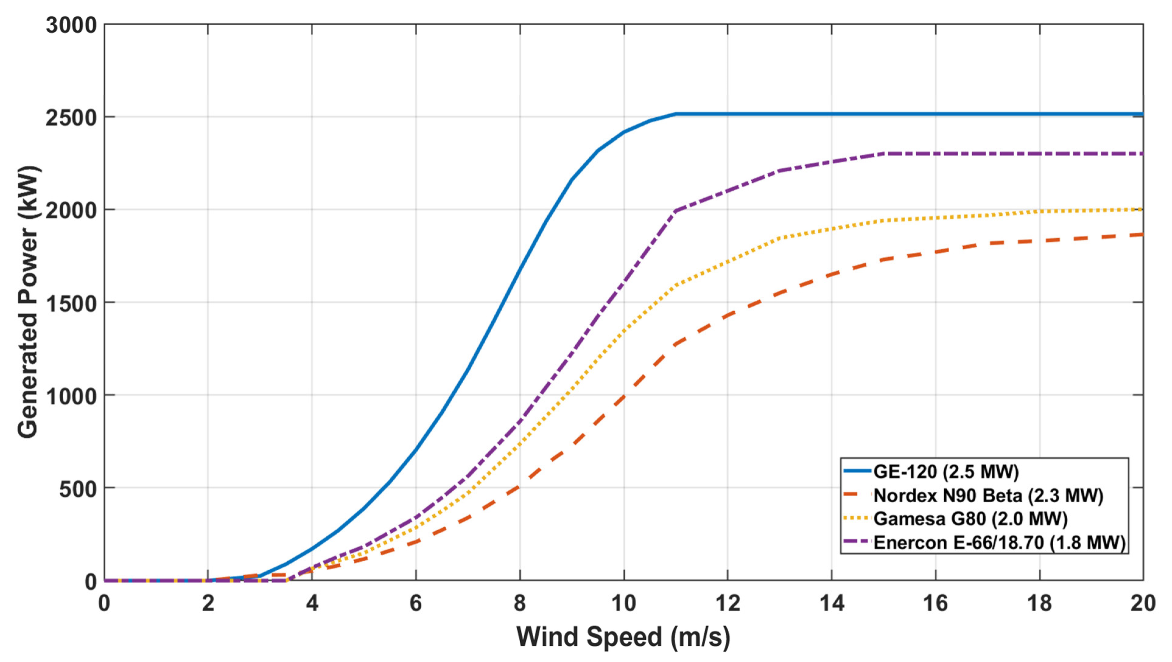
GE-120 (2.5 MW)	19	32	54	92
Nordex N90 Beta (2.3 MW)	19	30	54	85
Gamesa G80 (2.0 MW)	16	24	50	66
Enercon E-66/18.70(1.8 MW)	21	33	59	94

, the most suitable configuration can be established to harness the maximum wind power potential and maximize the capacity factor throughout the year. This information aids in making informed decisions regarding renewable energy investments and optimizing the utilization of wind resources in the respective power systems.

The use of the GWO algorithm in the optimization process yielded promising results. Specifically, the GWO algorithm facilitated the simultaneous mitigation of power loss and voltage deviation, while also optimizing wind placement. This successful implementation of the GWO algorithm contributed to the efficient integration of renewable energy sources into the power system, leading to enhanced system performance and increased utilization of renewable energy. Overall, these results demonstrated the potential of the GWO algorithm as a powerful tool for optimizing power system operation and promoting sustainable energy solutions. Further research is needed to investigate the applicability of the GWO algorithm to other power systems and to explore the potential for further improvements in renewable energy integration.

5.2.4. Site-Specific Wind Placement Sizing with Weibull Distribution Parameters

The Weibull distribution can be used for wind profile modeling in wind energy analysis. It provides a simple and practical approach to represent the frequency distribution of wind speeds at a specific location. By estimating the shape and scale parameters, the wind resource can be characterized. The probability density function definition of the Weibull distribution, as accepted in the literature, is given by Equation (19). As can be seen, it is defined in terms of two different variables: shape (k) and scale (c).

$$f\left(v;k,c\right)=\frac{k}{c}{\left(\frac{v}{ c}\right)}^{k-1}{e}^{-{\left(\frac{v}{ c}\right)}^k}$$

(19)

As seen in Figure 12, the histogram data in this study generated using the Weibull distribution were employed for wind simulation based on the scale and shape parameters c = 8.030 and k = 3.1571 (P1), and c = 10.0425 and k = 3.0966 (P2).

These data were evaluated in the model together with power profile data of four different contemporary wind turbine models given in Figure 13: GE 2.5 (MW)-120, Nordex N90 Beta (2.3 MW), Gamesa G80 (2 MW), and Enercon E-66/18.70 (1.8 MW). The simulation results included the analysis of optimization outcomes such as the maximum power value and capacity factor achievable in a year.

The calculated turbine quantities determined for Profile-1 (P1) and Profile-2 (P2), in order to meet the maximum connectable wind power of 9.8 MW for the IEEE 30-bus system used in P1, and that of 28.12 MW for the IEEE 118-bus system used in P2, revealed the optimal renewable investment opportunities based on the determined maximum power values.

6. Conclusions

In this study, the proposed GWO method aimed to address the ORPD problem by determining the optimal placement of wind energy in a power system. The optimization process focused on minimizing both the active power loss and voltage deviations, while ensuring that the control variables remained within their designated upper and lower bounds. This approach aimed to maximize the integration of renewable energy sources and minimize the associated losses.

To assess the performance of the proposed method, the authors utilized the IEEE 30-bus and IEEE 118-bus systems as case studies in their investigation. A comparison was conducted with other heuristic methods such as PSO, GA, ABC, OGSA, HBMO, and HFA in terms of various performance metrics including power loss minimization, voltage deviations, bus voltage levels, and number of iterations. The results obtained from the comparison highlighted the potential of the proposed GWO-based method for improving the performance and efficiency of power systems with increased renewable energy penetration. The reduced number of iterations needed for convergence is a notable advantage in terms of computational efficiency and practical implementation. These findings contribute to the understanding of the applicability and effectiveness of the GWO-based approach for addressing the ORPD problem and optimizing the placement of wind power to promote renewable energy integration.

In conclusion, the proposed GWO-based optimization method showed promising results in optimizing the placement of wind power to achieve optimal renewable penetration and dispatch. The comparisons with other methods and the evaluations of performance metrics supported the effectiveness and efficiency of the proposed approach. The results obtained from this study can provide valuable insights for researchers and practitioners in the field of power systems planning and operation, with the aim of promoting renewable energy integration in power systems.

References

- Zimmerman, R.D.; Murillo-Sánchez, C.E.; Thomas, R.J. MATPOWER: Steady-State Operations, Planning and Analysis Tools for Power Systems Research and Education. IEEE Trans. Power Syst. 2011, 26, 12–19. [Google Scholar] [CrossRef]
- Zhu, J. Optimization of Power System Operation; John Wiley Sons: Hoboken, NJ, USA, 2015. [Google Scholar] [CrossRef]
- Maskar, M.B.; Thorat, A.R.; Korachgaon, I. A review on optimal power flow problem and solution methodologies. In Proceedings of the International Conference on Data Management, Analytics and Innovation (ICDMAI), Pune, India, 24–26 February 2017; pp. 64–70. [Google Scholar] [CrossRef]
- Ting, C.-K. On the Mean Convergence Time of Multi-Parent Genetic Algorithms without Selection. In Advances in Artificial Life: 8th European Conference, ECAL 2005, Canterbury, UK, 5–9 September 2005; Springer: Berlin/Heidelberg, Germany, 2005; pp. 403–412. Available online: https://link.springer.com/chapter/10.1007/11553090_41 (accessed on 10 May 2023).
- Van Cutsem, T.; Vournas, C. Voltage Stability of Electric Power Systems; Springer: New York, NY, USA, 1998; Available online: https://link.springer.com/book/10.1007/978-0-387-75536-6 (accessed on 10 May 2023).
- Glavic, M.; Van Cutsem, T. Some Reflections on Model Predictive Control of Transmission Voltages. In Proceedings of the 38th North American Power Symposium (38th NAPS), Carbondale, IL, USA, 17–19 September 2006. [Google Scholar] [CrossRef]
- Carpentier, J. Contribution a l’etude du dispatching economique. Bull. Société Fr. Des Électriciens 1962, 8, 431–447. [Google Scholar]
- Carpentier, J. Optimal power flows. Int. J. Electr. Power Energy Syst. 1979, 1, 3–15. [Google Scholar] [CrossRef]
- Kou, X. Particle Swarm Optimization Based Reactive Power Dispatch for Power Networks with Distributed Generation. Master’s Thesis, University of Denver, Denver, CO, USA, 2015. Available online: https://digitalcommons.du.edu/etd/1035 (accessed on 10 May 2023).
- Norshahrani, M.; Mokhlis, H.; Abu Bakar, A.; Jamian, J.; Sukumar, S. Progress on Protection Strategies to Mitigate the Impact of Renewable Distributed Generation on Distribution Systems. Energies 2017, 11, 1864. [Google Scholar] [CrossRef]
- Al Rashidi, M.R.; El-Hawary, M.E. A Survey of Particle Swarm Optimization Applications in Electric Power Systems. IEEE Trans. Evol. Comput. 2009, 13, 913–918. [Google Scholar] [CrossRef]
- Salama, M.M.A.; Manojlovic, N.; Quintana, V.H.; Chikhani, A.Y. Real-Time Optimal Reactive Power Control for Distribution Networks. Electr. Power Energy Syst. 1996, 18, 185–193. [Google Scholar] [CrossRef]
- Shaw, B.; Mukherjee, V.; Ghoshal, S.P. Solution of reactive power dispatch of power systems by an opposition-based gravitational search algorithm. Int. J. Electr. Power Energy Syst. 2014, 55, 29–40. [Google Scholar] [CrossRef]
- Ghasemi, A.; Valipour, K.; Tohidi, A. Multi objective optimal reactive power dispatch using a new multi objective strategy. Electr. Power Energy Syst. 2014, 57, 318–334. [Google Scholar] [CrossRef]
- Rajan, A.; Malakar, T. Optimal reactive power dispatch using hybrid Nelder–Mead simplex based firefly algorithm. Int. J. Electr. Power Energy Syst. 2015, 66, 9–24. [Google Scholar] [CrossRef]
- Ghasemi, M.; Akbari, E.; Faraji Davoudkhani, I.; Rahimnejad, A.; Asadpoor, M.B.; Gadsden, S.A. Application of Coulomb’s and Franklin’s laws algorithm to solve large-scale optimal reactive power dispatch problems. Soft Comput. 2022, 26, 13899–13923. [Google Scholar] [CrossRef]
- Dutta, S.; Roy, P.K.; Manna, D.K. HBBO Optimization for Optimal Reactive Power Dispatch Incorporating TCSC and TCPS Devices. In Proceedings of the Michael Faraday IET International Summit, Kolkata, India, 12–13 September 2015; pp. 156–163. [Google Scholar] [CrossRef]
- Cao, Y.J.; Wu, Q.H. Optimal Reactive Power Dispatch Using an Adaptive Genetic Algorithm. In Proceedings of the Second International Conference on Genetic Algorithms in Engineering Systems, Glasgow, UK, 2–4 September 1997; pp. 117–122. [Google Scholar] [CrossRef]
- El-Ela, A.A.; Kinawy, A.M.; El-Sehiemy, R.A.; Mouwafi, M.T. Optimal reactive power dispatch using ant colony optimization algorithm. Electr. Eng. 2011, 93, 103–116. [Google Scholar] [CrossRef]
- Khanmiri, D.T.; Nasiri, N.; Abedinzadeh, T. Optimal Reactive Power Dispatch Using an Improved Genetic Algorithm. Int. J. Comput. Electr. Eng. 2012, 4, 463–472. [Google Scholar] [CrossRef]
- Esmin, A.A.; Lambert-Torres, G.; De Souza, A.Z. A hybrid particle swarm optimization applied to loss power minimization. IEEE Trans. Power Syst. 2005, 20, 859–866. [Google Scholar] [CrossRef]
- Sharif, S.S.; Taylor, J.H. Dynamic optimal reactive power flow. In Proceedings of the American Control Conference, Philadelphia, PA, USA, 26 June 1998; Volume 6, pp. 3410–3414. [Google Scholar] [CrossRef]
- Turkay, B.E.; Cabadag, R.I. Optimal Power Flow Solution Using Particle Swarm Optimization Algorithm. In Proceedings of the EUROCON, Zagreb, Croatia, 1–4 July 2013; pp. 1418–1424. [Google Scholar] [CrossRef]
- Om, H.; Shukla, S. Optimal Power Flow Analysis of IEEE-30 Bus System Using Soft Computing Techniques. Int. J. Eng. Res. Sci. (IJOER) 2015, 1, 55–60. [Google Scholar]
- Ayan, K.; Kılıç, U. Artificial Bee Colony Algorithm Solution for Optimal Reactive Power Flow. Appl. Soft Comput. 2012, 12, 1477–1482. [Google Scholar] [CrossRef]
- El-Shimy, M.; Abuel-wafa, A.R. Implementation and Analysis of Genetic Algorithms (GA) to the Optimal Power Flow (OPF) Problem. Sci. Bull. Fac. Eng. Ain Shams Univ. 2006, 41, 753–771. [Google Scholar] [CrossRef]
- Devaraj, D. Improved genetic algorithm for multi-objective reactive power dispatch problem. Eur. Trans. Electr. Power 2007, 17, 569–581. [Google Scholar] [CrossRef]
- Mamandur, K.R.C.; Chenoweth, R.D. Optimal Control of Reactive Power Flow for Improvements in Voltage Profiles and for Real Power Loss Minimization. IEEE Trans. Power Appar. Syst. 1981, 7, 3185–3194. [Google Scholar] [CrossRef]
- Kumar, C.; Raju, C.P. Constrained Optimal Power Flow Using Particle Swarm Optimization. Int. J. Emerg. Technol. Adv. Eng. 2012, 2, 235–241. [Google Scholar] [CrossRef]
- Dai, C.; Chen, W.; Zhu, Y.; Zhang, X. Seeker Optimization Algorithm for Optimal Reactive Power Dispatch. IEEE Trans. Power Syst. 2009, 24, 1218–1231. [Google Scholar] [CrossRef]
- Le Dinh, L.; Vo Ngoc, D.; Vasant, P. Artificial Bee Colony Algorithm for Solving Optimal Power Flow Problem. Sci. World J. 2013, 2013, 159040. [Google Scholar] [CrossRef]
- Mouassa, S.; Bouktir, T. Artificial Bee Colony Algorithm for Discrete Optimal Reactive Power Dispatch. In Proceedings of the International Conference in Industrial Engineering and Systems Management, Seville, Spain, 21–23 October 2015; pp. 654–662. [Google Scholar] [CrossRef]
- Ettappan, M.; Vimala, V.; Ramesh, S.; Kesavan, V.T. Optimal reactive power dispatch for real power loss minimization and voltage stability enhancement using Artificial Bee Colony Algorithm. Microprocess. Microsyst. 2020, 76, 103085. [Google Scholar] [CrossRef]
- Monti, A.; Ponci, F. Electric Power Systems. In Intelligent Monitoring, Control, and Security of Critical Infrastructure Systems; Springer: Berlin/Heidelberg, Germany, 2015; pp. 31–65. [Google Scholar] [CrossRef]
- Zhang, X.P. Electric Power System Analysis, Operation and Control. Electr. Eng. 2006, 3, 1–42. [Google Scholar] [CrossRef]
- Gautam, L.K.; Mishra, M.; Bisht, T. A Methodology for Power Flow & Voltage Stability Analysis. Int. Res. J. Eng. Technol. 2015, 2, 321–326. [Google Scholar]
- Ling, S.H.; Iu, H.H.; Chan, K.Y.; Lam, H.K.; Yeung, B.C.; Leung, F.H. Hybrid particle swarm optimization with wavelet mutation and its industrial applications. IEEE Trans. Syst. Man Cybern. Part B 2008, 38, 743–763. [Google Scholar] [CrossRef]
- Liu, Y.; Ćetenović, D.; Li, H.; Gryazina, E.; Terzija, V. Multi-objective optimization approaches have also been used in ORPD studies. Int. J. Electr. Power Energy Syst. 2022, 136, 107764. [Google Scholar] [CrossRef]
- Mouassa, S.; Bouktir, T. Multi-objective ant lion optimization algorithm to solve large-scale multi-objective optimal reactive power dispatch problem. COMPEL-Int. J. Comput. Math. Electr. Electron. Eng. 2019, 38, 304–324. [Google Scholar] [CrossRef]
- Beyer, H.-G. The Theory of Evolution Strategies; Springer Science & Business Media: Berlin/Heidelberg, Germany, 1995. [Google Scholar] [CrossRef]
- Hansen, N.; Ostermeier, A. Completely derandomized self-adaptation in evolution strategies. Evol. Comput. 2001, 9, 159–195. [Google Scholar] [CrossRef]
- Sulaiman, M.H.; Mustafa, M.W.; Aliman, O.; Khalid, S.A.; Shareef, H. Real and reactive power flow allocation in deregulated power system utilizing genetic-support vector machine technique. Int. Rev. Electr. Eng. 2010, 5, 2199–2208. [Google Scholar]
- Mustafa, M.W.; Sulaiman, M.H.; Shareef, H.; Khalid, S.A. Reactive power tracing in pool-based power system utilising the hybrid genetic algorithm and least squares support vector machine. IET Gener. Transm. Distrib. 2012, 6, 133–141. [Google Scholar] [CrossRef]
- Jarmouni, E.; Mouhsen, A.; Lamhammedi, M.; Ouldzira, H. Integration of artificial neural networks for multi-source energy management in a smart grid. Int. J. Power Electron. Drive Syst. 2021, 12, 1919. [Google Scholar] [CrossRef]
- Lateef, A.A.A.; Ali Al-Janabi, S.I.; Abdulteef, O.A. Artificial Intelligence Techniques Applied on Renewable Energy Systems: A Review. In Proceedings of International Conference on Computing and Communication Networks: ICCCN; Springer: Singapore, 2021; pp. 297–308. [Google Scholar] [CrossRef]
- DingPing, L.; GuoLiang, S.; WenDong, G.; ZHi, Z.; BaoNing, H.; Wei, G. Power system reactive power optimization based on MIPSO. Energy Procedia 2012, 14, 788–793. [Google Scholar] [CrossRef]
- Yang, T.; Zhao, L.; Li, W.; Zomaya, A.Y. Reinforcement learning in sustainable energy and electric systems: A Survey. Annu. Rev. Control. 2020, 49, 145–163. [Google Scholar] [CrossRef]
- Mirjalili, S.; Mirjalili, S.M.; Lewis, A. Grey wolf optimizer. Adv. Eng. Softw. 2014, 69, 46–61. [Google Scholar] [CrossRef]
- Abbas, M.; Alshehri, M.A.; Barnawi, A.B. Potential Contribution of the Grey Wolf Optimization Algorithm in Reducing Active Power Losses in Electrical Power Systems. Appl. Sci. 2022, 12, 6177. [Google Scholar] [CrossRef]
- Mohseni-Bonab, S.M.; Rabiee, A.; Mohammadi-Ivatloo, B.; Jalilzadeh, S.; Nojavan, S. A two-point estimate method for uncertainty modeling in multi-objective optimal reactive power dispatch problem. Int. J. Electr. Power Energy Syst. 2016, 75, 194–204. [Google Scholar] [CrossRef]
- Shaheen, M.A.; Yousri, D.; Fathy, A.; Hasanien, H.M.; Alkuhayli, A.; Muyeen, S.M. A novel application of improved marine predators algorithm and particle swarm optimization for solving the ORPD problem. Energies 2020, 13, 5679. [Google Scholar] [CrossRef]
- Electric Power Group. “Transmission System Planning Reference Book”, 118-Bus Test System. 2004. Available online: https://www.electricitypolicy.org.uk/pdfs/wp8.pdf. (accessed on 21 April 2023).
- Sulaiman, M.H.; Mustaffa, Z.; Mohamed, M.R.; Aliman, O. Using the gray wolf optimizer for solving optimal reactive power dispatch problem. Appl. Soft Comput. 2015, 32, 286–292. [Google Scholar] [CrossRef]