Techno-Economic Analysis and Optimization of a Compressed-Air Energy Storage System Integrated with a Natural Gas Combined-Cycle Plant

Abstract

To address the rising electricity demand and greenhouse gas concentration in the environment, considerable effort is being carried out across the globe on installing and operating renewable energy sources. However, the renewable energy production is affected by diurnal and seasonal variability. To ensure that the electric grid remains reliable and resilient even for the high penetration of renewables into the grid, various types of energy storage systems are being investigated. In this paper, a compressed-air energy storage (CAES) system integrated with a natural gas combined-cycle (NGCC) power plant is investigated where air is extracted from the gas turbine compressor or injected back into the gas turbine combustor when it is optimal to do so. First-principles dynamic models of the NGCC plant and CAES are developed along with the development of an economic model. The dynamic optimization of the integrated system is undertaken in the Python/Pyomo platform for maximizing the net present value (NPV). NPV optimization is undertaken for 14 regions/cases considering year-long locational marginal price (LMP) data with a 1 h interval. Design variables such as the storage capacity and storage pressure, as well as the operating variables such as the power plant load, air injection rate, and air extraction rate, are optimized. Results show that the integrated CAES system has a higher NPV than the NGCC-only system for all 14 regions, thus indicating the potential deployment of the integrated system under the assumption of the availability of caverns in close proximity to the NGCC plant. The levelized cost of storage is found to be in the range of 136–145 $/MWh. Roundtrip efficiency is found to be between 74.6–82.5%. A sensitivity study with respect to LMP shows that the LMP profile has a significant impact on the extent of air injection/extraction while capital expenditure reduction has a negligible effect.

1. Introduction

Global electricity generation is expected to increase by 150% by 2050 [1]. A large share of this increase is expected to be generated from non-fossil energy sources due to efforts all over the world on curtailing greenhouse gas emissions. In many countries, a large portion of the existing fossil-based power generation sources is expected to be replaced by renewable energy sources. However, these renewable energy sources such as solar and wind energy are intermittent with a large variation in their generation capabilities. In addition, wind and solar energy both can be strongly affected by diurnal and seasonal variabilities, along with considerable variation from one region to another. It is also desired that future electricity generation sources can reliably address variabilities in demand. Lack of capabilities to address the variabilities in the demand and supply of electricity can cause major issues with grid reliability and resiliency and can eventually restrict the extent of penetration of renewables to the grid. One potential approach to address these issues is to consider energy storage. Based on the maximum discharge time at the rated power, energy storage systems (ESSs) are generally classified as: short-term (seconds to minutes), such as the super capacitors, flywheel, etc.; mid-term (minutes to several hours), such as batteries, i.e., Li-ion battery, various types of flow batteries, NaS battery, etc.; and long-term (hours to several days), such as the compressed-air energy storage (CAES) and pumped-hydro energy storage [2], as well as hydrogen storage. The selection of the appropriate ESS strongly depends on the intended application and other critical parameters. The selection criteria for the optimal storage technology in a specific region depend on various storage properties such as energy density, output density, storage efficiency and capacity, charging and discharging times, transient response, partial load capability, lifetime, reliability, safety, location, and construction time, among others [3].

In addition to ESSs that are very suitable for peak-shaving or load-leveling applications [4], it is desired to investigate ESSs that are suitable for long-term energy storage including seasonal storage. Some of the long-term storage options such as pumped hydro and CAES can benefit from cheap large storage volumes if natural formations are available [5]. There are considerable variabilities in the availability and accessibility of such natural formations from region to region. Pumped hydro can have an adverse environmental impact on the local flora and fauna [6,7]. Another potential energy storage technology for long-term storage is the hydrogen storage system; however, the economic viability, scalability, and safety of hydrogen storage are still being investigated, restricting them to mainly small-scale storage applications. In contrast, CAES has a long history of successful operation. For example, the 290 MWe Huntorf plant in Germany has been operating since 1978 [1] and the 110 MWe plant in McIntosh, USA has been operating since 1991 [2]. These plants have been utilized in evaluating the capability of CAES for peak shaving, load following, load shifting, and regulation [7]. Additional CAES are under construction or have been recently commissioned [8,9]. Furthermore, CAES has various options for storage such as underground salt domes, natural formation such as aquifers, abandoned oil wells, aboveground storage vessels, etc., thus making them feasible in many regions.

CAES can be used along with thermal and nuclear power plants [7,10,11] for mid- to long-term energy storage, enabling the load-following operation of those power plants without deviating much from their design base-loaded operation. CAES can be integrated with wind energy systems for obtaining high-rated power and high energy capacity, leading to a lower levelized cost of storage (LCOS). In general, off-peak cheap electricity can be used to compress air and store it. This pressurized air is sent through expanders to generate electricity during high demand. Existing commercial CAES systems store air in underground caverns since caverns are far more cost-effective compared to above-ground pressure vessels [7,8].

The optimal selection and design of long-term CAES are expected to vary greatly from region to region based on various factors but most prominently on the demand and supply profile of electricity and seasonal variability. Furthermore, these storage systems can be placed as a standalone facility and/or integrated with fossil-fueled power plants (FFPPs). In the latter case, existing assets in FFPPs can be utilized, thus reducing the capital costs. While there are several publications on the modeling of CAES based on different configurations and power plant application [7,12,13,14,15,16,17], those studies mainly consider the independent operation of the CAES and FFPPs. There are few works in the existing literature that have investigated the design and operation of these storage systems integrated with FFPPs. Jeong et al. [18] have considered mass and thermal integration between CAES and a natural gas combined-cycle (NGCC) plant. For thermal integration, the high-pressure air from the cavern is heated by a portion of the exhaust stream from the gas turbine (GT) in the NGCC plant and the exhaust from the low-pressure turbine is injected into the heat recovery steam generator (HRSG). Since air from CAES is extracted at the time of high electricity demand and/or high electricity price, such thermal integration makes the control and operation of the integrated system challenging. Jeong et al. [18] have considered only mass integration, in which a portion of the air is extracted from the high-pressure expander in the CAES system and injected into the GT combustor of the NGCC plant. However, there are two modifications to the mass integration scheme of Jeong et al. [18] that can possibly save capital cost and perhaps operating costs. First, the entire amount of air from the high-pressure expander can be sent to the GT combustor in the NGCC plant. This modification can eliminate the cost of a separate combustor and a low-pressure expander in the CAES system. This modification can also benefit from the highly efficient, large-scale NGCC GT combustor and expander. Second, it may be possible to extract a portion of the air from the exhaust or from intermediate stages of the GT compressor in the NGCC plant and then compress it further, as needed, before sending it to storage. It should be noted that air is routinely extracted from the GT compressor in the industry [19]. Igie et al. [20] have suggested that the extraction of air after the last stage is appropriate for large flows of up to about 15% of the compressor inlet flow. Wojcik and Wang [21] have investigated air extraction from the GT compressor at various GT loads. The maximum extent of air extraction from a GT compressor stage depends on the machine type and can be enhanced through modifications to casings, piping, and controls. Nevertheless, this modification can reduce the size of the low-pressure compressor in the CAES system or can completely eliminate it, thus saving capital cost. This modification can also benefit from the highly efficient GT compressor.

Techno-economic analysis of the integrated CAES system is scarce. Kruk-Gotzman et al. [22] have investigated the thermal integration of the CAES and NGCC. Salvini [23] has evaluated the thermal integration of HRSGs integrated with the CAES. He et al. [24] have studied the thermodynamics of CAES with NGCC and have proposed to use the compression heat from the CAES system for the cracking reaction of methanol, thus avoiding thermal energy storage.

To the best of our knowledge, there is no work in the current open literature focused on the optimal design and operation of the CAES integrated with the NGCC plant by considering the optimal operation of the integrated system due to the varying demand and supply profile and/or varying locational marginal price (LMP) of electricity. For the optimal design of the integrated CAES system, it is desired to consider the long-term demand/supply profile and/or LMP. In particular, when long-term storage is considered, the demand/supply profile and/or LMP for at least one year is desired, if not more, to take into consideration seasonal variabilities along with diurnal variabilities. Variabilities in demand/supply/LMP can be obtained from the historical data [25] or forecast.

For optimizing the design and operation of the integrated CAES system, it is also necessary to simultaneously optimize the operation of the NGCC plant irrespective of whether the CAES is retrofitted to an existing NGCC plant or integrated with a grassroots NGCC plant. However, since the dynamics of the CAES and NGCC plant should be considered for the optimization, if a long-term optimization (such as 1 year or more) is undertaken with a fine time resolution (such as second/minute/hour), a large-scale dynamic optimization problem needs to be solved. For example, if a fully discretized approach to dynamic optimization is used and if there are just 1000 model equations for the integrated system, then considering a time resolution of 1 h and 8000 h of operation in a year, it will lead to 8 MM equality constraints. Obviously, there would be a large number of decision variables. A suitable optimization approach including model simplification and reformulation, if needed, should be devised for effectively solving this large-scale dynamic optimization problem. Most of the optimization studies in the literature deals with the integration of CAES with a photovoltaic power plant [26,27], wind power [28,29,30,31], and thermal energy storage system [32,33], where the number of model equations is relatively low. For computational tractability of the optimization problem, some of the common approaches are to consider just a single day or a few days as the representative days for the year, make steady-state assumptions for all units except the storage vessel itself, use linear models and reduced order models, as well as use varieties of optimization algorithms for nonlinear programming (NLP) [26] and deterministic dynamic programing (DP), in addition to convex optimization [28], mixed integer nonlinear programing (MINLP) with piece-wise linearization and the auxiliary binary variable method [31], parametric analysis and structure optimization [32], mixed integer co-optimization [34], or heuristic optimization algorithms such as the genetic algorithm [35].

In summary, there is no study found in the current open literature that has undertaken a large-scale dynamic optimization of the integrated CAES system. In addition, our literature review shows that there is no study that has undertaken a net present value (NPV) optimization of the integrated CAES system using year-long LMP data—this is one of the key gaps in the existing literature that this paper seeks to fill in. Furthermore, the configuration of the integrated system that this paper considers eliminates the need for a separate low-pressure compressor, combustor, and low-pressure expander in the CAES, by utilizing the existing assets of the NGCC plant. In addition, since the optimal design and operation of the integrated CAES can vary depending on variabilities in LMP, the impact of LMP for 14 regions (some of these can be called cases or scenarios, but for convenience, we refer to them as regions) is studied. This study seeks to answer the following questions:

• What are the optimal design of CAES and operating conditions of the CAES and NGCC plant for a given LMP profile?
• Which region is favorable (i.e., has a positive NPV) for the integrated CAES and how do the optimal design and operation of the integrated CAES system differ from region to region?
• Which cost components have a high impact on NPV and what extent of reduction in a cost component can make the integrated CAES system favorable in an otherwise unfavorable region?

This article is organized as follows: Section 2 presents the models of the NGCC plant and CAES and their validation, and the reduced order model development for the NGCC plant. Section 3 presents the optimization formulation and solution approach. Section 4 discusses the optimization results for different regions that differ widely in terms of LMP profile and several sensitivity studies. Finally, Section 5 highlights the key findings of the work.

2. Model Development and Validation

2.1. NGCC Model Development

An NGCC plant with a gross power output of 641 MWe is considered for integration with the CAES technology. A nonlinear high-fidelity dynamic model of the NGCC plant was developed in Aspen Plus Dynamics (APD) based on the process configuration and design conditions given in the B31A baseline study conducted by the U.S. Department of Energy’s National Energy Technology Laboratory (NETL) [36]. The NGCC model consists of three main sections—the GT section, heat recovery steam generator (HRSG) section, and steam turbine (ST) section. The GT is modeled by using dimensionless performance curves for head and isentropic efficiency versus volumetric flowrate. The HRSG section produces steam at three pressure levels—high pressure (HP), medium pressure (MP), and low pressure (LP)—by using several heat exchanger sections that are modeled by using the $ϵ$-NTU method. The ST model has an impulse type of governing stage, and mixed impulse–reaction stages for other stages, with capabilities for detecting moisture and accounting for that, if moisture is present, not only for the last stage but intermediate-stage models as well. Regulatory and supervisory control layers similar to the industry-standard co-ordinated control systems are designed and implemented for the plant-wide system. For more details on the design, model, and simulation of the NGCC plant, interested readers are referred to the previous research articles published by one of the co-authors [10,11].

The NGCC model described in our earlier work [10,11] is modified by adding air injection and extraction streams. One important consideration for the GT model is to ensure that the turbine inlet temperature (TIT) is maintained during air injection from the CAES. During normal operation, the TIT is maintained by the GT control system at a given setpoint, which may change with the load, by manipulating the air/fuel ratio. As the temperature of the injected air can differ than the air compressed by the GT compressor, the air/fuel ratio for air injection, especially for a high air injection rate, can differ compared to the typical operation in the absence of any injection.

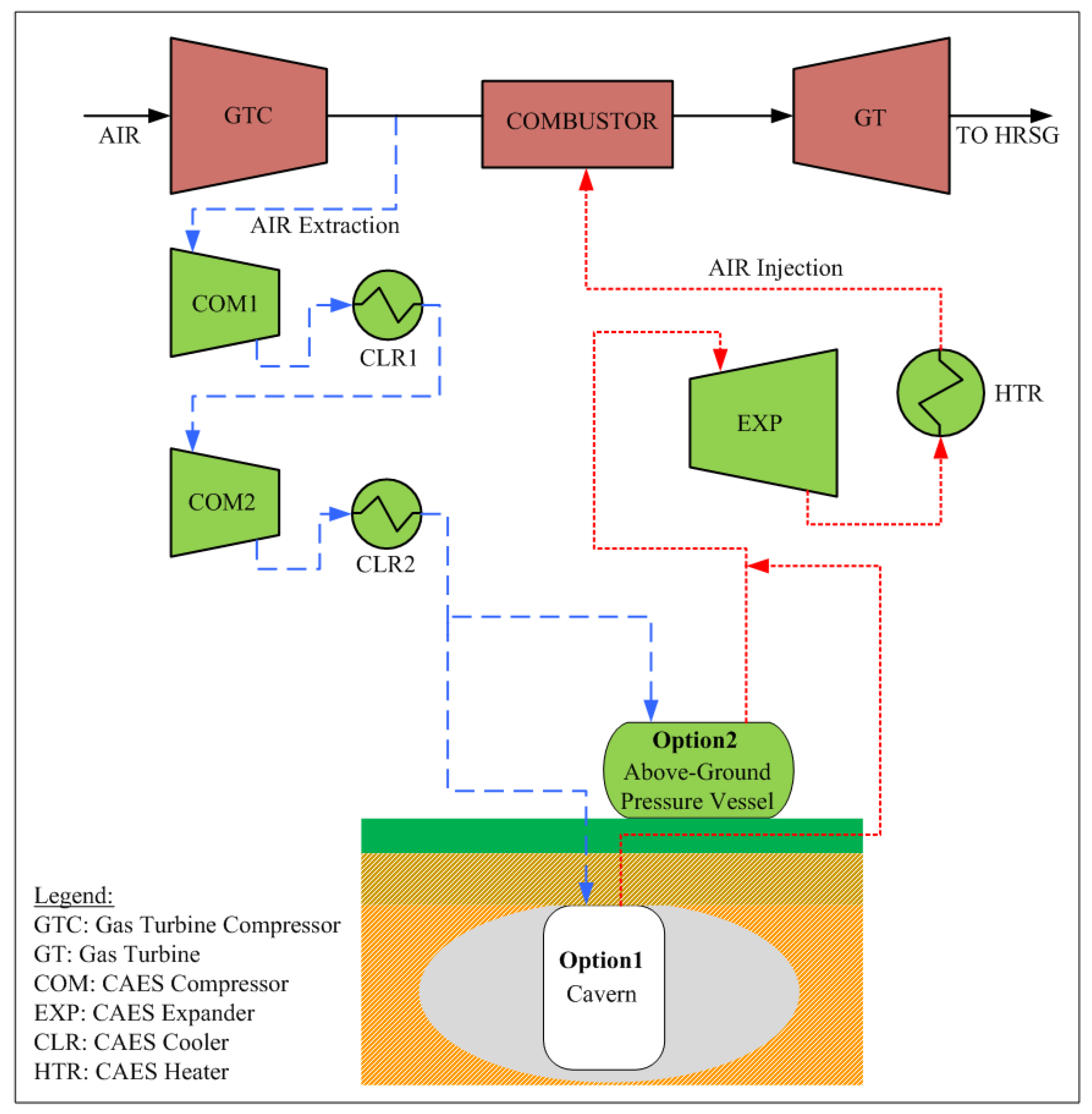
2.2. CAES Model Development

Figure 1 shows the configuration of the CAES system integrated with the NGCC plant. The CAES model has three sections—charging, storage, and discharging. The charging section comprises the compressor with an intercooler, while the discharging section has an expander and a heater. Air is extracted from the NGCC plant which is compressed by the multi-stage compressor with an intercooler before it is stored in the storage.

A nonisothermal dynamic model of the CAES is developed. The assumptions are as follows:

i.

Air is assumed to be an ideal gas. Given the pressure and temperature ranges of operation considered in this study (40–72 bar and 10–50 °C), the compressibility factor of air does not deviate much from 1.

ii.

The cavern is considered to be a well-mixed system and it is assumed to lose heat only through its wall. No other heat loss from the air is considered under the assumption that the incoming and existing air ducts are well-insulated.

The first-principles mathematical model of the cavern CAES storage is presented in

Table 1. Dynamic model equations of the CAES storage [7].

$\frac{d{\rho }_{air,st}}{dt}=\frac{{\dot{m}}_{in}-{\dot{m}}_{out}}{V_{cav}}$	(1)
$\frac{d\left(m\widehat{U}\right)}{dt}={\dot{m}}_{in}{\widehat{H}}_{in}-{\dot{m}}_{out}{\widehat{H}}_{out}-h_{eff}{A}_{cav}\left(T_{st}-T_{wall}\right)$	(2)
$\frac{d{T}_{st}}{dt}=\frac{\frac{{\dot{m}}_{in}-{\dot{m}}_{out}}{V_{cav}}\left(\frac{R{T}_{st}}{Mw}\right)-\frac{{\dot{m}}_{in}C{p}_{air}\left(T_{st}-T_{in}\right)}{V_{cav}}-\frac{h_{eff}{A}_{cavern}\left(T_{st}-T_{wall}\right)}{V_{cav}}}{{\rho }_{air,st}\left(C{p}_{air}-\frac{R_g}{Mw}\right)}$	(3)
$P_{air,st}=\frac{{\rho }_{air,st}{R}_g{T}_{st}}{Mw}$	(4)
$h_{eff}=0.2356+0.0149 {\left|{\dot{m}}_{in}-{\dot{m}}_{out}\right|}^{0.8}$	(5)

. Equations (1) and (2) represent the mass and energy balances of air in the storage, respectively. As the air is assumed to be an ideal gas and there is no phase change of air, Equation (2) leads to Equation (3). Equation (4) is used to calculate the pressure. Equation (5) is used to calculate the effective heat transfer coefficient.

Model equations for the expander/compressors and the heat exchangers are listed in

Table 2. Steady-state model equations of CAES system [31].

Compressor
$P_{c,i}=\frac{k{Q}_{m,c}{R}_g{T}_{c,i}^{in}}{\left(k-1\right) {\eta }_{c,i}}(({\beta }_{c,i}{)}^{\frac{k-1}{k}}-1)$	(6)
$T_{c,i}^{out}=T_{c,i}^{in}\left[\frac{{({\beta }_{c,i})}^{\frac{k-1}{k}}-1}{{\eta }_{c,i}}+1\right]$	(7)
$, \mathrm{where} {\beta }_{c,i}=\frac{P_{c,i}^{out}}{P_{c,i}^{in}}$
Cooler: Hot Fluid—Air, Cold Fluid—Water
$Q_m=m_{h}C{p}_h\left(T_{h,in}-T_{h,out}\right)$	(8)
$Q_{cw}=m_{cw}C{p}_{cw}\left(T_{cw,out}-T_{cw,in}\right)$	(9)
Heat transfer area calculation
$Q=UA\Delta T_{lmtd}$	(10)
$, \mathrm{where} \Delta T_{lmtd}=\frac{\left(T_{h,in}-T_{cw,out}\right)-\left(T_{h,out}-T_{cw,in}\right)}{ln\left(\frac{T_{h,in}-T_{cw,out}}{T_{h,out}-T_{cw,in}}\right)}$

[31]. Equations (6) and (7) are used to compute the power requirement and discharge temperature for a single compression stage. Similar equations are written for the expander. Equations (8)–(10) are used to model the cooler. The compressed air from the outlet of each compressor is sent to the cooler where water is used as the cold utility. A similar equation is used for the heater, but LP steam is used for the hot utility, so the equations are modified accordingly. It should be noted that heat recovery is not considered here, as cooling (needed during charging) and heating (needed during discharging) will not occur at the same time. Furthermore, as the optimal air extraction and injection will vary with LMP, i.e., the compression and expansion equipment will run at different flowrates at different instants of time, heat integration for this system is difficult. One possible option is to consider an external thermal storage, which is not considered in this work.

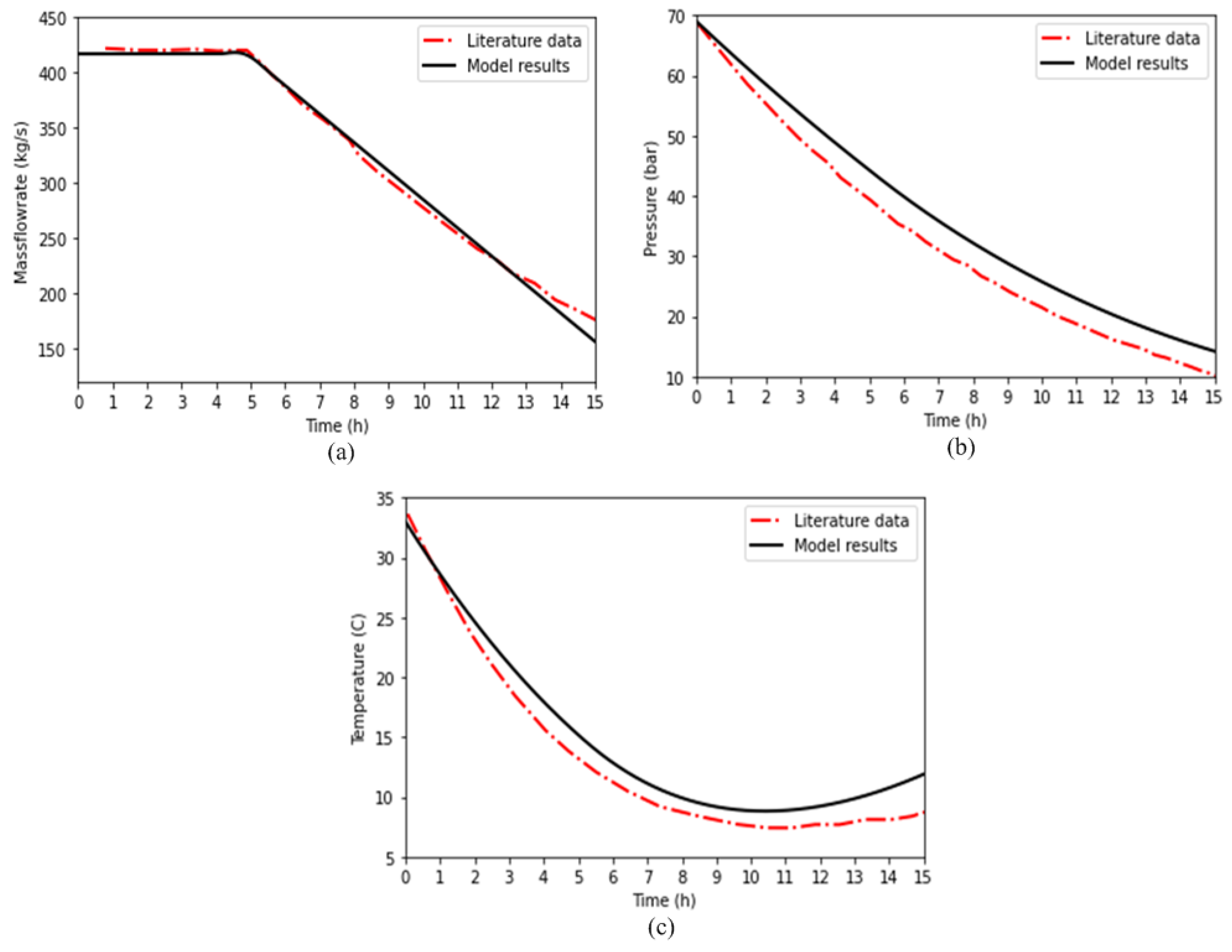
2.3. CAES Model Validation

The dynamic pressure and temperature profiles inside the cavern are compared with that for the data from the Huntorf plant in Germany [7,37,38]. The corresponding initial and operating conditions are presented in

Table 3. Design and operating conditions of Huntorf plant [7].

Description	Value
Design & Operating Conditions
Inlet temperature (Tin), K	330
Mass flowrate ($m_{in}$), kg/s	417
Volume of the cavern (m3) Ambient temperature (Twall), K	3,000,000 330
Initial Conditions (discharge cycle)
Air storage density, kg/m3	76.24
Mass flowrate, kg/s	417
Pressure, bar	69
Temperature, °C	33

[7]. A constant discharge rate of 417 kg/s is considered till the fifth hour, and then the discharge mass flow rate decreases till 15 h. The mass flowrate to the storage, resulting pressure and temperature dynamics, and their comparison with the plant data are shown in Figure 2a–c, respectively. The developed model shows a close match with the plant data. RMSE between the data and model results for the pressure and temperature are approximately 4.92 bar and 1.88 °C, respectively. Figure 2c shows that the temperature decreases to a minimum (about 8.8 °C) around the 10th hour before it slowly starts rising due to heat transfer between the cavern wall and air, lower discharge rate, and increasingly smaller mass of air in the storage.

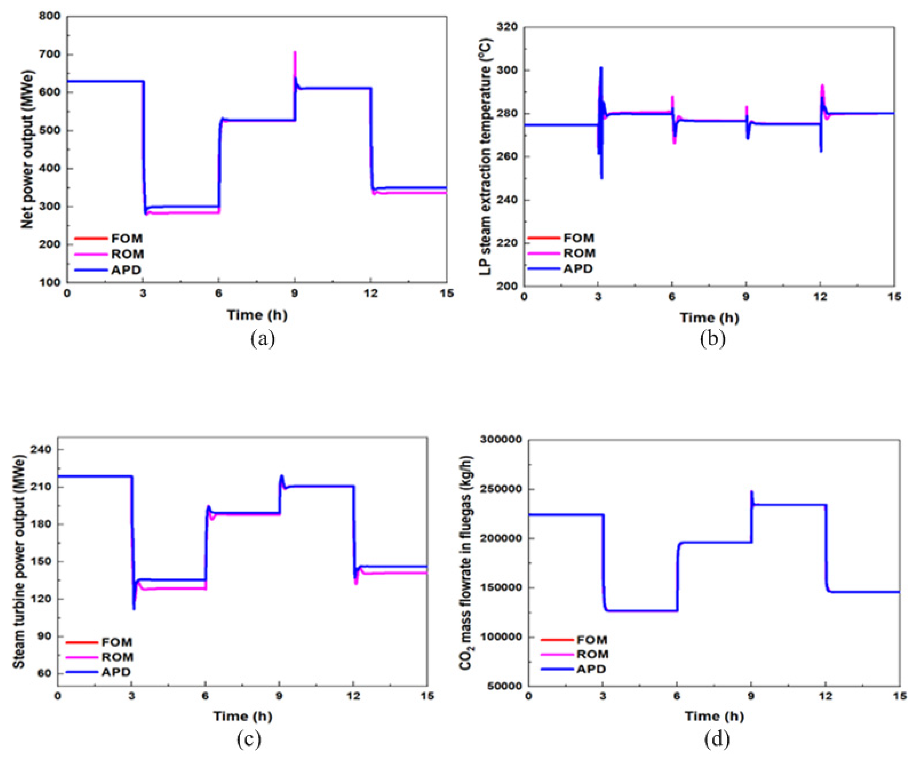
2.4. Reduced Order Model (ROM) Development

2.4.1. ROM Development for the NGCC Plant Integrated with Compressed Air Extraction/Injection

The nonlinear APD model of the NGCC plant with air extraction and injection described in Section 2.1 comprises more than a hundred thousand equations [10,11]. The model is computationally expensive for use in optimization, especially for dynamic optimization. Linear ROMs are considerably more suitable for a faster execution.

The nonlinear APD model described in Section 2.1 is given, in its generic form, by:

$$\dot{ x}=f\left(x\left(t\right),u\left(t\right)\right)$$

(11)

$$y=g\left(x\left(t\right),u\left(t\right)\right);x\left(t\right)\in R , u\in U$$

(12)

The continuous-time state-space model can be developed by linearizing the nonlinear model around the full/part-load condition:

$$\dot{x}=Ax\left(t\right)+Bu\left(t\right)$$

(13)

$$y=Cx\left(t\right)+Du\left(t\right)$$

(14)

This model is denoted as full-order model (FOM) as the size of the model matches the number of differential state variable in the APD model. This model is still large for use in optimization. Therefore, an ROM is developed through balanced truncation by using Hankel singular values. This method helps to preserve the stability of the model and can still reduce the global error bound [11,39]. The form of this model is given by:

$$\dot{x_{ROM}}=A_{ROM}x\left(t\right)+B_{ROM}u\left(t\right)$$

(15)

$$y=C_{ROM}x\left(t\right)+D_{ROM}u\left(t\right)$$

(16)

2.4.2. Linear MIMO State-Space Model for NGCC Plant Integrated with Air Extraction/Injection

The APD model has several hundred inputs and thousands of outputs, but only a few of them are needed for NPV optimization. For developing the state-space model to be used in NPV optimization, inputs that are considered are those that are optimization variables or boundary variables of the NGCC plant affected by the operation of the CAES while outputs of interest are those that are used for computing the NPV, or used as constraints in the optimization or used as input for the CO₂ capture unit. In particular, the following inputs are considered—natural gas flowrate (kg/h), GT air extraction flowrate (kg/h), GT air injection flowrate (kg/h), and GT air injection temperature (°C)—and the outputs are net power output (MWe), ST power output (MWe), CO₂ mass flowrate in flue gas (kg/h), and LP steam extraction temperature (°C). Input variables are dynamically varied and tested for the analysis of the ROM model. Figure 3a–d show the dynamic variation of the input variables—natural gas flowrate, GT air extraction flowrate, GT air injection flowrate, and GT air injection temperature, respectively, and

Table 4. Variation considered in the GT air extraction and injection flowrate.

Parameter	Extraction Sites	Injection Sites
GT-Air Compressor (Discharge site)	Extraction flowrate range: 50–86,000 kg/h	Injection flowrate range: 50–72,000 kg/h Injection temperature range: 424.5–530 °C

shows the range of GT air extraction/injection flowrate considered in this study.

Output responses from the nonlinear high-fidelity APD model, the full-ordered state-space model (FOM), and ROM are compared and shown in Figure 4. It can be observed that the results obtained from the ROM are satisfactory for all the outputs that are compared. For all the cases, both the FOM and ROM show almost the same responses and, therefore, the transient responses of FOM and ROM are not distinguishable in Figure 4. The linear ROM at full load shows excellent accuracy with respect to the high-fidelity nonlinear model in APD but the discrepancy at low-load conditions is higher and, considering all output variables of interest for NPV optimization at all time instants, the maximum instantaneous error is found to be about 6%. The discrepancy under low-load conditions could be addressed through the development of ROM by linearizing around lower-load conditions. However, such ROMs were found to result in higher inaccuracy at high-load conditions. One possible option for achieving high accuracy over the entire load range is to consider a bank of linear models. However, this would lead to difficulty in the large-scale dynamic NPV optimization due to possible discontinuities between models and disjunctions, and was therefore not considered.

3. Process Optimization

3.1. NPV Optimization Formulation

Equation (17) shows the main objective for the techno-economic analysis, which is to maximize the NPV of the integrated system by optimizing the parameters of the system such as the amount of power sold, the CAPEX and OPEX, and the penalty due to carbon emissions from the system. The interest rate is set at 7.25% and the corporate tax is fixed at 21%. The plant lifetime is considered to be 30 years. The main contributor to the revenue is the net power sold to the grid. Revenue calculations are given by Equation (18). It includes the net power sales to the grid, fuel cost mainly due to the cost of natural gas fed to the GT, carbon tax for CO₂ emission, and fixed and variable OPEX from all the units in the integrated plant including startup costs. The net power being sold to the grid at any time instant, given by ${\mathrm{P}}_{\mathrm{grid},\mathrm{t}}$, is calculated using Equation (20), where ${\mathrm{P}}_{\mathrm{gross},\mathrm{t}}$ denotes gross power being generated by the NGCC GT and ST, ${\mathrm{P}}_{\mathrm{gen},\mathrm{t}}$ denotes additional power generated by the expander in CAES, and ${\mathrm{P}}_{\mathrm{cons},\mathrm{t}}$ denotes additional power consumed by all equipment items in the NGCC–CAES system including CAES compressors. To simplify the problem, all utility duty is converted to the electrical equivalent and included in the computation of power consumption, $P_{cons,t}$, in Equation (20). The electrical equivalent for the LP steam used for heating is calculated based on the results from the LP turbine section in the NGCC model. THE Electrical equivalent for cooling is calculated based on the open literature [40]. The NPV optimization is formulated for the NGCC-only case and NGCC plant integrated with CAES case. Both cases are considered with the possibility of shutdown, i.e., the plant can shut down if that is optimal (e.g., when LMP is low).

$$\max NPV=P_{A,f} \left(1-tax\right){\displaystyle \sum }_{t=1}^{8760}REVENU{E}_t-CAPE{X}_{total}\left(1-\frac{tax}{n}{P}_{A,f}\right)$$

(17)

$$REVENU{E}_t=LM{P}_t·P_{grid,t}-C_{NG}·N{G}_t-C_{C{O}_2}·C{O}_{2,released}-OPE{X}_{variable}-OPE{X}_{fixed}$$

(18)

$$P_{A,f}=\frac{{\left(1+i\right)}^n-1}{i{\left(1+i\right)}^n}$$

(19)

$$P_{grid,t}=P_{gross,t}-P_{cons,t}+P_{gen,t}$$

(20)

The integrated NGCC–CAES system is considered to be an isolated system; thereby, there is no transfer of energy from/to other external units. The plant can only provide power to the grid, but cannot consume power from the grid (i.e., the integrated system cannot consume more power than it generates), and this is established by using the inequality constraint given by Equation (21) for the net power to the grid $P_{grid,t}$. In this work, no constraint from the perspective of grid demand is considered, as only a single NGCC plant is considered. Therefore, no upper bound is considered for $P_{grid,t}$. Constraints given by Equations (22) and (23) ensure that the plant gross power production and natural gas consumption remain bounded between values corresponding to 25% to 100% load. To keep the plant as an independent system on a year-to-year basis, the initial air storage density is used as a decision variable which is then constrained to be the same as that at the end of the year to ensure that the net change in the inventory over the entire year remains zero—this constraint is given by Equation (24). Moreover, since air extraction, air injection, and idling should be mutually exclusive at any given time instant, Equation (25) is used as a constraint, where ${ϵ}_{small}$ is a small positive number. There is a constraint on the maximum air extraction and injection for an existing gas turbine installation which is 15% of the total air flow in kg/h [20], and this is implemented by using Equation (26). Two additional constraints given by Equations (27) and (28) are added to constrain the storage volume and pressure.

$$P_{grid,t}\ge 0$$

(21)

$$P_{gross,25}\le P_{gross,t}\le P_{gross,100}$$

(22)

$$N{G}_{25}\le N{G}_t\le N{G}_{100}$$

(23)

$${\rho }_{Air,initial}={\rho }_{Air,final}$$

(24)

$$F_{extraction,t}·F_{injection,t}\le {ϵ}_{small}$$

(25)

$$0\le Air Flow \le 543,564$$

(26)

$$0<V_{storage}<3,000,000$$

(27)

$$40<P_{pr,storage}<72$$

(28)

LCOS is calculated by using Equation (29), where $F_A$ denotes the factor for annuitizing the capital cost, $CAPE{X}_{CAES}$ denotes the capital cost of the cavern and all equipment items in CAES, $OPE{X}_{CAES}$ denotes the fixed OPEX of CAES, $OPE{X}_{var,CAES}$ denotes the variable non-fuel operating costs of CAES (such as the cooling tower chemical and water makeup, etc.), $∆P_{prod, CAES,t}$ denotes the power produced by the CAES expander and the incremental power produced by the NGCC plant, $OPE{X}_{var,NGCC,t}$ denotes the variable cost of the NGCC plant including the fuel and utilities costs (as the CAES is driven by using the power from the NGCC plant, electricity cost during charging is estimated based on the variable cost of the NGCC plant), and $P_{chg, CAES,t}$ denotes the electric equivalent (i.e., includes electric equivalent for utilities) power needed during charging. $CAPE{X}_{CAES}$, $OPE{X}_{CAES}$, and $OPE{X}_{var,CAES}$ are obtained from Mongrid et al. [41]. Factor z, used for calculating multiplying factors $c_1$ and $c_1$ in Equation (29), takes values of 1 for charging, −1 for discharging, and 0 for idling. In Equation (29), $∆t$ denotes the duration of charging/discharging, which is set to be 1 h as we consider 8760 discretizations in time for the entire year based on the available LMP data.

$$LCOS=\frac{\left(F_A\right)\left(CAPE{X}_{CAES}\right)+OPE{X}_{fixed,CAES}+{{\displaystyle \sum }}_{t=1}^{t=8760}\left[\left(c_2\right)\left(OPE{X}_{var,CAES,t}\right)\left(∆P_{prod, CAES,t}\right)+\left(c_1\right)\left(OPE{X}_{var,NGCC,t}\right)\left(P_{chg, CAES,t}\right)\right]∆t}{{{\displaystyle \sum }}_{t=1}^{t=8760}\left(c_2\right)\left(∆P_{prod, CAES,t}\right)\left(∆t\right)}$$

(29)

where:

$$c_1=\frac{\left(z\right)\left(z+1\right)}{2}$$

$$c_2=\frac{\left(z\right)\left(z-1\right)}{2}$$

In the NPV optimization, additional key equality constraints are due to the NGCC model given by Equations (15) and (16) and the CAES model given by Equation (1) and Equations (3)–(10). Key inputs and outputs for the NGCC model for NPV optimization have been listed in Section 2.4.2. Key inputs for the CAES model for NPV optimization are the air injection/extraction flowrates, and outputs are power consumption/production, utility consumption, as well as storage air pressure and temperature.

3.2. Optimization Strategy

The optimization problem is solved using the Python package, Pyomo, which is an open-source software [42]. Pyomo allows the user to define an optimization problem in a natural language syntax and offers options for a variety of different optimizers, such as IPOPT, which is a popular large-scale nonlinear programming solver [43]. Additionally, Pyomo supports a variety of different HSL linear solvers (MA27, MA57, and MA97). In order to solve the optimization problems presented in this paper, IPOPT with the HSL linear solver MA 57 is used. Generating a ‘good’ initial guess is important for a reliable solution of this complex large-scale dynamic optimization problem. The following strategy is used for generating the initial guess. The full-year problem is divided into 365 individual days optimizing each day individually. After each day is solved, optimal values are collected and stored as the initial guess for the next day. This process is repeated until the entire year is solved. While solving for the entire year together, initial guesses for design variables such as storage volume and storage pressure are generated by computing the mean of these specific variables obtained by optimizing individual days. Optimal values of operating variables obtained by optimizing individual days are used as initial guesses for those specific days while solving for the entire year together. This strategy is found to be very effective for obtaining solutions for all regions reasonably fast and reliably.

4. Results and Discussion

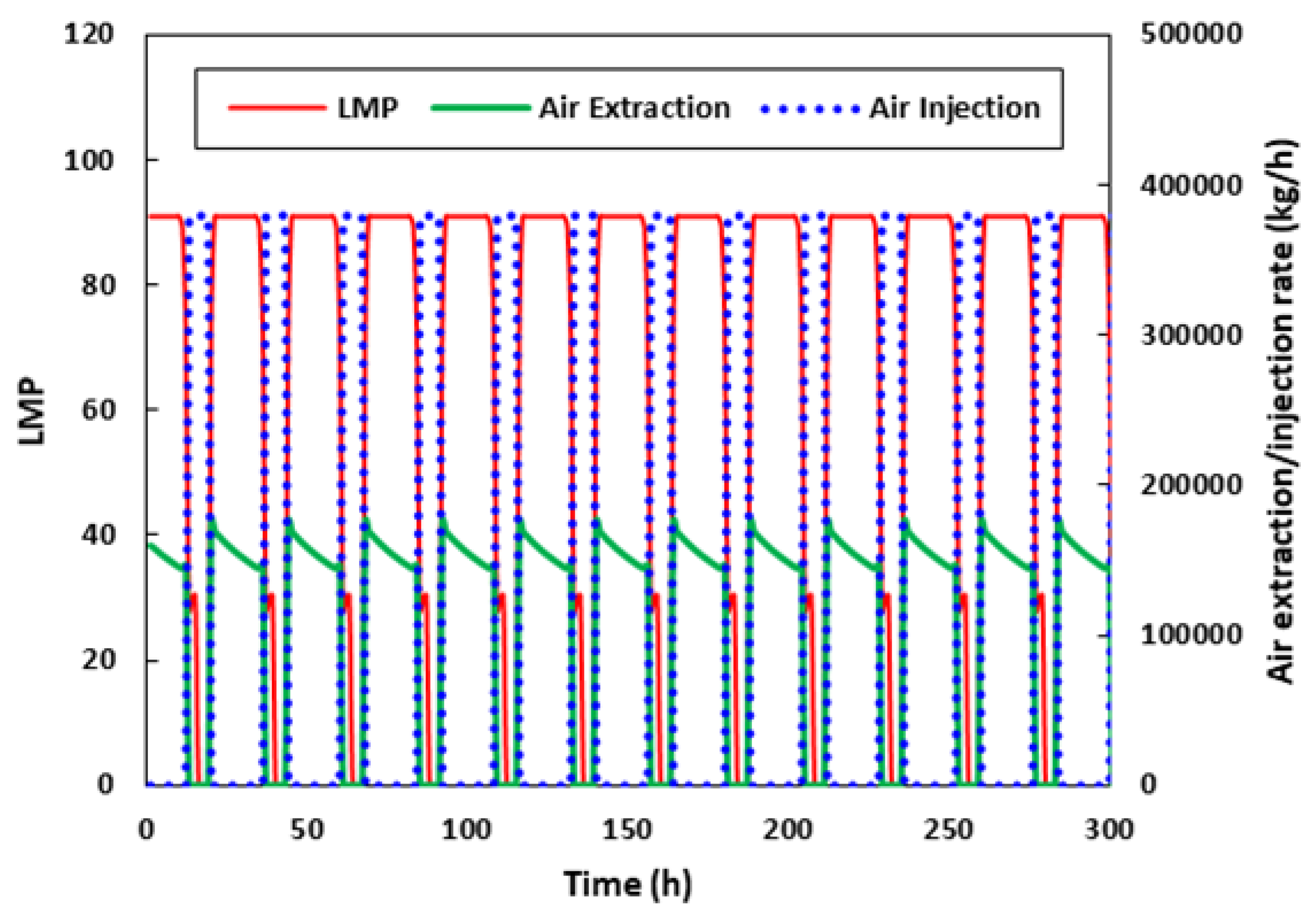
4.1. NPV Optimization

The NPV optimization is undertaken for two scenarios: NGCC only and CAES integrated with NGCC. For NGCC-only cases, the NPV optimization formulation given in Section 3.1 is modified by ignoring the constraints related to the CAES and by setting air injection and extraction flowrates to zero in the NGCC model. All cases are solved for 10 LMP data sets generated by National Renewable Energy Laboratory (NREL) and four LMP data sets from Princeton [44]. The regions in the NREL data sets are: CAISO, ERCOT, MISO, PJM, and NYISO, and for each of these regions, two tax scenarios are considered—$100/ton and $150/ton CO₂ tax. The regions in the Princeton cases are Base Case, High Solar, High Wind, and Winter NYT, where only one tax of $60/ton CO₂ is considered. These LMP data are available for 1 year with a 1 h interval and the entire LMP data set is considered for optimization.

Table 5. NPV optimization results for CAES system.

Region	Cavern Storage				LCOS-Cavern ($/MWh)
	NGCC Capacity Utilization (%)	NGCC-Only NPV ($MM)	NGCC–CAES NPV ($MM)	Cumulative Air Injection (kg)
CAISO_100	71.57	687.72	710.84	128.60 × 106	136
CAISO_150	62.87	44.23	171.33	37.64 × 106	145
ERCOT_100	60.67	−185.58	−117.08	143.77 × 106	162
ERCOT_150	68.71	−52.12	12.48	121.01 × 106	140
MISO_100	65.48	65.37	78.74	74.38 × 106	144
MISO_150	61.23	−185.58	−132.86	110.64 × 106	168
PJM_100	74.79	405.48	455.46	6.85 × 106	144
PJM_150	68.68	15.40	117.75	42.30 × 106	142
NYISO_100	59.56	335.11	345.43	57.41 × 106	144
NYISO_150	59.32	−185.58	−91.35	27.94 × 106	176
Base Case_60	88.45	322.50	376.00	142.29 × 106	142
High Solar_60	82.43	285.02	371.42	144.18 × 106	141
High Wind_60	83.09	288.17	369.21	142.62 × 106	141
Winter NYT_60	90.78	270.08	340.44	150.28 × 106	140

shows NPV optimization results for the CAES system for cavern storage where the NGCC plant capacity, NPV values for NGCC only and the integrated process (i.e., NGCC with CAES), cumulative air injection for a whole year, and LCOS are tabulated. It is observed that the optimal NGCC plant capacity utilization varies from about 59% to 91%. The maximum plant capacity utilization is obtained for the region of Princeton Winter NYT. In terms of NPV, CAISO_100, CAISO_150, MISO_100, PJM_100, PJM_150, NYISO_100, and all Princeton cases show positive NPV values for both cases. Only three regions show negative NPV for both cases, and ERCOT_150 shows negative NPV for NGCC-only cases, while the integrated process shows a positive NPV. For the integrated system, CAISO_100 yields the maximum positive NPV value of 710 $MM with the incremental NPV of 23 $MM compared to the NGCC-only case. While ERCOT_100, MISO_150, and NYISO_150 yield negative NPV for both the NGCC-only and the integrated system, the incremental NPV (i.e., NPV of the integrated process–NPV of the NGCC-only case) for the integrated process is still positive, showing that the loss was reduced by including the CAES. Figure 5 shows that the incremental NPV for all cases is positive, showing the potential of the integrated CAES system for all regions. CAISO_150 shows a maximum improvement of 127 $MM, while the second-largest improvement of 102 $MM is obtained for PJM_150. Two regions where the lowest improvements are observed are MISO_100 and NYISO_100, where the NPV improves by 13 $MM and 10 $MM, respectively.

Model profiles of two interesting cases for cavern storage, CAISO_100 and the Princeton Base Case, are briefly discussed here. Results for other regions can be found in the Appendix (Figure A1 and Figure A2). Results for the CAISO_100 region are shown in Figure 6. Figure 6a shows the variation of LMP and air injection/extraction rate versus time for thet entire year and Figure 6c shows the zoomed view of the profile for the first 300 h. The profile clearly shows that the air extraction and injection rate vary with LMP values. When the LMP price is lower, the NGCC plant operates at a part-load condition with the extent of air extraction varying depending on LMP, not only based on the instantaneous LMP but also based on the LMP of subsequent hours. Obviously, air injection will not be profitable during low-LMP-price periods, which is clearly observed from the optimal profile. During a sustained high LMP period, i.e., 80–150 $/MWh, the air injection rate reaches its maximum value of 44,662 kg/h. It is observed that, if there are low LMPs followed by a high LMP, air extraction takes place for low LMP values while injection takes place for high LMP values, as would be expected, but the flowrate for air extraction and injection at a given hour depends on the specific LMP value of that hour as well as subsequent hours. Figure 6b shows the cavern storage pressure variation. It should be noted that, even though the upper bound for the storage pressure is 72 bar, the maximum storage pressure reaches 50.7 bar for this specific case.

Results for the Princeton Base Case are shown in Figure 7. Figure 7a,c show the variation of LMP and air injection/extraction rate versus time for the entire year and zoomed view of the first 300 h, respectively, while Figure 7b shows the storage pressure variation during the entire year. The Princeton Base Case has an average (time-weighted) LMP price of 47.7 $/MWh which is lower than other regions under consideration and it also has less price variation. For both CAISO_100 and the Princeton Base Case regions, the maximum air injection rate and storage pressure are reasonably similar (about 45,000 kg/h and 50 bar). The average electricity price of the Princeton Base Case is about 10% lower than CAISO_100, but the Princeton Base Case has a 23.6% higher capacity utilization factor and 21.0% higher variable OPEX compared to CAISO_100.

In the NPV optimization formulation described in Section 3.1, roundtrip efficiency (RTE) is not explicitly taken into account as the model equations for NGCC and CAES adequately describe the system performance under design and off-design conditions. As RTE is a key performance measure of energy storage systems, it is desired to calculate RTE based on the NPV optimization results for each region. For the integrated system, RTE is calculated by using Equation (30). As the efficiency of all equipment items for the integrated NGCC–CAES system vary nonlinearly with the air extraction/injection flowrate, the yearlong profiles of these variables are used to calculate the variables in Equation (30). In Equation (30), the term $EX{P}_{CAES}$ denotes the average power production in the CAES expander per kg/s of air injected. The term ${\left(GT+ST\right)}_{NGCC}$ denotes the average power production by the GT and ST of the NGCC plant per kg/s of air injected. For calculating this term, an incremental analysis is undertaken. The power production at a given load from only NGCC without air extraction/injection is calculated. Then, the power production from the NGCC plant for a given amount of air injection flowrate is calculated. The GT compressor air flowrate is reduced by the same amount as the amount of air injected. The difference in the power production between the NGCC with and without air injection is used to calculate the power production per kg/s of air injected. The term, $HT{R}_{CAES}$, denotes the average equivalent power consumption due to the heating utility requirement per kg/s of air injected. The term $GT{C}_{NGCC}$ denotes the average power consumption in the GT compressor per kg/s of air extracted. The term ${\left(COM1+COM2\right)}_{CAES}$ denotes the average power consumption in the two-stage CAES compressor (COM1 and COM2). The term ${\left(CLR1+CLR2\right)}_{CAES}$ denotes the average equivalent power consumption in the intercoolers (CLR1 and CLR2) of the CAES system. Considering all regions, RTE is found to be 74.6–82.5%.

$${\eta }_{RTE}=\frac{Average Power Production per\frac{kg}{s}of Air Injected}{Average Power Consumption per\frac{kg}{s} of Air Extracted}=\frac{EX{P}_{CAES}+{\left(GT+ST\right)}_{NGCC}-HT{R}_{CAES}}{GT{C}_{NGCC}+{\left(COM1+COM2\right)}_{CAES}+{\left(CLR1+CLR2\right)}_{CAES}}$$

(30)

4.2. Sensitivity Analysis

Two sensitivity studies are performed to evaluate the impact of LMP and CAPEX reduction on the air extraction/injection rate and overall NPV of the CAES technology.

4.2.1. Impact of Specific LMP

The impact of the LMP is evaluated by considering an LMP profile which is intuitively ‘favorable’ for the CAES technology. For this, a specific day of CAISO_100 is selected where LMP is non-zero for most of the time and the difference of LMP in each period (24 h period) is greater than $50/MWh. Specifically, the LMP is about $30/MWh for 3 h and about $90/MWh for 15 h, and the rest are values around zero as shown in Figure 8. The entire year is assumed to have the same LMP profile. Figure 8 shows the optimal profile of air extraction/injection rate for this specific LMP. It can be seen that the maximum injection rate reaches 379,550 kg/h (as opposed to a max value of around 45,000 kg/h for CAISO_100 considering a variable LMP for all days for the entire year as presented in Section 4.1), which is about 10.5% of the total air flow (3,623,760 kg/h) into the GT compressor of the NGCC plant. The plant capacity factor improves from 72% to 81% and NPV for this case is 757 $MM, which shows a significant improvement compared to the NPV of CAISO_100 (688 $MM) presented in Section 4.1. This study suggests that the CAES technology can be an attractive investment in the region where LMP values are non-zero for most of the time, and there is a high difference between (high LMP x duration of high LMP) and (low LMP x duration of low LMP) in a period.

4.2.2. Impact of CAPEX Reduction

The impact of CAPEX reduction is analyzed by varying the CAPEX from 0 to 100%. Figure 9a,b show the effect of CAPEX reduction on the incremental cumulative air injection rate and NPV, where the incremental values are calculated by taking the differences with respect to the case without CAPEX reduction. The change in cumulative air injection and NPV is relatively flat for a CAPEX factor of 0.3 to 1.0 and, below that (0.1 to 0.3 CAPEX factor), the impact is still not substantial. Though both figures show a sharp change, the actual change is 0.04% for air injection and 0.8% for NPV and, therefore, is not substantial by considering the absolute values for cumulative air injection and NPV. This study suggests that CAPEX reduction for the case with cavern storage is likely to have a negligible impact on the economics of the CAES process.

5. Conclusions

This study sought to answer three questions listed in the ‘Introduction’ section. First, it sought to obtain the optimal design of CAES and operating conditions of the integrated system for 14 different LMP profiles by undertaking NPV optimization. The results from the optimization as well as subsequent sensitivity studies lead to the answers to the second and third questions. In response to the second question, this study finds that the NPV for the NGCC with integrated CAES is higher than the NPV for the NGCC-only cases for all regions that are studied here, thus showing that all markets have potential for the integrated CAES technology. However, the study showed that there can be considerable differences in the design and operating conditions between certain regions. For example, the cumulative air injection of CAISO_100 is about 20 times higher than PJM_100. On the other hand, the cumulative air injection for all Princeton LMP profiles and ERCOT_100 is similar. The optimal average plant capacity is found to vary from 60% to 91%, where Princeton regions consistently resulted in 88% to 91% utilization. In response to the third question, this study finds that the LMP profile has the highest impact on the economics of the integrated CAES process. A favorable LMP profile is observed when LMP values are non-zero for most of the time, and there is a high difference between (high LMP x duration of high LMP) and (low LMP x duration of low LMP). CAPEX reduction is observed to have a negligible effect on the air injection/extraction rates and overall plant economics. LCOS is another indicator for a feasible market. Here, LCOS for the cavern storage is mostly in the range of 136–145 $/MWh except ERCOT_100, MISO_150, and NYISO_150, where the LCOS is in the range of 162–176 $/MWh. Another key performance measure of an energy storage system is RTE, which is found to vary between 74.6–82.5%. Overall, the study shows that the integration of CAES into the NGCC plant can be an economically viable option for energy storage for many regions given the appropriate LMP profile.

References

1. WEC. World Energy Focus 2014, World Energy Leaders’ Summit and Executive Assembly of the World Energy Council, October 2104, Cartagena, Colombia. Available online: https://www.worldenergy.org/assets/downloads/WEC-Annual-2014-Web-01.pdf (accessed on 25 February 2023).
2. Berrill, P. Life Cycle Assessment of Power Systems with Large Shares of Variable Renewable Energy. Master’s Thesis, University of Graz, Graz, Austria, 2015. [Google Scholar]
3. Heidari, M.; Parra, D.; Patel, M.K. Physical design, techno-economic analysis and optimization of distributed compressed air energy storage for renewable energy integration. J. Energy Storage 2021, 35, 102268. [Google Scholar] [CrossRef]
4. Ibrahim, H.; Ilinca, A. Techno-Economic Analysis of Different Energy Storage Technologies. In Energy Storage—Technologies and Applications; Zobaa, A.F., Ed.; IntechOpen: London, UK, 2013; pp. 1–40. [Google Scholar] [CrossRef] [Green Version]
5. Zhou, Q.; Du, D.; Lu, C.; He, Q.; Liu, W. A review of thermal energy storage in compressed air energy storage system. Energy 2019, 188, 115993. [Google Scholar] [CrossRef]
6. Celsius. Thermal Energy Storage—Overview and Basic Principles. Available online: https://celsiuscity.eu/thermal-energy-storage/ (accessed on 25 February 2023).
7. Raju, M.; Khaitan, S.K. Modeling and simulation of compressed air storage in caverns: A case study of the Huntorf plant. Applied Energy 2012, 89, 474–481. [Google Scholar] [CrossRef]
8. King, M.; Jain, A.; Bhakar, R.; Mathur, J.; Wang, J. Overview of current compressed air energy storage projects and analysis of the potential underground storage capacity in India and the UK. Ren. Sust. Energy Rev. 2021, 139, 110705. [Google Scholar] [CrossRef]
9. Staubly, R.K.; Pedrick, G.A.; Seneca Compressed Air Energy Storage (CAES) Project. Final Phase 1 Technical Report for National Energy Technology Laboratory (NETL). September 2012. Available online: https://www.energy.gov/sites/prod/files/2016/12/f34/NETL-Final-Report-9-6-12.pdf (accessed on 12 April 2023).
10. Wang, Y.; Bhattacharyya, D.; Turton, R. Evaluation of Novel Configurations of Natural Gas Combined Cycle (NGCC) Power Plants for Load-Following Operation using Dynamic Modeling and Optimization. Energy Fuels 2020, 34, 1053–1070. [Google Scholar] [CrossRef]
11. Wang, Y. Quantifying the Impact of Load-Following on Gas-fired Power Plants Quantifying the Impact of Load-Following on Gas-Fired Power Plants Department of Chemical and Biomedical Engineering. Ph.D. Thesis, West Virginia University, Morgantown, WV, USA, 2021. [Google Scholar]
12. Budt, M.; Wolf, D.; Span, R.; Yan, J. A review on compressed air energy storage: Basic principles, past milestones and recent developments. Appl. Energy 2016, 170, 250–268. [Google Scholar] [CrossRef]
13. Peng, H.; Yang, Y.; Li, R.; Ling, X. Thermodynamic analysis of an improved adiabatic compressed air energy storage system. Appl. Energy 2016, 183, 1361–1373. [Google Scholar] [CrossRef]
14. Kéré, A.; Goetz, V.; Py, X.; Olives, R.; Sadiki, N. Modeling and integration of a heat storage tank in a compressed air electricity storage process. Energy Conv. Manag. 2015, 103, 499–510. [Google Scholar] [CrossRef]
15. Guo, C.; Xu, Y.; Zhang, X.; Guo, H.; Zhou, X.; Liu, C.; Qin, W.; Li, W.; Dou, B.; Chen, H. Performance analysis of compressed air energy storage systems considering dynamic characteristics of compressed air storage. Energy 2017, 135, 876–888. [Google Scholar] [CrossRef]
16. Wolf, D.; Budt, M. LTA-CAES—A low-temperature approach to adiabatic compressed air energy storage. Appl. Energy 2014, 125, 158–164. [Google Scholar] [CrossRef]
17. Guo, Z.; Deng, G.; Fan, Y.; Chen, G. Performance optimization of adiabatic compressed air energy storage with ejector technology. Appl. Therm. Eng. 2016, 94, 193–197. [Google Scholar] [CrossRef]
18. Jeong, J.H.; Yi, J.H.; Kim, T.S. Analysis of options in combining compressed air energy storage with a natural gas combined cycle. J. Mech. Sci. Technol. 2018, 32, 3453–3464. [Google Scholar] [CrossRef]
19. Brooks, F.J. GE Gas Turbine Performance Characteristics. Available online: https://www.ge.com/content/dam/gepower-new/global/en_US/downloads/gas-new-site/resources/reference/ger-3567h-ge-gas-turbine-performance-characteristics.pdf (accessed on 10 April 2023).
20. Igie, U.; Abbondanza, M.; Szymanski, A.; Nikolaidis, T. Impact of compressed air energy storage demands on gas turbine performance. Proc. IMechE Part A J. Power Energy 2021, 235, 850–865. [Google Scholar] [CrossRef] [Green Version]
21. Wojcik, J.D.; Wang, J. Feasibility study of combined cycle gas turbine (CCGT) power plant integration with adiabatic compressed air energy storage (ACAES). Appl. Energy 2018, 221, 477–489. [Google Scholar] [CrossRef]
22. Kruk-Gotzman, S.; Ziolkowski, P.; Iliev, I.; Negreanu, G.-P.; Badur, J. Techno-economic evaluation of combined cycle gas turbine and a diabatic compressed air energy storage integration concept. Energy 2023, 266, 126345. [Google Scholar] [CrossRef]
23. Salvini, C. Techno-Economic Analysis of CAES systems Integrated into Gas-Steam Combined Plants. Energy Procedia 2016, 101, 870–877. [Google Scholar] [CrossRef]
24. He, X.; Li, C.C.; Wang, H. Thermodynamics analysis of a combined cooling, heating and power system integrating compressed air energy storage and gas-steam combined cycle. Energy 2022, 260, 125105. [Google Scholar] [CrossRef]
25. Sokhanvar, K.; Karimpour, A.; Pariz, N. Electricity price forecasting using a clustering approach. In Proceedings of the 2nd IEEE International Conference on Power and Energy, Johor Bahru, Malaysia, 1–3 December 2008. [Google Scholar] [CrossRef]
26. Mosher, T. Economic Valuation of Energy Storage Coupled with Photovoltaics: Current Technologies and Future Projections. Master’s Thesis, Massachusetts Institute of Technology, Cambridge, MA, USA, 2010. [Google Scholar]
27. Simpore, S.; Garde, F.; David, M.; Marc, O.; Castaing-Lasvignottes, J. Design and Dynamic Simulation of a Compressed Air Energy Storage System (CAES) Coupled with a Building, an Electric Grid and a Photovoltaic Power Plant. In Proceedings of the CLIMA 2016—proceedings of the 12th REHVA World Congress, Aalborg, Denmark, 22–25 May 2016; Available online: https://vbn.aau.dk/files/233718244/paper_651.pdf (accessed on 25 February 2023).
28. Saada, M.; Shiraz, F.A.; Li, P.Y. Revenue Maximization of Electricity Generation for a Wind Turbine Integrated with a Compressed Air Energy Storage System. In Proceedings of the 2014 American Control Conference (ACC), Portland, Oregon, 4–6 June 2014; Available online: https://ieeexplore.ieee.org/stamp/stamp.jsp?tp=&arnumber=6859445&tag=1 (accessed on 25 February 2023).
29. Desai, N. The Economic Impact of CAES on Wind in TX, OK, and NM. 2005. Available online: https://www.sandia.gov/files/ess/EESAT/2005_papers/Jewitt-Desai_CAES.pdf (accessed on 25 February 2023).
30. Cleary, B. A Techno-Economic Analysis of Wind Generation in Conjunction with Compressed Air Energy Storage in the Integrated Single Electricity Market. Ph.D. Thesis, Technological University Dublin, Dublin, Ireland, 2016. [Google Scholar] [CrossRef]
31. Cheng, J. Configuration and Optimization of a Novel Compressed-Air-Assisted Wind Energy Conversion System. Ph.D. Thesis, University of Nebraska, Lincoln, NE, USA, 2016. [Google Scholar]
32. Luo, X.; Wang, J.; Krupke, C.; Wang, Y.; Sheng, Y.; Li, J.; Xu, Y.; Wang, D.; Miao, S.; Chen, H. Modelling study, efficiency analysis and optimisation of large-scale Adiabatic Compressed Air Energy Storage systems with low-temperature thermal storage. Appl. Energy 2016, 162, 589–600. [Google Scholar] [CrossRef]
33. Fu, Z.; Lu, K.; Zhu, Y. Thermal system analysis and optimization of large-scale compressed air energy storage (CAES). Energies 2015, 8, 8873–8886. [Google Scholar] [CrossRef] [Green Version]
34. Gu, Y.; McCalley, J.; Ni, M.; Bo, R. Economic modeling of compressed air energy storage. Energies 2013, 6, 2221–2241. [Google Scholar] [CrossRef]
35. Shamshirgaran, S.R.; Ameri, M.; Khalaji, M.; Ahmadi, M.H. Design and optimization of a compressed air energy storage (CAES) power plant by implementing genetic algorithm. Mech. Ind. 2016, 17, 109. [Google Scholar] [CrossRef]
36. Zoelle, A.; Keairns, D.; Pinkertin, L.L.; Turner, M.J.; Woods, M.; Kuehn, N.; Shah, V.; Chou, V. Cost and Performance Baseline for Fossil Energy Plants Vol. 1a: Bituminous Coal (PC) and Natural Gas to Electricity Revision 3; DOE/NETL-2015/1723; National Energy Technology Laboratory: Pittsburgh, PA, USA; Morgantown, WV, USA, 2015; pp. 1–240. Available online: https://www.osti.gov/biblio/1480987 (accessed on 10 April 2023).
37. Chen, L.; Zheng, T.; Mei, S.; Xue, X.; Liu, B.; Lu, Q. Review and prospect of compressed air energy storage system. J. Mod. Power Syst. Clean Energy 2016, 4, 529–541. [Google Scholar] [CrossRef] [Green Version]
38. Crotogino, F.; Mohmeyer, K.U.; Scharf, R. Huntorf CAES: More than 20 Years of Successful Operation. In Proceedings of the Solution Mining Research Institute Spring Meeting, Orlando, FL, USA, 23–25 April 2001. [Google Scholar]
39. Paul, P.; Bhattacharyya, D.; Turton, R.; Zitney, S.E. Nonlinear Dynamic Model-Based Multiobjective Sensor Network Design Algorithm for a Plant with an Estimator-Based Control System. Ind. Eng. Chem. Res. 2017, 56, 7478–7490. [Google Scholar] [CrossRef]
40. Turton, R.; Shaeiwitz, J.A.; Bhattacharyya, D.; Whiting, W.B. Analysis, Synthesis, and Design of Chemical Processes, 5th ed.; Prentice Hall: Hoboken, NJ, USA, 2018. [Google Scholar]
41. Mongird, K.; Viswanathan, V.; Alam, J.; Vartanian, C.; Sprenkle, V.; Northwest, P. 2020 Grid Energy Storage Technology Cost and Performance Assessment. NETL. December 2020. Available online: https://www.pnnl.gov/sites/default/files/media/file/Final%20-%20ESGC%20Cost%20Performance%20Report%2012-11-2020.pdf (accessed on 25 February 2023).
42. Bynum, M.L.; Hackebeil, G.A.; Hart, W.E.; Laird, C.D.; Nicholson, B.L.; Siirola, J.D.; Watson, J.P.; Woodruff, D.L. Pyomo—Optimization Modeling in Python, 3rd ed.; Springer: Berlin/Heidelberg, Germany, 2021. [Google Scholar]
43. Sadhukhan, J.; Sen, S.; Randriamahefasoa, T.M.S.; Gadkari, S. Energy System Optimization for Net-Zero Electricity. Dig. Chem. Eng. 2022, 3, 100026. [Google Scholar] [CrossRef]
44. Sun, Y.; Wachche, S.; Mills, A.; Ma, O.; Meshek, M.; Buchanan, S.; Hicks, A.; Roberts, B. 2018 Renewable Energy Grid Integration Data Book; National Renewable Energy Laboratory: Golden, CO, USA, 2020. [Google Scholar]
Figure 1. Schematic representation of CAES system integrated with NGCC plant.
Energies 16 04867 g001
Figure 2. Model validation results: (a) dynamics of mass flowrate; (b) pressure change in the cavern; and (c) temperature change in the cavern.
Energies 16 04867 g002
Figure 3. Simulated inputs for testing the ROM performance: (a) natural gas flowrate, (b) air extraction flowrate, (c) air injection flowrate, and (d) air injection temperature.
Energies 16 04867 g003
Figure 4. Comparison between APD/FOM/ROM: (a) net power output; (b) LP steam extraction temperature; (c) steam turbine output; and (d) CO2 mass flowrate in flue gas.
Energies 16 04867 g004
Figure 5. Incremental NPV for the CAES system for cavern storage.
Energies 16 04867 g005
Figure 6. Optimization results for CAISO_100 region: (a) air extraction and injection profile, (b) cavern storage pressure profile, and (c) zoomed view of air extraction and injection profile.
Energies 16 04867 g006
Figure 7. Optimization results for Princeton Base Case_60 region: (a) air extraction and injection profile, (b) cavern storage pressure profile, and (c) zoomed view of air extraction and injection profile.
Energies 16 04867 g007
Figure 8. Air extraction and injection profile for a specific LMP.
Energies 16 04867 g008
Figure 9. Effect of CAPEX reduction on the (a) incremental cumulative air injection, and (b) incremental NPV.
Energies 16 04867 g009