The Dynamics of US Gasoline Demand and Its Prediction: An Extended Dynamic Model Averaging Approach

Abstract

This study contributes to the body of literature on modeling and predicting gasoline demand by using nonlinear econometric techniques. For this purpose, dynamic model averaging (DMA) and Bayesian model averaging (BMA) combined with Artificial Bee Colony (ABC) are used to forecast gasoline consumption in the United States. The article’s independent variables include demographic characteristics, economic activity, income, driving expenditures, automobile price, and road availability for annual data from 1960 to 2020. In the proposed model, not only may the coefficients and elasticity of a predictor of gasoline demand change over time, but other sets of predictors can also emerge at different periods. Moreover, this study aims to automate the process of picking two forgotten variables of the DMA model using the ABC model. Our findings indicate that dynamic model averaging significantly improves forecasting performance when compared to basic benchmark techniques and advanced approaches. Additionally, integrating it with an Artificial Bee Colony (ABC) may result in improved outcomes when time-varying forgetting variables are present. The findings of this research provide policymakers in the fields of energy economics and the environment with helpful tools and information.

1. Introduction

Gasoline demand in the United States has been steadily increasing since the 1990s. In 2019, Approximately 143 billion gallons of gasoline was used in the United States, with the transportation sector accounting for over 70% of the total consumption [1]. The demand increase can be attributed to factors, such as population growth, urbanization, and increased consumer spending on vehicles. Furthermore, the EIA [1] reported that gasoline demand is highly sensitive to changes in economic activity, fuel prices, and weather patterns. For example, during the COVID-19 pandemic in 2020, gasoline demand in the US fell significantly due to reduced economic activity and stay-at-home orders. However, as the economy recovers and restrictions are lifted, demand is expected to increase once again. In addition, the EIA [1] predicts that gasoline demand will continue to rise in the coming years, reaching approximately 151 billion gallons by 2050.

Numerous research has been conducted on the effectiveness of gasoline demand factors and their capacity to forecast. In this context, some previous studies have adopted a direct approach to estimation by examining the demand for car sales [2,3,4,5]. Apart from forecasting vehicle sales, research in the area of travel demand has also looked at gasoline use as a response variable when evaluating fuel price elasticities [6,7,8,9]. Huo and Wang [5] discovered that pricing and income elasticities in China are based on consumer vehicle stock and projected vehicle sales in China up to 2050 using the FEEI model. Bento et al. [10] conducted similar research for the United States, using a simultaneous equations model for US households and taking into account the new discarded vehicle markets, among other factors. Graham and Glaister [9] conducted a thorough literature review of 113 studies conducted in the United Kingdom. Goetzke and Vance [11] and Bento et al. [10] found comparable results in terms of fuel consumption’s reactivity to fuel prices and in contrast to vehicle mile travel’s response to fuel prices. Meanwhile, Oladosu [6] described individual family fuel consumption choices using a vehicle–fuel expenditure allocation model (or AIDS model) for multi-vehicle families in the United States.

In addition, there is a lack of consensus on the estimated coefficients in the studies that have been carried out in the process of modeling and predicting gasoline demand. According to Goetzke and Vance’s [11] review of the literature, the average gasoline price elasticity is roughly −0.18, with estimates ranging from −1.01 to 0.01. Thus, the majority of studies interpret these fuel price elasticities as evidence for the existence of a rebound effect, in which the cost savings associated with a reduction in the cost of driving or a gain in fuel efficiency eventually result in an unforeseen rise in fuel consumption. The rebound effect describes a situation in which drivers are presented with lower travel costs (such as falling gas prices) and/or increased fuel efficiency, which unintentionally results in increased fuel consumption and/or vehicle travel. Consequently, in terms of policy, such a phenomenon might result in erroneous calculations and, thus, incorrect interpretations for decision makers. Dimitropoulos et al. [12] conducted a meta-analysis of 74 studies that included 1120 estimates of reported rebound effects and discovered an average rebound effect of 10% to 12%. This unintended impact on driving and fuel consumption habits has significant consequences for the efficacy of policy planning and interventions aimed at reducing emissions and fuel consumption. Overall, studies in the transportation literature employ a variety of methods in terms of model selection, with the majority of scholars being aware of obvious causes for observed discrepancies in the findings. As a result, the effective modeling and forecasting of gasoline demand may offer a critical foundation for policymakers to consider the policy implications of their energy market activities, which is the goal of this paper.

At a minimum, typical forecasting models have two shortcomings: first, numerous studies have shown that predictors change over time, and factors, such as market cycles and macroeconomic policy changes, may result in structural breakdowns in the relationship between fundamental principles and dynamics. Additionally, the effect of each input on the dependent variable changes according to the period and market conditions [13,14]. A model with a static list of predictors may also lose accuracy and consistency over time. Extensive and precise analysis may be performed at any time to pick a model. In other words, if we have $N$ predictors, we must evaluate and compare, $2^N$ models at each time point (the number of subsets of $N$ variables that accurately represent all possible combinations and inclusions of $N$ variables in the model) with $T\times 2^N$ as the total number of models should be tested throughout T. Therefore, while N and T are large, their analysis is impossible or, at least, difficult.

The accuracy of forecasts has been improved by using model averaging approaches, such as “forecasting combination”, in recent research. Both “Bayesian Model Averaging” (BMA) and “ forecasting combination” models are characterized by fixed weight values given to models throughout time; however, they do not offer sufficient flexibility to manage the time gap between the contributions of the modeling [15,16]. Therefore, dynamic model selection (DMS) and dynamic model averaging (DMA) were suggested by Raftery et al. [17] to overcome the limitations of the other models. Findings show that macroeconomic forecasting may benefit from this method [18,19]. The appropriateness of each model throughout time is shown in several studies on this subject. The time-varying parameter (TVP) model may employ DMA to compute the average likelihood of each variable being present in the best prediction model. As a more exact definition, one may argue that the average forecast across models is based on an average likelihood of the existence of a variable at time t based on prior knowledge [19,20,21]. Selecting the optimal prediction model is based on determining which variables have the greatest likelihood of being present in this model, and the model’s prediction will be based on this calculation [19]. Although DMS picks a model that comprises variables most likely to be included in forecast models among those estimated in each period, it does so in a more efficient manner. Inspired by the works of Koop and Korobilis [18] and Bork and Mller [22], Raftery et al. [17] found that the DMA model’s forecasting accuracy was 30 percent higher than that of other time-series approaches, such as AR and OLS regression. A DMA technique is presented by Wei and Cao [23] to predict a housing price increase in Chinese cities. Research shows that DMA is a better forecasting model than BMA, equal-weighted averaging (EW), and information-theoretic modeling. Dong and Yoon [24] employed a DMA approach to explore the global economic drivers that have a large impact on developing Asian stock market returns, notably during the financial crisis. Moreover, other applications for predicting are noteworthy: aggregate equity returns [25], commodity prices [26,27], exchange rates [28,29], Government bond yields’ term structure [27], and commodity price volatility and equity return [30].

Therefore, the following is the study’s primary contributions: (1) This study aims to estimate and forecast the gasoline demand in the USA using TVP techniques, particularly the DMA approach, which is much more accurate than prior methods. (2) In most investigations, Bayesian TVP is used to estimate the model’s parameters [31,32]. Although this approach approximates the generation of model parameters and switching probabilities using two forgetting elements, the inclusion of forgotten factors might be helpful since full Bayesian models may be quite large and time consuming in terms of computational volume. It also assumes that the two factors are constant over time, which is not the case for the single mechanism addressed in the study by Koop and Korobilis [18]. In addition, removing this constraint to reduce the computing cost of the model may lead to an improvement in model prediction accuracy. In this study, we attempt to execute a random process of forgetting factor selection using an algorithm called the ABC. Therefore, another key contribution in this work is to integrate ABC with DMA to improve the forecast accuracy.

The remaining parts of the article are organized as described below. In the second section, a research approach is presented. In Section 3, we provide a summary of both our data and the empirical findings of the forecasting. The conclusion is presented in Section 5.

2. Research Methodology

The DMA technique employed in the study at hand was introduced by Raftery et al. [17]. The following is the standard models for State-Space approaches, namely the Kalman filter:

$${\mathrm{y}}_{\mathrm{t}}={\mathrm{z}}_{\mathrm{t}}{\mathsf{\theta }}_{\mathrm{t}}+{\mathsf{\epsilon }}_{\mathrm{t}}$$

(1)

$${\mathsf{\theta }}_{\mathrm{t}}={\mathsf{\theta }}_{\mathrm{t}-1}+{\mathsf{\mu }}_{\mathrm{t}}$$

(2)

where ${\mathsf{\theta }}_{\mathrm{t}}=\left[{\mathsf{\phi }}_{\mathrm{t}-1},{\mathsf{\beta }}_{\mathrm{t}-1},{\mathsf{\gamma }}_{\mathrm{t}-1},\cdots ,{\mathsf{\gamma }}_{\mathrm{t}-\mathrm{p}}\right]$ denotes a vector of $\mathrm{m}\times 1$ coefficients, and ${\mathsf{\mu }}_{\mathrm{t}}~\mathrm{N}(0,{\mathrm{Q}}_{\mathrm{t}})$ and ${\mathsf{\epsilon }}_{\mathrm{t}}~\mathrm{N}(0,{\mathrm{H}}_{\mathrm{t}})$ with a mean of zero and variances of ${\mathrm{Q}}_{\mathrm{t}}$ and ${\mathrm{H}}_{\mathrm{t}}$ are normally distributed. ${\mathrm{y}}_{\mathrm{t}}$ denotes a dependent variable, and ${\mathrm{z}}_{\mathrm{t}}=\left[1,{\mathrm{x}}_{\mathrm{t}-1},{\mathrm{y}}_{\mathrm{t}-1},\cdots ,{\mathrm{y}}_{\mathrm{t}-\mathrm{p}}\right]$ denotes a $1\times \mathrm{m}$ vector of variable interruption and intercept estimators depending on the model. As a consequence, the State-Space method is defined as follows, given a subset of K models at a given time:

$${\mathrm{y}}_{\mathrm{t}}={\mathrm{z}}_{\mathrm{t}}^{\left(\mathrm{k}\right)}{\mathsf{\theta }}_{\mathrm{t}}^{\left(\mathrm{k}\right)}+{\mathsf{\epsilon }}_{\mathrm{t}}^{\left(\mathrm{k}\right)}$$

(3)

$${\mathsf{\theta }}_{\mathrm{t}+1}^{\left(\mathrm{k}\right)}={\mathsf{\theta }}_{\mathrm{t}}^{\left(\mathrm{k}\right)}+{\mathsf{\mu }}_{\mathrm{t}}^{\left(\mathrm{k}\right)}$$

(4)

In this equation, ${\mathsf{\epsilon }}_{\mathrm{t}}^{\left(\mathrm{k}\right)}~\mathrm{N}(0,{\mathrm{H}}_{\mathrm{t}}^{\left(\mathrm{k}\right)})$ and ${\mathsf{\mu }}_{\mathrm{t}}^{\left(\mathrm{k}\right)}~\mathrm{N}(0,{\mathrm{Q}}_{\mathrm{t}}^{\left(\mathrm{k}\right)})$ with ${\mathsf{\vartheta }}_{\mathrm{t}}=({\mathsf{\theta }}_{\mathrm{t}}^{\left(1\right)},\cdots ,{\mathsf{\theta }}_{\mathrm{t}}^{\left(\mathrm{k}\right)})$ reveal which model of K subsets performs best during whatever period. Dynamic model averaging is a technique that permits a distinct model to be estimated at every given moment [19]. Raftery et al. [17] proposed a DMA approach that involves two parameters of $\mathsf{\alpha }$ and $\mathsf{\lambda }$, dubbed the forgetting factors. A recurrence estimate or forecast is feasible based on the information of conventional filtering when the constants ${\mathrm{H}}_{\mathrm{t}}$ and ${\mathrm{Q}}_{\mathrm{t}}$ are being considered. The following formula serves as the foundation for the Kalman filtering (KF) process:

$${\mathsf{\theta }}_{\mathrm{t}-1}\left|{\mathrm{y}}^{\mathrm{t}-1}\right.~\mathrm{N}({\widehat{\mathsf{\theta }}}_{\mathrm{t}-1},{\sum }_{\mathrm{t}-1\left|\mathrm{t}-1\right.})$$

(5)

In Equation (5), the calculation of ${\sum }_{\mathrm{t}-1\left|\mathrm{t}-1\right.}$ and ${\widehat{\mathsf{\theta }}}_{\mathrm{t}-1}$ is performed using a conventional approach that is a function of ${\mathrm{H}}_{\mathrm{t}}$ and ${\mathrm{Q}}_{\mathrm{t}}$, and then the KF process is performed using the following equation:

$${\mathsf{\theta }}_{\mathrm{t}}\left|{\mathrm{y}}^{\mathrm{t}-1}\right.~\mathrm{N}({\widehat{\mathsf{\theta }}}_{\mathrm{t}-1},{\sum }_{\mathrm{t}\left|\mathrm{t}-1\right.})$$

(6)

Since ${\sum }_{\mathrm{t}\left|\mathrm{t}-1\right.}={\sum }_{\mathrm{t}-1\left|\mathrm{t}-1\right.}+{\mathrm{Q}}_{\mathrm{t}}$, to simplify, Raftery et al. [17] substituted ${\sum }_{\mathrm{t}\left|\mathrm{t}-1\right.}=\frac{1}{{\mathsf{\lambda }}_{\mathrm{t}\left|\mathrm{t}-1\right.}}{\sum }_{\mathrm{t}-1\left|\mathrm{t}-1\right.}$ with ${\sum }_{\mathrm{t}\left|\mathrm{t}-1\right.}={\sum }_{\mathrm{t}-1\left|\mathrm{t}-1\right.}+{\mathrm{Q}}_{\mathrm{t}}$, accordingly with $0<\mathsf{\lambda }\le 1$, ${\mathrm{Q}}_{\mathrm{t}}=(1-{{\mathsf{\lambda }}_{\mathrm{t}\left|\mathrm{t}-1\right.}}^{-1}){\sum }_{\mathrm{t}-1\left|\mathrm{t}-1\right.}$. The value of ${\mathsf{\lambda }}_{\mathrm{t}}$ that is near to one suggests that the coefficients change more gradually. Raftery et al. [17] awarded it a value of 0.99 for the last five years’ quarterly statistical data; the preceding figure shows that the observations from the previous five years account for 80 percent of the most current observation. If it is 95%, it indicates that the most recent five years of data accounted for 35% of the weight of the earlier observation. As a result, it is critical to choose the forgetting factors, which are often believed to be between 95 and 99 percent. The estimate in the model will be completed by using updated estimators using the following functions:

$${\mathsf{\lambda }}_{\mathrm{t}\left|\mathrm{t}\right.}={\mathsf{\lambda }}_{\mathrm{t}-1\left|\mathrm{t}-1\right.}$$

$${\mathsf{\theta }}_{\mathrm{t}}\left|{\mathrm{y}}^{\mathrm{t}}\right.~\mathrm{N}({\widehat{\mathsf{\theta }}}_{\mathrm{t}},{\sum }_{\mathrm{t}\left|\mathrm{t}\right.})$$

(7)

In which

$${\widehat{\mathsf{\theta }}}_{\mathrm{t}}={\widehat{\mathsf{\theta }}}_{\mathrm{t}-1}+{\sum }_{\mathrm{t}\left|\mathrm{t}-1\right.}{\mathrm{z}}_{\mathrm{t}}{\left({\mathrm{H}}_{\mathrm{t}}+{\mathrm{z}}_{\mathrm{t}}{\sum }_{\mathrm{t}\left|\mathrm{t}-1\right.}{\mathrm{z}}_{\mathrm{t}}^{\prime }\right)}^{-1}({\mathrm{y}}_{\mathrm{t}}-{\mathrm{z}}_{\mathrm{t}}{\widehat{\mathsf{\theta }}}_{\mathrm{t}-1})$$

(8)

$${\sum }_{\mathrm{t}\left|\mathrm{t}\right.}={{\sum }_{\mathrm{t}\left|\mathrm{t}-1\right.}-{\sum }_{\mathrm{t}\left|\mathrm{t}-1\right.}{\mathrm{z}}_{\mathrm{t}}{\left({\mathrm{H}}_{\mathrm{t}}+{\mathrm{z}}_{\mathrm{t}}{\sum }_{\mathrm{t}\left|\mathrm{t}-1\right.}{\mathrm{z}}_{\mathrm{t}}^{\prime }\right)}^{-1}{\mathrm{z}}_{\mathrm{t}}{\sum }_{\mathrm{t}\left|\mathrm{t}-1\right.}}_{}$$

(9)

Recursive prediction operates based on the predictive distribution in the following manner:

$$\left.{\mathrm{y}}_{\mathrm{t}}\right|{\mathrm{y}}^{\mathrm{t}-1}~\mathrm{N}\left({\mathrm{z}}_{\mathrm{t}}{\widehat{\mathsf{\theta }}}_{\mathrm{t}-1}{,\mathrm{H}}_{\mathrm{t}}+{\mathrm{z}}_{\mathrm{t}}{\sum }_{\mathrm{t}\left|\mathrm{t}-1\right.}{\mathrm{z}}_{\mathrm{t}}^{\mathrm{’}}\right)$$

(10)

Depending on the model, the above-mentioned functions for k may be expressed as follows, whereas the KF in the fixed estimators’ model can be represented as (5)–(7), using ${\mathsf{\vartheta }}_{\mathrm{t}}$ as a vector of all parameters (3) and (4).

$${\mathsf{\vartheta }}_{\mathrm{t}-1}\left|{\mathrm{L}}_{\mathrm{t}-1}=\mathrm{k},{\mathrm{y}}^{\mathrm{t}-1}~\mathrm{N}({\widehat{\mathsf{\theta }}}_{\mathrm{t}-1}^{\left(\mathrm{k}\right)},{\sum }_{\mathrm{t}-1\left|\mathrm{t}-1\right.}^{\left(\mathrm{k}\right)})\right.$$

(11)

$${\mathsf{\vartheta }}_{\mathrm{t}}\left|{\mathrm{L}}_{\mathrm{t}}=\mathrm{k},{\mathrm{y}}^{\mathrm{t}-1}~\mathrm{N}({\widehat{\mathsf{\theta }}}_{\mathrm{t}-1}^{\left(\mathrm{k}\right)},{\sum }_{\mathrm{t}\left|\mathrm{t}-1\right.}^{\left(\mathrm{k}\right)})\right.$$

(12)

$${\mathsf{\vartheta }}_{\mathrm{t}}\left|{\mathrm{L}}_{\mathrm{t}}=\mathrm{k},{\mathrm{y}}^{\mathrm{t}}~\mathrm{N}({\widehat{\mathsf{\theta }}}_{\mathrm{t}}^{\left(\mathrm{k}\right)},{\sum }_{\mathrm{t}\left|\mathrm{t}\right.}^{\left(\mathrm{k}\right)})\right.$$

(13)

The value of ${\widehat{\mathsf{\theta }}}_{\mathrm{t}}^{\left(\mathrm{k}\right)}$ and $({\sum }_{\mathrm{t}\left|\mathrm{t}\right.}^{\left(\mathrm{k}\right)})$ and $({\sum }_{\mathrm{t}\left|\mathrm{t}-1\right.}^{\left(\mathrm{k}\right)})$ was acquired with the use of KF and Equations (8) and (9) and ${\sum }_{\mathrm{t}\left|\mathrm{t}-1\right.}=\frac{1}{{\mathsf{\lambda }}_{\mathrm{t}\left|\mathrm{t}-1\right.}}{\sum }_{\mathrm{t}-1\left|\mathrm{t}-1\right.}$. We employed the Raftery et al. [17] technique, which incorporates a forgetting factor termed $\mathsf{\alpha }$ for state equations in various estimating models, and so the aforementioned components are analogous to the forgetting factor. Equation (4) is the starting point for the Kalman filter’s application. When DMA is utilized, similar effects are obtained:

$${\mathrm{P}(\mathsf{\vartheta }}_{\mathrm{t}-1}\left|{\mathrm{y}}^{\mathrm{t}-1}\right.)={\sum }_{\mathrm{k}=1}^{\mathrm{K}}\mathrm{p}({\mathsf{\theta }}_{\mathrm{t}-1}^{\left(\mathrm{k}\right)}\left|{\mathrm{L}}_{\mathrm{t}-1}=\mathrm{k},{\mathrm{y}}^{\mathrm{t}-1})\mathrm{Pr}\left({\mathrm{L}}_{\mathrm{t}-1}=\mathrm{k}\left|{\mathrm{y}}^{\mathrm{t}-1}\right.\right)\right.$$

(14)

The model’s prediction function was replaced by the following equation introduced by Raftery et al. [17].

$${\mathsf{\pi }}_{\mathrm{t}⌊\mathrm{t}-1,\mathrm{k}}=\frac{{\mathsf{\pi }}_{\mathrm{t}-1\left|\mathrm{t}-1,\mathrm{k}\right.}^{{\mathsf{\alpha }}_{\mathrm{t}\left|\mathrm{t}-1\right.}}}{\sum _{\mathrm{l}=1}^{\mathrm{K}}{\mathsf{\pi }}_{\mathrm{t}-1\left|\mathrm{t}-1,\mathrm{l}\right.}^{{\mathsf{\alpha }}_{\mathrm{t}\left|\mathrm{t}-1\right.}}}$$

(15)

If $0\le \mathsf{\alpha }<1$, the interpretation will be identical to that of $\mathsf{\lambda },$ resulting in the following updated function:

$${\mathsf{\pi }}_{\mathrm{t}⌊\mathrm{t},\mathrm{k}}=\frac{{\mathsf{\pi }}_{\mathrm{t}⌊\mathrm{t}-1,\mathrm{k}}^{{\mathsf{\alpha }}_{\mathrm{t}\left|\mathrm{t}-1\right.}}{\mathrm{p}}_{\mathrm{k}}({\mathrm{y}}_{\mathrm{t}}\left|{\mathrm{y}}^{\mathrm{t}-1})\right.}{\sum _{\mathrm{l}=1}^{\mathrm{K}}{\mathsf{\pi }}_{\mathrm{t}⌊\mathrm{t}-1,\mathrm{l}}^{{\mathsf{\alpha }}_{\mathrm{t}\left|\mathrm{t}-1\right.}}{\mathrm{p}}_{\mathrm{l}}({\mathrm{y}}_{\mathrm{t}}\left|{\mathrm{y}}^{\mathrm{t}-1})\right.}$$

(16)

$${\mathsf{\alpha }}_{\mathrm{t}\left|\mathrm{t}\right.}={\mathsf{\alpha }}_{\mathrm{t}-1\left|\mathrm{t}-1\right.}$$

where ${\mathrm{p}}_{\mathrm{l}}({\mathrm{y}}_{\mathrm{t}}\left|{\mathrm{y}}^{\mathrm{t}-1})\right.$ indicates the predictive density in terms of $\mathrm{y}$. The weighted mean may be applied to the predictive outputs of each model by using ${\mathsf{\pi }}_{\mathrm{t}⌊\mathrm{t}-1,\mathrm{k}}$ to perform recursive prediction on those outputs. As a result, the DMA point prediction is as follows:

$$\mathrm{E}({\mathrm{y}}_{\mathrm{t}}\left|{\mathrm{y}}^{\mathrm{t}-1})\right.=\sum _{\mathrm{k}=1}^{\mathrm{K}}{\mathsf{\pi }}_{\mathrm{t}\left|\mathrm{t}-1,\mathrm{k}\right.}{\mathrm{z}}_{\mathrm{t}}^{\left(\mathrm{k}\right)}{\widehat{\mathsf{\theta }}}_{\mathrm{t}-1}^{\left(\mathrm{k}\right)}$$

(17)

DMS operates in such a manner that it picks the model with the greatest quantity of ${\mathsf{\pi }}_{\mathrm{t}⌊\mathrm{t}-1,\mathrm{k}}$ at any point in time. When $\mathsf{\alpha }$ equals 0.99, the effectiveness of the previous 5 periods will account for 80% of the weighting for the current time. When $\mathsf{\alpha }$ equals 0.99, 80 percent of the weighting for the current period will be determined by the performance of the preceding five periods. When $\mathsf{\alpha }$ equals one, ${\mathsf{\pi }}_{\mathrm{t}⌊\mathrm{t}-1,\mathrm{k}}$ is precisely determined using the BMA model. Moreover, when $\mathsf{\lambda }$ equals one, BMA uses a traditional linear prediction model with constant coefficients.

Additionally, the suggested model’s recursive estimation will begin with past values for ${\mathsf{\pi }}_{0⌊0,\mathrm{k}}$ and ${\mathsf{\theta }}_0^{\left(\mathrm{k}\right)}$:

$$\mathrm{E}({\mathrm{y}}_{\mathrm{t}}\left|{\mathrm{y}}^{\mathrm{t}})\right.=\sum _{\mathrm{k}=1}^{\mathrm{K}}{\mathsf{\pi }}_{\mathrm{t}\left|\mathrm{t},\mathrm{k}\right.}{\mathrm{z}}_{\mathrm{t}}^{\left(\mathrm{k}\right)}{\widehat{\mathsf{\theta }}}_{\mathrm{t}-1}^{\left(\mathrm{k}\right)}$$

(18)

After calculating the equations, period t information is used to update the values. As previously stated, the purpose of including forgotten components is to minimize computational volume, as employing comprehensive Bayesian models may significantly increase computational volume. On the other hand, the sole process provided by Koop and Korobilis [18] is the manual selection of random values, which cannot result in plain values and also presupposes that the two parameters remain constant throughout time. In this work, we attempted to randomize the process for the selection of forgetting factors, $\mathsf{\alpha },$ and $\mathsf{\lambda }$, using the ABC method. This approach is designed to decrease the sum of squared errors, which indicates the difference between computed and observed data. The mathematical expression is as follows:

$${{\mathrm{M}\mathrm{i}\mathrm{n}\mathrm{i}\mathrm{m}\mathrm{i}\mathrm{z}\mathrm{e} \mathrm{e}}_{\mathrm{t}}=({\mathrm{y}}_{\mathrm{t}}-\mathrm{E}({\mathrm{y}}_{\mathrm{t}}\left|{\mathrm{y}}^{\mathrm{t}})\right.)}^2$$

The following is the pseudocode of the algorithm’s implementation procedure:

• Step 1: Choose a curve fitting function. Equations (16) and (18) may be combined to create the following function:

  $$\mathrm{E}({\mathrm{y}}_{\mathrm{t}}\left|{\mathrm{y}}^{\mathrm{t}})\right.={\sum }_{\mathrm{k}=1}^{\mathrm{K}}\frac{{\mathsf{\pi }}_{\mathrm{t}⌊\mathrm{t}-1,\mathrm{k}}^{{\mathsf{\alpha }}_{\mathrm{t}\left|\mathrm{t}\right.}}{\mathrm{p}}_{\mathrm{k}}({\mathrm{y}}_{\mathrm{t}}\left|{\mathrm{y}}^{\mathrm{t}-1})\right.}{\sum _{\mathrm{l}=1}^{\mathrm{K}}{\mathsf{\pi }}_{\mathrm{t}⌊\mathrm{t}-1,\mathrm{l}}^{{\mathsf{\alpha }}_{\mathrm{t}\left|\mathrm{t}\right.}}{\mathrm{p}}_{\mathrm{l}}({\mathrm{y}}_{\mathrm{t}}\left|{\mathrm{y}}^{\mathrm{t}-1})\right.}{\mathrm{z}}_{\mathrm{t}}^{\left(\mathrm{k}\right)}{\widehat{\mathsf{\theta }}}_{\mathrm{t}-1}^{\left(\mathrm{k}\right)}$$

  (19)

  whereas recursive prediction operates using predictive distributions in the following manner:

  $$\left.{\mathrm{y}}_{\mathrm{t}}\right|{\mathrm{y}}^{\mathrm{t}-1}~\mathrm{N}\left({\mathrm{z}}_{\mathrm{t}}{\widehat{\mathsf{\theta }}}_{\mathrm{t}-1}{,\mathrm{H}}_{\mathrm{t}}+{\mathrm{z}}_{\mathrm{t}}\frac{1}{{\mathsf{\lambda }}_{\mathrm{t}\left|\mathrm{t}\right.}}{\sum }_{\mathrm{t}-1\left|\mathrm{t}-1\right.}{\mathrm{z}}_{\mathrm{t}}^{\prime }\right)$$
• Step 2. Arrange the greatest quantity of repetitions (MNC), the total number of bees (N), and LIMIT.
• Step 3. Create random numbers for all bees for whom the optimization procedure begins with a preliminary estimate of their food supply, $\mathrm{s}$, source using Equation (21).

  $${}_{\mathrm{s}}{\mathrm{w}}_{\mathrm{j}}^{\mathrm{n}\mathrm{e}\mathrm{w}}{}_{\mathrm{s}}={\mathrm{w}}_{\mathrm{j}}^{\mathrm{l}\mathrm{o}\mathrm{w}}+\mathsf{\gamma }({\mathrm{w}}_{\mathrm{j}}^{\mathrm{u}\mathrm{p}}-{\mathrm{w}}_{\mathrm{j}}^{\mathrm{l}\mathrm{o}\mathrm{w}}),\begin{array}{c}{\mathrm{w}}^{\mathrm{l}\mathrm{o}\mathrm{w}}\le {\mathrm{w}}_{\mathrm{j}}\le {\mathrm{w}}^{\mathrm{u}\mathrm{p}}\\ \mathrm{s}=1,\dots ,\mathrm{S}\mathrm{N}\end{array}$$

  (20)

  where SN represents the food supply in total. ${\mathrm{w}}_{\mathrm{j}}^{\mathrm{u}\mathrm{p}}$ and ${\mathrm{w}}_{\mathrm{j}}^{\mathrm{l}\mathrm{o}\mathrm{w}}$ represent the top and lower limits of the $\mathrm{j}-\mathrm{t}\mathrm{h}$ design variable, while $\mathsf{\gamma }$ is a random real value between zero and one.
• Step 4. Calculate the objected function for all bees using Equation (19).
• Step 5. Select fifty percent of the finest feeding places and appoint the bee who frequented these areas as the engaged bee.
• Step 6. Set $\mathrm{c}\mathrm{y}\mathrm{c}\mathrm{l}\mathrm{e}=1$.
• Step 7. Traverse each source of food $(\mathrm{i}=1,\dots ,\mathrm{S}\mathrm{N})$

  (a)

  Create new options for an employed bee using the following equation, where a new candidate food source (${}_{\mathrm{s}}{\mathrm{w}}_{\mathrm{j}}^{\mathrm{n}\mathrm{e}\mathrm{w}}$) is identified using two prior food source locations remembered by an employed bee (${}_{\mathrm{s}}{\mathrm{w}}_{\mathrm{j}}^{\mathrm{o}\mathrm{l}\mathrm{d}}$) and a randomly chosen neighborhood of a food source (${{}_{\mathrm{s}}\mathrm{w}}_{\mathrm{k}}^{\mathrm{o}\mathrm{l}\mathrm{d}}$):

  $${}_{\mathrm{s}}{\mathrm{w}}_{\mathrm{j}}^{\mathrm{n}\mathrm{e}\mathrm{w}}={}_{\mathrm{s}}{\mathrm{w}}_{\mathrm{j}}^{\mathrm{o}\mathrm{l}\mathrm{d}}+\mathsf{\phi }({}_{\mathrm{s}}{\mathrm{w}}_{\mathrm{j}}^{\mathrm{o}\mathrm{l}\mathrm{d}}-{{}_{\mathrm{s}}\mathrm{w}}_{\mathrm{k}}^{\mathrm{o}\mathrm{l}\mathrm{d}})$$

  (21)

  (b)

  The old superscript displays the value of the preceding iteration’s design variable, but the new superscript displays existing design variables, where $\mathsf{\phi }$ is a random positive integer between −1 and 1. $\mathrm{k}$ is a number that is chosen at random and is not equal to s.

  (c)

  Select the ideal dietary intake for each food source. The new place becomes the food source if there are more food sources there than there were at the previous location; otherwise, the previous location remains the food source.

• Step 8. Estimate probability (${\mathrm{p}}_{\mathrm{i}}$) using the following equation:

  $${\mathrm{p}}_{\mathrm{i}}=\frac{{\mathrm{\varnothing }}_{\mathrm{i}}}{{\sum }_{\mathrm{i}=1}^{\mathrm{S}\mathrm{N}}{\mathrm{\varnothing }}_{\mathrm{i}}}$$

  where ${\mathrm{\varnothing }}_{\mathrm{i}}$ represents a measure of the solution’s fitness i, as determined by the employed bee. This corresponds to the nectar content in the food supply at location i.
• Step 9. Traverse each source of food $(\mathrm{i}=1,\dots ,\mathrm{S}\mathrm{N})$.

  (a)

  Employ unemployed bees.

  (b)

  Utilizing Equation (21), develop novel employment strategies for jobless bees.

  (c)

  Check to see whether the amount of food sources has improved. If there is a considerable change, the observer bee will be promoted to the hired bee position; if there is no change, the candidate food source that the observer bee visited will not be selected.

• Step 10. When the best food spot has not improved after a certain number of cycles (LIMIT), the hired bee switches to scout mode and uses Equation (20) to look for a new food source.
• Step 11. $\mathrm{c}\mathrm{y}\mathrm{c}\mathrm{l}\mathrm{e}$= 1 + cycle.
• Step 12. Stop the operation if the cycle is $\ge \mathrm{M}\mathrm{N}\mathrm{C}$; otherwise, go on to Step.

Another objective of this study aimed to compare the effectiveness of various prediction methods. The Mean Absolute Forecast Error (MAFE) and the Mean Squared Forecast Error (MSFE) are employed as standard indices in this research.

$$\mathrm{M}\mathrm{S}\mathrm{F}\mathrm{E}=\frac{{\sum }_{\mathsf{\tau }={\mathsf{\tau }}_0}^{\mathrm{T}}{\left[{\mathrm{y}}_{\mathsf{\tau }}-\mathrm{E}({\mathrm{y}}_{\mathsf{\tau }}\left|{\mathrm{D}\mathrm{a}\mathrm{t}\mathrm{a}}_{\mathsf{\tau }-\mathrm{h}})\right.\right]}^2}{\mathrm{T}-{\mathsf{\tau }}_0+1}$$

(22)

$$\mathrm{M}\mathrm{A}\mathrm{F}\mathrm{E}=\frac{{\sum }_{\mathsf{\tau }={\mathsf{\tau }}_0+1}^{\mathrm{T}}{\left|{\mathrm{y}}_{\mathsf{\tau }}-\mathrm{E}({\mathrm{y}}_{\mathsf{\tau }}\left|{\mathrm{D}\mathrm{a}\mathrm{t}\mathrm{a}}_{\mathsf{\tau }-\mathrm{h}})\right.\right|}^{}}{\mathrm{T}-{\mathsf{\tau }}_0+1}$$

(23)

where ${\mathrm{D}\mathrm{a}\mathrm{t}\mathrm{a}}_{\mathsf{\tau }-\mathrm{h}}$ is the data that were obtained from the time $\mathsf{\tau }-\mathrm{h}$, $\mathrm{h}$ is the horizon for time prediction, and $\mathrm{E}({\mathrm{y}}_{\mathsf{\tau }}\left|{\mathrm{D}\mathrm{a}\mathrm{t}\mathrm{a}}_{\mathsf{\tau }-\mathrm{h}})\right.$ is the forecast point of ${\mathrm{y}}_{\mathsf{\tau }}$. This study begins with the results of DMA and DMS, followed by the events that determine which variables are most suited for predicting the gasoline demand function. Then, the performance of DMS and DMA is contrasted. In addition, it assesses the sensitivity of models and prediction results concerning the selection of forgetting factors.

3. The Estimated Model and Data

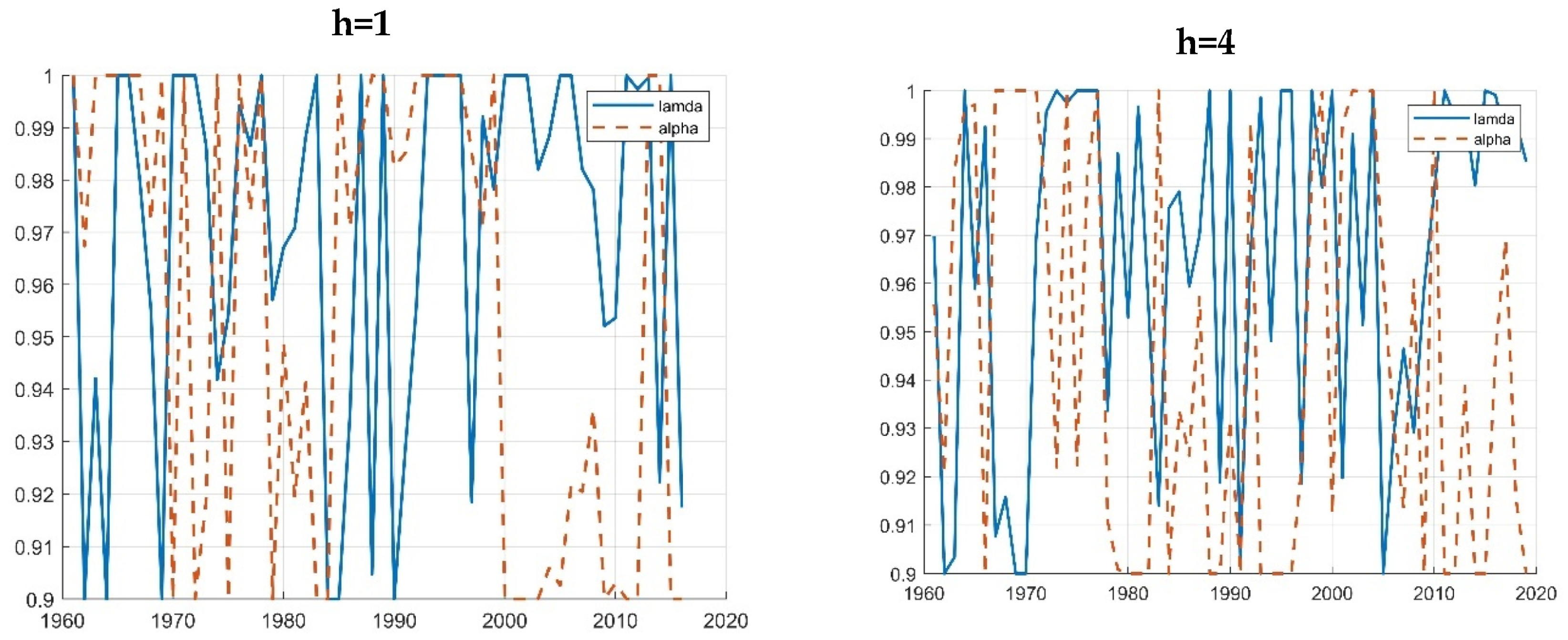
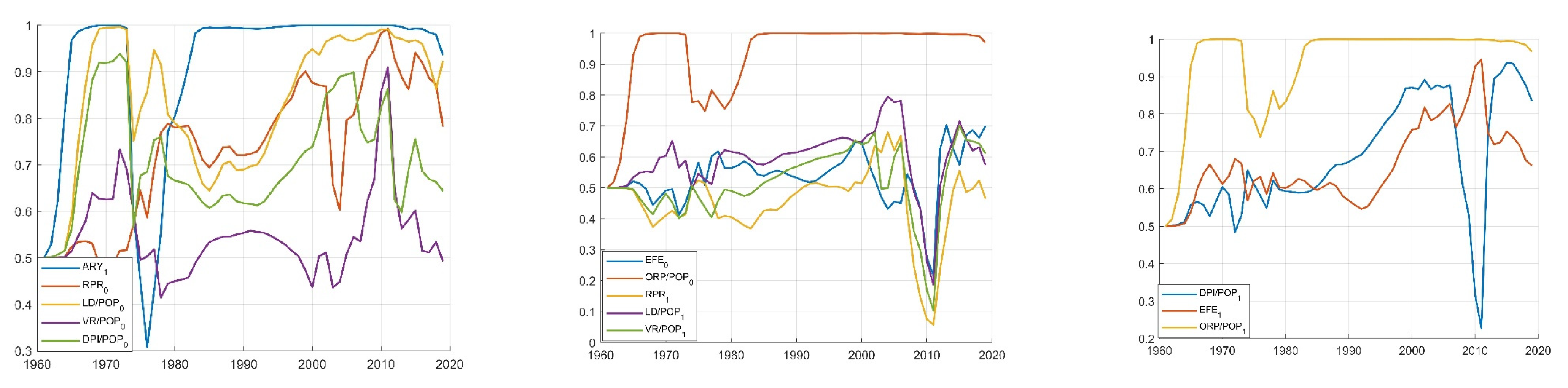
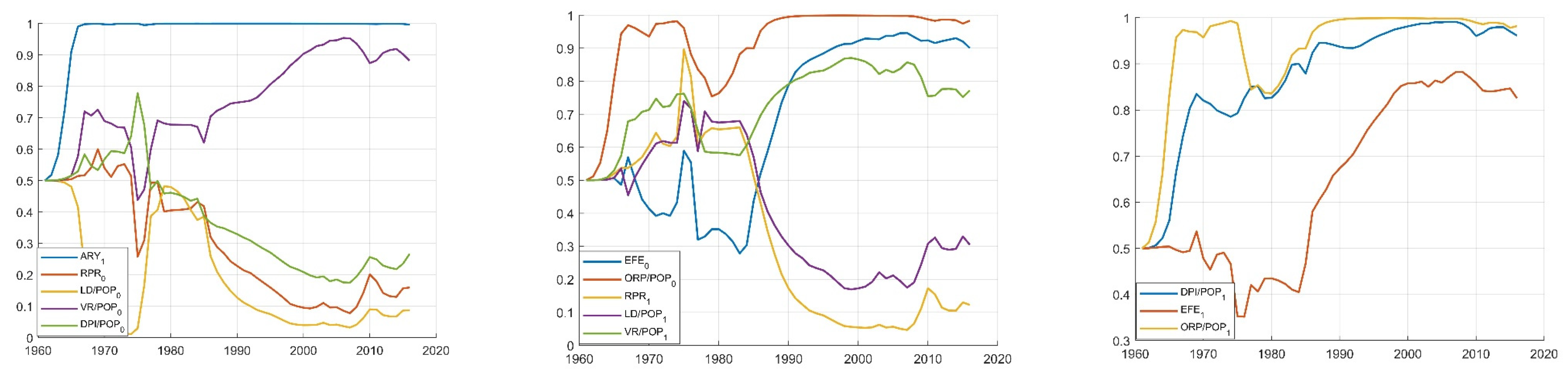
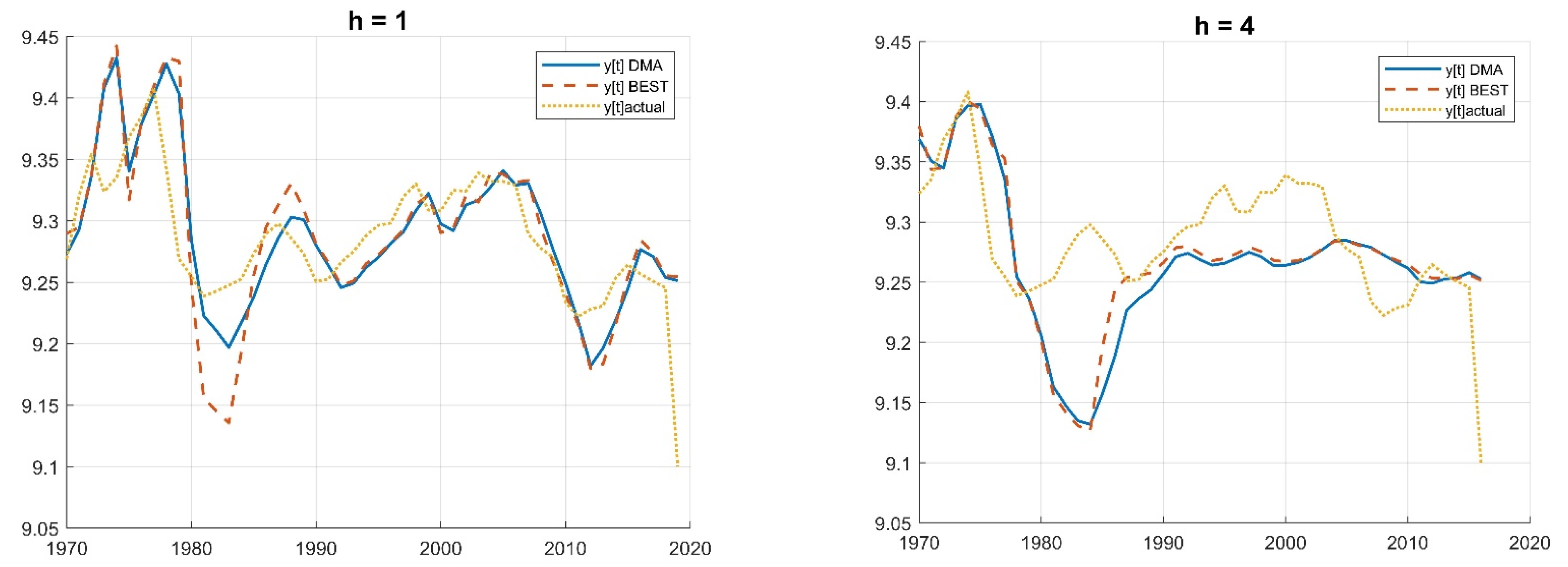
Annual observations for the United States from 1960 to 2020 were utilized in this analysis. Exogenous variables include measurements of demographic traits, economic activity, income, driving expenses, car pricing, and road availability. These variables in

Table 1. Research literature for estimating gasoline demand function to determine model variables.

Author	Type	Dep. Variable	Ind. Variable
Hughes et al. [33]	Time series OLS	Fuel demand/capita	Gas price
Wadud et al. [34]	RE panel (quarterly)	Fuel demand	Gas price
Rentziou et al. [35]	SURE panel model (annual)	State VMT	Gas price
Lin & Prince [36]	Dynamic times series	Fuel demand/capita	Gas price
Wang & Chen [37]	SEM (daily)	Household VMT	Gas price
Dillon et al. [38]	SEM (daily)	Household VMT	Gas price
Hymel & Small [39]	Simultaneous equations	State VMT	Fuel cost/mile
Levin et al. [40]	FE panel (daily/monthly)	Fuel demand/capita	Gas price
Dimitropoulos et al. [12]	Lit. review/meta-analysis	Fuel demand & VMT	Gas price
Taiebat et al. [41]	microeconomic model (daily)	Household VMT	Gas price
Gillingham [42]	Lit. review/Lit. survey	US VMT	gas price
Goetzke & Vance [11]	pooled OLS	Household VMT	Gas price
Chakraborty et al. [43]	OLS regression	TOT hh VMT	fuel cost (non-PEV)

are chosen based on an extensive review of the available literature.

Table 2. Variables and definitions.

Variable	Definition	Source
$\mathrm{G}\mathrm{U}/\mathrm{P}\mathrm{O}\mathrm{P}$	$\mathrm{G}\mathrm{U}/\mathrm{P}\mathrm{O}\mathrm{P}=\mathrm{l}\mathrm{n}(\frac{\mathrm{G}\mathrm{U}}{\mathrm{p}\mathrm{o}\mathrm{p}\mathrm{u}\mathrm{l}\mathrm{a}\mathrm{t}\mathrm{i}\mathrm{o}\mathrm{n}})$ $\mathrm{G}\mathrm{U}$ = Motor gasoline total end-use consumption	EIA
$\mathrm{D}\mathrm{P}\mathrm{I}/\mathrm{P}\mathrm{O}\mathrm{P}$	$\mathrm{D}\mathrm{P}\mathrm{I}/\mathrm{P}\mathrm{O}\mathrm{P}=\mathrm{l}\mathrm{n}(\frac{\mathrm{D}\mathrm{P}\mathrm{I}}{\mathrm{p}\mathrm{o}\mathrm{p}\mathrm{u}\mathrm{l}\mathrm{a}\mathrm{t}\mathrm{i}\mathrm{o}\mathrm{n}})$ $\mathrm{D}\mathrm{P}\mathrm{I}$ = Disposable personal income, Billions of Dollars	FRED
$\mathrm{R}\mathrm{P}\mathrm{R}$	$\mathrm{R}\mathrm{P}\mathrm{R}/\mathrm{P}\mathrm{O}\mathrm{P}=\mathrm{l}\mathrm{n}(\frac{\mathrm{R}\mathrm{P}\mathrm{R}}{\mathrm{p}\mathrm{o}\mathrm{p}\mathrm{u}\mathrm{l}\mathrm{a}\mathrm{t}\mathrm{i}\mathrm{o}\mathrm{n}})$ $\mathrm{R}\mathrm{P}\mathrm{R}$ = Unleaded Regular Gasoline, U.S. City Average Retail Price	EIA
$\mathrm{E}\mathrm{F}\mathrm{E}$	$\mathrm{E}\mathrm{F}\mathrm{E}=\mathrm{l}\mathrm{n}(\mathrm{F}\mathrm{E})$ $\mathrm{F}\mathrm{E}$ = All Motor Vehicles Fuel Efficiency (Miles per Gallon)	EIA
$\mathrm{L}\mathrm{D}/\mathrm{P}\mathrm{O}\mathrm{P}$	$\mathrm{L}\mathrm{D}/\mathrm{P}\mathrm{O}\mathrm{P}=\mathrm{l}\mathrm{n}(\frac{\mathrm{L}\mathrm{D}}{\mathrm{p}\mathrm{o}\mathrm{p}\mathrm{u}\mathrm{l}\mathrm{a}\mathrm{t}\mathrm{i}\mathrm{o}\mathrm{n}})$ $\mathrm{L}\mathrm{D}$ = Total Licensed Drivers	FHWA
$\mathrm{V}\mathrm{R}/\mathrm{P}\mathrm{O}\mathrm{P}$	$\mathrm{V}\mathrm{R}/\mathrm{P}\mathrm{O}\mathrm{P}=\mathrm{l}\mathrm{n}(\frac{\mathrm{V}\mathrm{R}}{\mathrm{p}\mathrm{o}\mathrm{p}\mathrm{u}\mathrm{l}\mathrm{a}\mathrm{t}\mathrm{i}\mathrm{o}\mathrm{n}})$ $\mathrm{V}\mathrm{R}$ = Total Motor Vehicle Registrations For All Motor Vehicles	FHWA
$\mathrm{O}\mathrm{R}\mathrm{P}/\mathrm{P}\mathrm{O}\mathrm{P}$	$\mathrm{O}\mathrm{R}\mathrm{P}/\mathrm{P}\mathrm{O}\mathrm{P}=\mathrm{l}\mathrm{n}(\frac{\mathrm{P}\mathrm{R}}{\mathrm{p}\mathrm{o}\mathrm{p}\mathrm{u}\mathrm{l}\mathrm{a}\mathrm{t}\mathrm{i}\mathrm{o}\mathrm{n}})$ $\mathrm{P}\mathrm{R}$ = Public Road Mileage	FHWA

FRED: Federal Reserve Economic Data; https://fred.stlouisfed.org, accessed on 20 June 2022; EIA: Energy Information Administration; https://www.eia.gov/, accessed on 20 June 2022; FHWA: Federal Highway Administration; https://highways.dot.gov/, accessed on 18 June 2022.

, below, provides a brief description of the variables included in our analysis, as well as a definition and reference to the source. Moreover, summary statistics for the variables that are used in the empirical analysis are presented in

Table 3. Descriptive statistics.

	Mean	Median	Maximum	Minimum	Std. Dev.
$\mathrm{G}\mathrm{U}/\mathrm{P}\mathrm{O}\mathrm{P}$	9.252	9.269	9.408	8.995	0.095
$\mathrm{D}\mathrm{P}\mathrm{I}/\mathrm{P}\mathrm{O}\mathrm{P}$	2.587	2.857	3.970	0.737	1.006
$\mathrm{R}\mathrm{P}\mathrm{R}$	0.048	0.152	1.293	−1.191	0.783
$\mathrm{E}\mathrm{F}\mathrm{E}$	2.708	2.797	2.901	2.477	0.158
$\mathrm{L}\mathrm{D}/\mathrm{P}\mathrm{O}\mathrm{P}$	−0.462	−0.401	−0.359	−0.727	0.112
$\mathrm{V}\mathrm{R}/\mathrm{P}\mathrm{O}\mathrm{P}$	−0.381	−0.290	−0.173	−0.889	0.208
$\mathrm{O}\mathrm{R}\mathrm{P}/\mathrm{P}\mathrm{O}\mathrm{P}$	9.655	9.655	9.888	9.453	0.142

.

4. Results

By comparing DMA predictions, we examine forecast performance. We attempted to empirically test several configurations of the ABC model to increase the accuracy of the forecast while achieving the quickest feasible computation speed. In conclusion, the number of bees was fixed at five, the greatest quantity of repetitions at five, and the lower and upper bound between 0.9% and 1%. Finally, we demonstrate the sensitivity of our findings to the choice of forgetting factors, $\mathsf{\alpha } \mathrm{a}\mathrm{n}\mathrm{d} \mathsf{\lambda }$. We provide findings for prediction horizons of one year (h = 1) and four years (h = 4). A prediction horizon of 4 means that we used the values of the independent variables in the previous 4 periods to predict the dependent variable in the current period. Obviously, with an increase in the prediction horizon, the prediction accuracy of the independent variables decreases. Our models all incorporate an intercept and a single lag between the dependent and independent variables. Experiments with lag lengths up to two revealed that a single lag produces the highest prediction results. Using the ABC approach, we sought to randomize the forgetting components in this study. Thus, our methodology not only provides for the automated determination of the two forgetting elements but also for their evolution over time to minimize the prediction model’s inaccuracy. These computations are carried out at a low computational cost. Thus, rather than selecting manually, we use a more precise selection mechanism. Figure 1 illustrates the outcome of estimating the components across time and the prediction horizons one and four. After estimating the model using the combined DMA-ABC model, the chance of each of the model’s independent variables being present is supplied. The posterior inclusion probability is shown in Figure 2 and Figure 3. That is, they quantify the likelihood that a predictor will help predict at time t. They are equivalent to the weights applied using DMA to models that incorporate a predictor. These graphs illustrate which predictors are significant at any given moment in time. These graphs demonstrate that DMS nearly always selects sparse models. These results are compelling evidence of model evolution. DMA has a significant theoretical advantage over other forecasting methodologies in that it enables the forecasting model to evolve. Of course, this gain may be negligible in a given empirical application if the forecasting model does not vary much over time. While the same trend remains true to a lesser degree, it is apparent that there is a significant change over time. That is, the forecasting model’s collection of predictors evolves with time. After 1980, practically all surface variables enter the model with varying probability. Intermittent values, of course, provide various outcomes. Between 2000 and 2015, the likelihood of existence, or the initial lag, of the majority of model variables is questioned. In comparison to other variables, vehicle registration has the lowest likelihood of being present, while public road mileage at the level and first log values indicate a high possibility of being included in gasoline demand forecasting.

Figure 4 illustrates the actual and predicted value of gasoline along with the forecast horizons h = 1 and h = 4. The accuracy of the model in estimating gasoline demand is seen in Figure 3. Additionally, expanding the prediction horizon resulted in a decline in the estimated model’s accuracy. Our earlier DMA and DMS findings were for our benchmark example, in which we used the ABC technique to determine a random forgetting factor that changes over time. As previously stated, researchers in this area use predetermined values for $\mathsf{\alpha } \mathrm{a}\mathrm{n}\mathrm{d} \mathsf{\lambda }$. As a consequence, Raftery et al. [17] used $\mathsf{\lambda }=\mathsf{\alpha }=0.99$ and suggest that the findings will remain resilient to accepting modifications in these variables. To test these claims of resilience, the results of our forecasting experiment utilizing different combinations of forgetting components are shown in

Table 4. Comparison of models.

Prediction Method	MAFE	MSFE	$\frac{\mathbf{M}\mathbf{A}\mathbf{F}\mathbf{E}}{{\mathbf{M}\mathbf{A}\mathbf{F}\mathbf{E}}_{\mathbf{B}}}$	$\frac{\mathbf{M}\mathbf{S}\mathbf{F}\mathbf{E}}{{\mathbf{M}\mathbf{S}\mathbf{F}\mathbf{E}}_{\mathbf{B}}}$		MAFE	MSFE	$\frac{\mathbf{M}\mathbf{A}\mathbf{F}\mathbf{E}}{{\mathbf{M}\mathbf{A}\mathbf{F}\mathbf{E}}_{\mathbf{B}}}$	$\frac{\mathbf{M}\mathbf{S}\mathbf{F}\mathbf{E}}{{\mathbf{M}\mathbf{S}\mathbf{F}\mathbf{E}}_{\mathbf{B}}}$
	h = 1					h = 4
DMA-ABC	0.55	3.60	1.01	0.98	DMA-ABC	0.71	4.86	0.96	0.96
DMS-ABC	0.47	3.02	0.86	0.82	DMS-ABC	0.58	3.87	0.78	0.76
DMA $\mathsf{\lambda }$ = 0.9662; $\mathsf{\alpha }$ = 0.9449	0.53	3.60	0.98	0.98	DMA $\mathsf{\lambda }$ = 0.9698; $\mathsf{\alpha }$ = 0.9556	0.71	4.85	0.95	0.96
DMS $\mathsf{\lambda }$ = 0.9662; $\mathsf{\alpha }$ = 0.9449	0.44	3.00	0.81	0.81	DMS $\mathsf{\lambda }$ = 0.9698; $\mathsf{\alpha }$ = 0.9556	0.58	3.87	0.78	0.76
DMA $\mathsf{\lambda }$ = $\mathsf{\alpha }$ = 0.99	0.54	3.65	0.99	0.99	DMA $\mathsf{\lambda }$ = $\mathsf{\alpha }$ = 0.99	0.73	5.03	0.98	0.99
DMS $\mathsf{\lambda }$ = $\mathsf{\alpha }$ = 0.99	0.45	3.04	0.82	0.83	DMS $\mathsf{\lambda }$ = $\mathsf{\alpha }$ = 0.99	0.60	3.98	0.80	0.79
DMA $\mathsf{\lambda }$ = $\mathsf{\alpha }$ = 0.95	0.55	3.57	1.01	0.97	DMA $\mathsf{\lambda }$ = $\mathsf{\alpha }$ = 0.95	0.72	4.98	0.97	0.98
DMS $\mathsf{\lambda }$ = $\mathsf{\alpha }$ = 0.95	0.46	2.99	0.85	0.81	DMS $\mathsf{\lambda }$ = $\mathsf{\alpha }$ = 0.95	0.60	3.98	0.80	0.79
DMA $\mathsf{\lambda }$ = 0.95; $\mathsf{\alpha }$ = 0.99	0.55	3.56	1.01	0.97	DMA $\mathsf{\lambda }$ = 0.95; $\mathsf{\alpha }$ = 0.99	0.72	4.95	0.97	0.98
DMS $\mathsf{\lambda }$ = 0.95; $\mathsf{\alpha }$ = 0.99	0.46	2.99	0.85	0.81	DMS $\mathsf{\lambda }$ = 0.95; $\mathsf{\alpha }$ = 0.99	0.60	3.93	0.80	0.78
DMA $\mathsf{\lambda }$ = 0.99; $\mathsf{\alpha }$ = 0.95	0.54	3.66	0.99	1.00	DMA $\mathsf{\lambda }$ = 0.99; $\mathsf{\alpha }$ = 0.95	0.74	5.04	0.99	0.99
DMS $\mathsf{\lambda }$ = 0.99; $\mathsf{\alpha }$ = 0.95	0.45	3.04	0.82	0.83	DMS $\mathsf{\lambda }$ = 0.99; $\mathsf{\alpha }$ = 0.95	0.60	3.98	0.80	0.79
TVP- BMA ($\mathsf{\lambda }$ = 1)	0.55	3.68	1.00	1.00	TVP- BMA ($\mathsf{\lambda }$ = 1)	0.75	5.08	1.00	1.00
BMA ($\mathsf{\lambda }$ = $\mathsf{\alpha }$ = 1)	0.54	3.68	1.00	1.00	BMA ($\mathsf{\lambda }$ = $\mathsf{\alpha }$ = 1)	0.75	5.07	1.00	1.00

. MSFE and MAFE values for various models of DMA-ABC, DMS-ABC, DMS, DMA, BMA, TVP-BMA, and TVP are provided in Table 4 for prediction horizons 1 and 4. The results of the comparison of several models in Table 4 indicate that the combined model of DMS and ABC, with the option of automatically acquiring forgetting factors over time, obtains the greatest results in forecasting gasoline demand. According to the DMA-ABC model, the mean values of the forgetting components are equal to $\mathsf{\alpha }$ = 0.9449 and $\mathsf{\lambda }$ = 0.9662. Even taking the constant mean values of computational forgetting factors into account produced satisfactory results. It is noteworthy that the value $\mathsf{\alpha }$ = 0.9449 enables relatively fast model evolution over time. This is similar to a previous tale we mentioned: it seems that allowing models to evolve is more significant than allowing parameters to vary with $\mathsf{\lambda }$ = 0.9662 for increasing forecast performance. The BME model (with λ = α = 1) does not have any dynamic approach, which means that while the estimated coefficients are constant over time, the input variables to the model are also constant over time. To investigate the effects of adding dynamics to the model in increasing the forecasting accuracy, we added two more columns to Table 4. In these two columns, the ratio of MAFE and MSFE of different models is calculated with the MAFE and MSFE values of the BMA model (with B index). Based on the results, the prediction error values in model DMS-ABC are about 0.82 of the prediction error in model BMA with a prediction horizon of 1. In addition, this value is equal to 0.76 in the forecast horizon of 4. Therefore, by increasing the prediction horizon, moving towards dynamic models leads to a further increase in prediction accuracy.

5. Conclusions and Implications

Accurate modeling and forecasting of gasoline demand may provide a valuable framework for policymakers to consider the policy implications of their energy market activities, which is the goal of this study. The primary shortcoming in prior forecasting models was their inability to accurately predict over time. Policymakers, on the other hand, should disregard short-term and temporary variations in gasoline demand in favor of economic stability. Therefore, the objective of this study was to develop a nonlinear dynamic model DMA-ABS to forecast gasoline consumption in the United States using annual data from 1960 to 2020. These models may be used to determine changes in both the input variables and the parameters of variables through time. The inclusion of two forgetting variables in the DMA model may be used to control the speed of such dynamics in the model, which has been previously determined manually in earlier research. In this work, we sought to implement a random process of forgetting factor selection using the ABC method. Therefore, one of the primary objectives of this study is to merge ABC with DMA to increase prediction accuracy. The findings of the DMS estimation model indicated that the input variables fluctuate with time, emphasizing the need of employing dynamic models rather than constant input variables for estimating gasoline demand.

Gasoline demand prediction helps policymakers to make informed decisions on issues related to energy security, environmental regulations, and transportation infrastructure. For instance, it can assist in determining the number of gas stations required to meet demand in a particular area, the type of fuel to be used in different transportation modes, and the amount of investment needed to maintain or upgrade the transportation infrastructure. Moreover, gasoline demand prediction can aid in managing the price of gasoline. It helps in determining the price level that will meet the demand and supply equilibrium. Therefore, it is recommended that in future research, the DMA model will be integrated with other evolutionary algorithms, such as particle swarm optimization (PSO), genetic algorithm (GA), etc., to compare the results and provide a more accurate prediction of the gasoline market through the expansion of the model presented in this research.

References

1. EIA. Annual Energy Outlook (AEO) Retrospective Review: Evaluation of AEO 2020 and Previous Reference Case Projections. Anal. Proj. U.S. Energy Inf. Adm. 2020, 92010, 1–15. [Google Scholar]
2. McCarthy, P.S. Market Price and Income Elasticities of New Vehicle Demands. Rev. Econ. Stat. 1996, 78, 543. [Google Scholar] [CrossRef]
3. Shen, C.; Linn, J. The Effect of Income on Vehicle Demand: Evidence from China’S New Vehicle Market; Resources for the Future: Washington, DC, USA, 2021. [Google Scholar]
4. Dargay, J.; Gately, D.; Sommer, M. Vehicle ownership and income growth, worldwide: 1960–2030. Energy J. 2007, 28, 143–170. [Google Scholar] [CrossRef] [Green Version]
5. Huo, H.; Wang, M. Modeling Future Vehicle Sales and Stock in China. Energy Policy 2012, 43, 17–29. [Google Scholar] [CrossRef]
6. Oladosu, G. An Almost Ideal Demand System Model of Household Vehicle Fuel Expenditure Allocation in the United States. Energy J. 2003, 24, 1–21. [Google Scholar] [CrossRef]
7. Kim, Y.; Kim, S. Forecasting Charging Demand of Electric Vehicles Using Time-Series Models. Energies 2021, 14, 1487. [Google Scholar] [CrossRef]
8. Fouquet, R. Trends in Income and Price Elasticities of Transport Demand (1850-2010). Energy Policy 2012, 50, 62–71. [Google Scholar] [CrossRef] [Green Version]
9. Graham, D.J.; Glaister, S. Road Traffic Demand Elasticity Estimates: A Review. Transp. Rev. 2004, 24, 261–274. [Google Scholar] [CrossRef]
10. Bento, A.M.; Goulder, L.H.; Jacobsen, M.R.; Von Haefen, R.H. Distributional and Efficiency Impacts of Increased US Gasoline Taxes. Am. Econ. Rev. 2009, 99, 667–699. [Google Scholar] [CrossRef] [Green Version]
11. Goetzke, F.; Vance, C. An Increasing Gasoline Price Elasticity in the United States? Energy Econ. 2021, 95, 104982. [Google Scholar] [CrossRef]
12. Dimitropoulos, A.; Oueslati, W.; Sintek, C. The Rebound Effect in Road Transport: A Meta-Analysis of Empirical Studies. Energy Econ. 2018, 75, 163–179. [Google Scholar] [CrossRef]
13. Ghysels, E.; Plazzi, A.; Valkanov, R.; Torous, W. Forecasting Real Estate Prices. Handb. Econ. Forecast. 2013, 2, 509–580. [Google Scholar] [CrossRef]
14. Plakandaras, V.; Gupta, R.; Gogas, P.; Papadimitriou, T. Forecasting the U.S. Real House Price Index. Econ. Model. 2015, 45, 259–267. [Google Scholar] [CrossRef] [Green Version]
15. Próchniak, M.; Witkowski, B. Time Stability of the Beta Convergence among EU Countries: Bayesian Model Averaging Perspective. Econ. Model. 2013, 30, 322–333. [Google Scholar] [CrossRef]
16. Man, G. Competition and the Growth of Nations: International Evidence from Bayesian Model Averaging. Econ. Model. 2015, 51, 491–501. [Google Scholar] [CrossRef]
17. Raftery, A.E.; Kárný, M.; Ettler, P. Online Prediction under Model Uncertainty via Dynamic Model Averaging: Application to a Cold Rolling Mill. Technometrics 2010, 52, 52–66. [Google Scholar] [CrossRef] [Green Version]
18. Koop, G.; Korobilis, D. Forecasting Inflation Using Dynamic Model Averaging. Int. Econ. Rev. 2012, 53, 867–886. [Google Scholar] [CrossRef] [Green Version]
19. Koop, G.; Korobilis, D. UK Macroeconomic Forecasting with Many Predictors: Which Models Forecast Best and When Do They Do So? Econ. Model. 2011, 28, 2307–2318. [Google Scholar] [CrossRef] [Green Version]
20. Del Negro, M.; Primiceri, G.E. Time Varying Structural Vector Autoregressions and Monetary Policy: A Corrigendum. Rev. Econ. Stud. 2010, 82, 1342–1345. [Google Scholar] [CrossRef] [Green Version]
21. Pesaran, M.H.; Timmermann, A. A Recursive Modelling Approach to Predicting UK Stock Returns. Econ. J. 2000, 110, 159–191. [Google Scholar] [CrossRef]
22. Bork, L.; Møller, S.V. Forecasting House Prices in the 50 States Using Dynamic Model Averaging and Dynamic Model Selection. Int. J. Forecast. 2015, 31, 63–78. [Google Scholar] [CrossRef]
23. Wei, Y.; Cao, Y. Forecasting House Prices Using Dynamic Model Averaging Approach: Evidence from China. Econ. Model. 2017, 61, 147–155. [Google Scholar] [CrossRef]
24. Dong, X.; Yoon, S.M. What Global Economic Factors Drive Emerging Asian Stock Market Returns? Evidence from a Dynamic Model Averaging Approach. Econ. Model. 2019, 77, 204–215. [Google Scholar] [CrossRef]
25. Naser, H.; Alaali, F. Can Oil Prices Help Predict US Stock Market Returns? Evidence Using a Dynamic Model Averaging (DMA) Approach. Empir. Econ. 2018, 55, 1757–1777. [Google Scholar] [CrossRef]
26. Drachal, K. Forecasting Spot Oil Price in a Dynamic Model Averaging Framework—Have the Determinants Changed over Time? Energy Econ. 2016, 60, 35–46. [Google Scholar] [CrossRef]
27. Byrne, J.P.; Cao, S.; Korobilis, D. Forecasting the Term Structure of Government Bond Yields in Unstable Environments. J. Empir. Financ. 2017, 44, 209–225. [Google Scholar] [CrossRef] [Green Version]
28. Beckmann, J.; Koop, G.; Korobilis, D.; Schüssler, R.A. Exchange Rate Predictability and Dynamic Bayesian Learning. J. Appl. Econom. 2020, 35, 410–421. [Google Scholar] [CrossRef] [Green Version]
29. Byrne, J.P.; Korobilis, D.; Ribeiro, P.J. On the Sources of Uncertainty in Exchange Rate Predictability. Int. Econ. Rev. 2018, 59, 329–357. [Google Scholar] [CrossRef] [Green Version]
30. Ma, F.; Liu, J.; Wahab, M.I.M.; Zhang, Y. Forecasting the Aggregate Oil Price Volatility in a Data-Rich Environment. Econ. Model. 2018, 72, 320–332. [Google Scholar] [CrossRef]
31. Avramov, D. Stock Return Predictability and Model Uncertainty. J. Financ. Econ. 2002, 64, 423–458. [Google Scholar] [CrossRef]
32. Koop, G.; Potter, S. Forecasting in Dynamic Factor Models Using Bayesian Model Averaging. Econom. J. 2004, 7, 550–565. [Google Scholar] [CrossRef] [Green Version]
33. Hughes, J.E.; Knittel, C.R.; Sperling, D. Evidence of a Shift in the Short-Run Price Elasticity of Gasoline Demand. Energy J. 2008, 29, 113–134. [Google Scholar] [CrossRef] [Green Version]
34. Wadud, Z.; Graham, D.J.; Noland, R.B. Gasoline Demand with Heterogeneity in Household Responses. Energy J. 2010, 31, 47–74. [Google Scholar] [CrossRef] [Green Version]
35. Rentziou, A.; Gkritza, K.; Souleyrette, R.R. VMT, Energy Consumption, and GHG Emissions Forecasting for Passenger Transportation. Transp. Res. Part A Policy Pract. 2012, 46, 487–500. [Google Scholar] [CrossRef]
36. Lin, C.Y.C.; Prince, L. Gasoline Price Volatility and the Elasticity of Demand for Gasoline. Energy Econ. 2013, 38, 111–117. [Google Scholar] [CrossRef]
37. Wang, T.; Chen, C. Impact of Fuel Price on Vehicle Miles Traveled (VMT): Do the Poor Respond in the Same Way as the Rich? Transportation (Amst) 2014, 41, 91–105. [Google Scholar] [CrossRef]
38. Dillon, H.S.; Saphores, J.D.; Boarnet, M.G. The Impact of Urban Form and Gasoline Prices on Vehicle Usage: Evidence from the 2009 National Household Travel Survey. Res. Transp. Econ. 2015, 52, 23–33. [Google Scholar] [CrossRef]
39. Hymel, K.M.; Small, K.A. The Rebound Effect for Automobile Travel: Asymmetric Response to Price Changes and Novel Features of the 2000s. Energy Econ. 2015, 49, 93–103. [Google Scholar] [CrossRef] [Green Version]
40. Levin, L.; Lewis, M.S.; Wolak, F.A. High Frequency Evidence on the Demand for Gasoline. Am. Econ. J. Econ. Policy 2017, 9, 314–347. [Google Scholar] [CrossRef] [Green Version]
41. Taiebat, M.; Stolper, S.; Xu, M. Corrigendum to “Forecasting the Impact of Connected and Automated Vehicles on Energy Use: A Microeconomic Study of Induced Travel and Energy Rebound”. Appl. Energy 2019, 256, 297–308. [Google Scholar] [CrossRef] [Green Version]
42. Gillingham, K.T. The rebound effect and the proposed rollback of U.S. fuel economy standards. Rev. Environ. Econ. Policy 2020, 14, 136–142. [Google Scholar] [CrossRef]
43. Chakraborty, D.; Hardman, S.; Tal, G. Integrating plug-in electric vehicles (PEVs) into household fleets-factors influencing miles traveled by PEV owners in California. Travel Behav. Soc. 2022, 26, 67–83. [Google Scholar] [CrossRef]
Figure 1. α and λ over time (h = 1, h = 4).
Energies 16 04795 g001
Figure 2. Posterior probability (h = 1).
Energies 16 04795 g002
Figure 3. Posterior probability (h = 4).
Energies 16 04795 g003
Figure 4. The actual and predicted value of gasoline demand in the forecast horizon h = 1 and h = 4 α = 0.9449; λ.
Energies 16 04795 g004