Analysis of the Effects of Different Nanofluids on Critical Heat Flux Using Artificial Intelligence

Abstract

Nanofluid (NF) pool boiling experiments have been conducted widely in the past two decades to study and understand how nanoparticles (NP) affect boiling heat transfer and critical heat flux (CHF). However, the physical mechanisms related to the improvements in CHF in NF pool boiling are still not conclusive due to the coupling effects of the surface characteristics and the complexity of the experimental data. In addition, the current models for pool boiling CHF prediction, which consider surface microstructure characteristics, show limited agreement with the experimental data and do not represent NF pool boiling CHF. In this scenario, artificial intelligence tools, such as machine learning (ML) regressor models, are a very promising means of solving this nonlinear problem. This study focuses on creating a new model to provide more accurate NF pool boiling CHF predictions based on pressure, substrate thermal effusivity, and NP size, concentration, and effusivity. Three ML models (supporting vector regressor—SVR, multi-layer perceptron—MLP, and random forest—RF) were constructed and showed good agreement with an experimental database built from the literature, with MLP presenting the highest mean R² score and the lowest variability. A systematic methodology for optimizing the ML models is proposed in this work.

1. Introduction

In the past 20 years, extensive studies of critical heat flux (CHF) enhancement in pool boiling have been carried out using nanofluids (NFs), which are a mixture of nanoparticles (NPs) and conventional fluids. CHF is defined as the maximum allowable heat flux from a heated surface to the liquid/vapor mixture in two-phase flow systems. Enhanced CHF allows for higher heat flux margins and higher thermal performance in boilers, electronic device coolers, heat exchangers, and nuclear reactors. In particular, it could allow cladding temperatures in advanced nuclear water-cooled reactors to reach higher temperature and heat flux limits. Following You et al.’s investigation in 2003 [1], many experimental studies [2,3,4,5,6,7,8,9,10,11,12,13,14,15,16,17,18,19,20,21,22,23,24,25,26,27,28,29,30,31,32,33,34,35,36,37,38,39,40,41,42,43,44] applied different NPs, using different deposition methods and surface materials, and evaluated the CHF changes. According to these studies, NPs are deposited on the surface microstructure, which modifies parameters such as roughness, wettability, and wickability, delaying the CHF occurrence to higher heat fluxes under certain conditions.

Although the surface microstructure modifications due to NP deposition are usually well characterized using post-process imaging, the physical mechanistic process itself and the importance quantification of each independent parameter in NF pool boiling CHF still need to be better understood. Several CHF correlations were investigated by Liang and Mudawar [45] following the initial work by Kutateladze [46]. These correlations account for surface characteristics, as can be seen in the work by Kandlikar [47]. However, these correlations are limited by surface microstructure characteristics and do not account for the NF properties.

The coupled impact of the surface with NF characteristics is very complex and creates a broad area for investigation. As the CHF and NF parameters do not have a linear relationship, machine learning (ML) can be a suitable tool with which to evaluate each parameter’s importance to CHF as well as their combined impact. ML proved to be a very good tool with which to solve non-linear CHF and boiling problems and has been applied to several heat transfer problems in the past few years [48,49,50].

Based on the above discussion, this study proposes a systematic methodology for the development of ML models to fill the gap left by the empirical investigations. The ML models were developed to predict the CHF values in NF pool boiling for a wide range of conditions using a database built from the open literature. These models were also used to evaluate the importance of each intrinsic parameter (i.e., pressure, substrate thermal effusivity, and NP thermal effusivity, size, and concentration) in NF pool boiling CHF.

Three different ML models were developed: support vector regressor (SVR), multi-layer perceptron (MLP), and random forest (RF), using a water-based NF pool boiling CHF database, which will be discussed in the following sections.

2. Database Construction

A CHF database was constructed by collecting information from different water-based NF pool boiling experiments, as shown in

Table 1. Experimental studies used for data collection.

Author (s)	Pressure (kPa)	Heating Element	Nanoparticle	NP Average Size (nm)	NF Concentration (vol.%)	Number of Datapoints
Kim et al. [2]	101.33	NiCr wire	TiO2	85	0.0001–0.1	5
Kim et al. [3] +	101.33	316 SS wire	Al2O3 ZrO2 SiO2	160 180 30	0.001–0.1	9
Stange et al. [5] #	98.16	316 SS wire Zr wire	TiO2 Al2O3 ZrO2 YSZ	7–250 15–60 20–45 25	0.000249–0.0249	16
Kumar et al. [13]	97.66	NiCr wire	Al2O3	10	0.01–0.05	4
Kshirsagar and Shrivastava [15] #	94.61	NiCr wire	Al2O3	30	0.076–0.382	5
Yao et al. [17] #	70.00–130.00	Copper plate	Al2O3	30–50	0.0025	4
Lee et al. [19] + #	100.46–1100.00	NiCr wire	Al2O3 Fe3O4	25	0.0001	6
Ciloglu [21]	83.00	Copper block	SiO2	20	0.01–0.1	3
Sulaiman et al. [22] #	100.40	Copper plate	TiO2 Al2O3 SiO2	21 13 20	0.00094–0.0252	16
Reddy and Venkatachalapathy [23]	100.27	Copper plate	Al2O3	50	0.01–0.03	2
Ham et al. [24]	3.00	Copper plate	Al2O3	50	0.001–0.1	8
Lee et al. [25] + #	100.46	NiCr wire	Fe3O4 Al2O3 TiO2	25 60 15	0.0001–0.01	11
Bang and Chang [26]	100.46	Copper plate	Al2O3	47	0.5–4.0	4
Song et al. [27]	100.46	304 SS plate	SiC	100	0.0001–0.01	6
Rostamian and Etesami [29]	83.80	Copper surface	SiO2	10	0.005–0.01	3
Vasquez and Kumar [30]	100.92	NiCr ribbon	SiO2	10	0.1–2.0	8
Golubovic et al. [31] #	99.16	NiCr wire	Al2O3	22.6–46	0.000015–0.0002	13
Jung et al. [32]	96.30	Copper wire	TiO2	85.3	0.000001–0.1	6
Jung et al. [33]	4.00	NiCr wire	Al2O3	45	0.00001–0.1	5
Dadjoo et al. [35]	84.60	Copper	SiO2	10.5	0.001–0.005	3
Kathiravan et al. [36] *	98.26	Stainless Steel	Cu	10	0.028–0.113	3
Hedge et al. [37]	101.33	NiCr wire	Al2O3	45	0.01–0.09	5
Kim et al. [38]	4.00	NiCr wire	Al2O3	45	0.00001–0.1	5
Shahmoradi et al. [39]	84.60	Copper plate	Al2O3	40	0.001–0.1	5
Kathiravan et al. [40] *	98.26	Stainless Steel	Cu	15	0.028–0.113	3
Hu et al. [41] #	99.61	Platinum	SiO2	100	0.00034–0.0013	3
Salari et al. [42] #	101.33	Copper	TiO2	45	0.00025–0.00075	3
Ahn and Kim [43]	97.90	Copper plate	Al2O3	47	0.001	1
Yang and Liu [44] #	7.4–103.00	Copper	SiO2	30	0.00627	3

* Stainless steel type was not specified; thus, 316 L stainless steel properties were used. + NP average size was not provided, then the mean value of the nanoparticle size range was used. # Nanofluid concentration unit was converted to vol.%.

. The data collected include sets with five main features: (1) substrate thermal effusivity; (2) system pressure; (3) NP thermal effusivity; (4) NP size; and (5) NF concentration. Among those features, the last three were selected because they represent the NF characteristics and encompass the main purpose of this study. Furthermore, according to many NF-related studies, those features highly affect CHF, as will be discussed in the following sections. Substrate thermal effusivity was selected to investigate the ways in which different substrates affect NF pool boiling and whether there is a relationship between the substrate and the different nanoparticles. Finally, the pressure was selected as a feature because it is known to highly affect CHF in water-based pool boiling experiments.

In total, the built database accounted for 170 NF pool boiling CHF datapoints, with the pressure ranging from 3 to 1000 kPa, NP size ranging from 7 to 250 nm, and NF concentration ranging from 10⁻⁶ to 4 vol.%. The substrate and NP thermal effusivities were determined using material properties; hence, they were specific for each material. The substrate materials included nichrome, stainless steel, copper, zirconium, and platinum. The NP types included alumina (Al₂O₃), silica (SiO₂), titania (TiO₂), zirconia (ZrO₂), copper (Cu), yttria-stabilized zirconia (YSZ), silicon carbide (SiC), and magnetite (Fe₃O₄).

Database Assumptions and Limitations

The data collection was challenging because different authors present their data in their own manner. For example, some of them highlighted the CHF points on the plots, while others mentioned them in texts or tables. In addition, despite the fact that they highly affect CHF, surface microstructure features such as roughness and contact angles were only presented in a small number of studies. Therefore, these parameters are briefly discussed separately in Section 5.5, but they are not included in the ML models due to the lack of sufficient information. The effective boiling areas of the different substrates were also not easy to determine due to the lack of heating element dimensions in most of the investigations. The precoated surface data were also not considered because their boiling dynamics differed from those of bare surface NFs; therefore, the ML models would not be able to make predictions based on the available information.

Fluid temperature or subcooling was also not taken into account since these experimental investigations only considered the liquid at the saturated temperature, i.e., zero subcooling. Two important restrictions for the collected data included the horizontal orientation of the substrate surfaces, which only faced upward, and the fact that only water-based NF pool boiling experiments were conducted.

Substrate orientation [26,28] and non-water-based NF [12,14,32,33,34] are very interesting topics to be discussed in a further study; however, they were considered to be outside of the scope of this study.

The thermal effusivity is determined using material properties. It is defined as the material’s energy transfer capacity with its surrounding environment, and it is calculated according to Equation (1):

$${\epsilon }_{th}=\sqrt{k\rho c_p}$$

(1)

where $k$ is the thermal conductivity, $\rho$ is the density, and $c_p$ is the heat capacity. When these properties were given in an uncertain range, the mean value was selected. The same procedure was used for the NP size [3,19,25], as described in the Table 1 footnotes.

Two further important assumptions were used for the database construction: the NF concentration unit was converted to vol.% [5,15,17,19,22,25,31,41,42,44], and 316 L stainless steel properties were used for the non-specified stainless steel heating elements [36,40].

3. Methodology: Machine Learning Models

In order to analyze and make a valuable comparison, three different machine learning (ML) models were implemented into a database composed of CHF values for different nanofluids using Sklearn toolkit with Python. Those models were selected due to their capacity to fit non-linear problems, which is the case with CHF and its related features analyzed in this study. A brief explanation of these models is presented in this section to clarify the hyperparameter optimization in the model construction.

3.1. Support Vector Regressor (SVR)

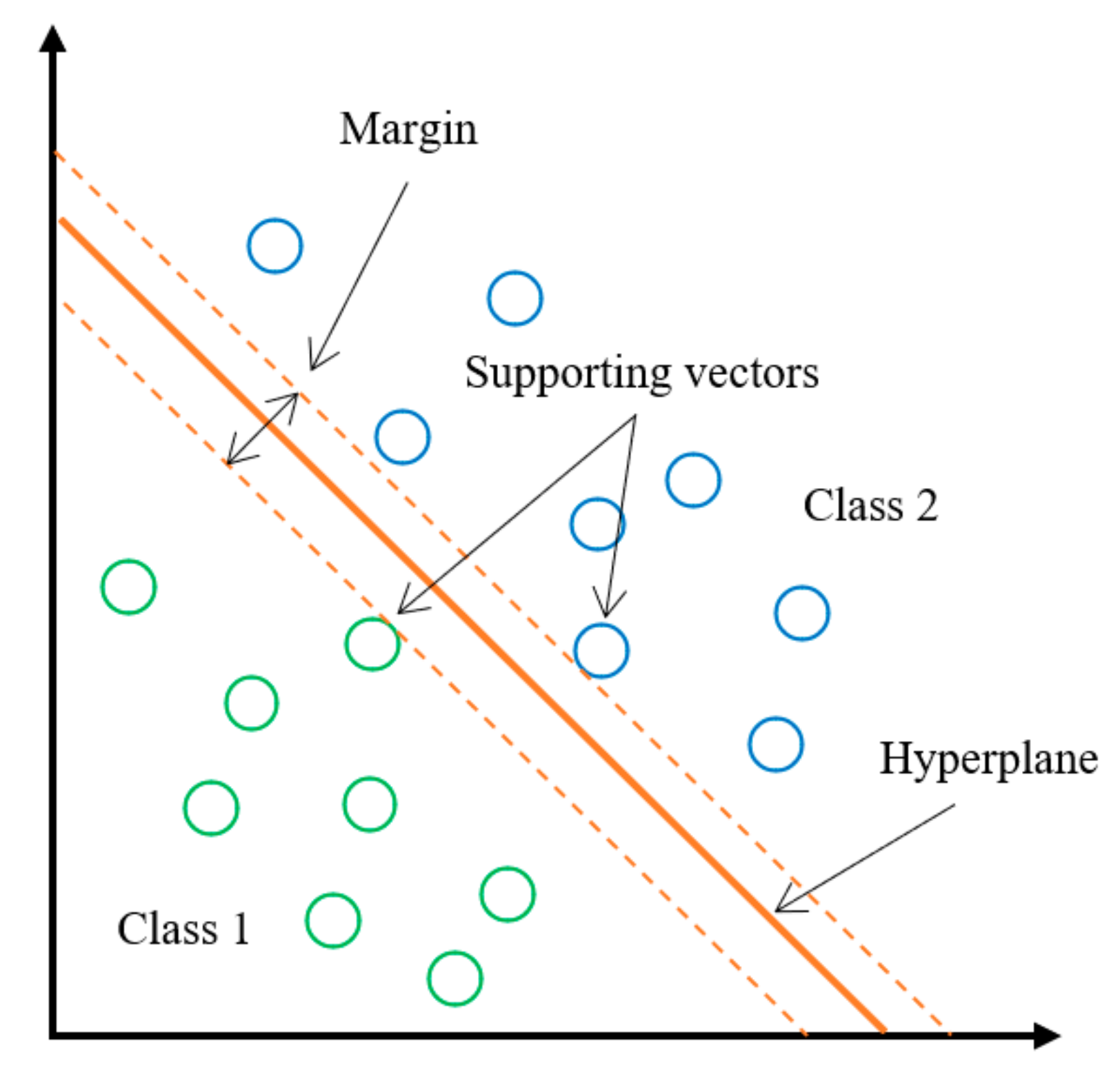
Support vector regressor (SVR) is one of the most popular regression models in ML because it can correctly predict non-linear problems. This model is an application of the support vector machine (SVM), which is a supervised learning classification algorithm. SVM is applied to a dataset to separate it into different classes. The datapoints are separated by a hyperplane, as shown in Figure 1. Because many hyperplanes could be generated to classify the data, only the best hyperplane is selected. The two closest hyperplane datapoints are defined as supporting vectors, and the distance between them is defined as the margin. The best hyperplane will be the one that optimizes the margin.

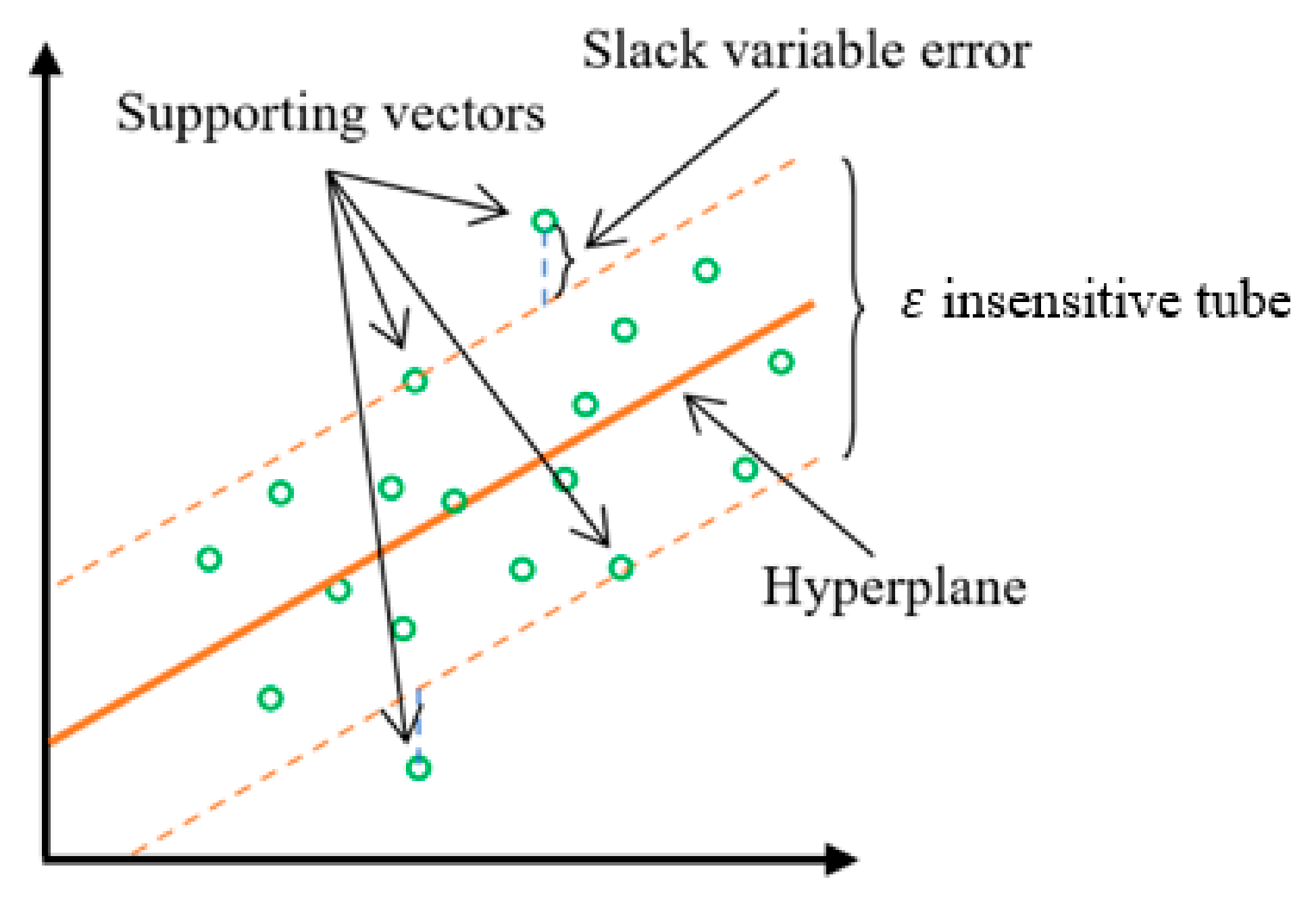
In Figure 1, the hyperplane is a line since it is a 2D representation. In a 3D case, the hyperplane would be a plane, and so on. The SVR uses a very similar concept of regression methods. However, instead of using a hyperplane to classify the data, it fits the best hyperplane to the dataset. The SVR fits the best insensitive tube ($\epsilon )$ that envelops most of the datapoints. The points inside the tube are not used for error calculation since they are within the tolerance level (margin). This tube is optimized by minimizing the error of the slack variables (datapoints outside the tube). In SVR, the supporting vectors will be the datapoints outside the tube and on its boundaries, as shown in Figure 2.

The SVR hyperparameters optimized prior to the dataset analysis were: (1) kernel, which is the function used in the algorithm to transform (mapping) the data into a higher dimension; (2) C value, which is proportional to the inverse of the regularization parameter and balances the importance of the slack variable errors in the models’ optimization; (3) gamma, which is a coefficient associated with three kernel functions, radial basis function (RBF), sigmoid, and polynomial; and (4) $\epsilon$, which specifies the insensitive tube margin thickness. The hyperparameter optimization results are discussed in Section 4 prior to each ML model implementation.

3.2. Multi-Layer Perceptron (MLP)

The multi-layer perceptron (MLP) is a feedforward artificial neural network (ANN) model characterized by having more than one intermediate layer, known as the hidden layer. In an ANN, random weights and biases are initialized and used by the neurons to generate an output (y). The obtained output is then compared to the real output and the weights ($w_{ij}^k)$ and biases (b_k) are updated accordingly. A representation of the MLP is shown in Figure 3.

Each arrow connecting the input parameters to the neurons and connecting each neuron to the next neuron has a different weight. Because there are too many connections, the weight indexes must be carefully stored and accounted for. Every neuron has an internal activation function that is applied to the input parameters entering a neuron, which transforms a linear combination into a nonlinear output. For a non-linear analysis, the activation function must be non-linear. In Figure 3, it can be observed that the larger the number of neurons and hidden layers the more complex is the ANN. Finally, a solver is used to build the ANN model, which is the mathematical approach used for the backward updates of the weights and biases.

The MLP hyperparameters optimized prior to the dataset analysis were: (1) the number of hidden layers; (2) the number of neurons in each layer; (3) the activation function of each hidden layer; and (4) the optimization solver.

3.3. Random Forest (RF)

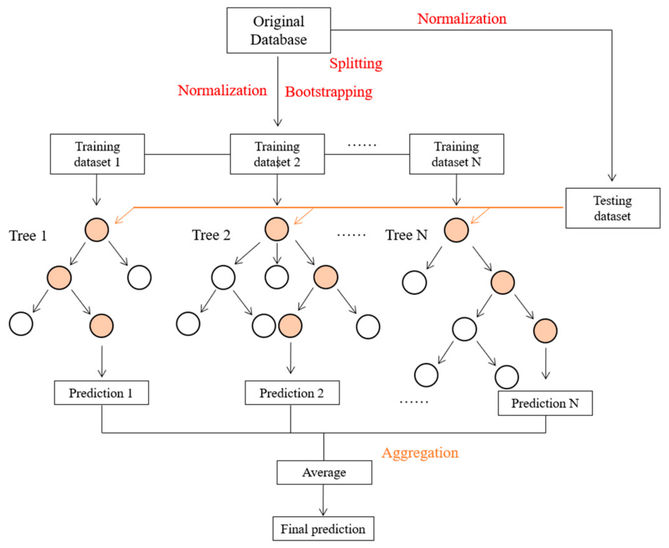
RF has proven to be a powerful tool for solving non-linear problems. The term random comes from the fact that it generates a set of different decision trees. These trees are all different because they are generated by two random processes, bootstrapping and random feature selection, generating different outputs and presenting different structures (nodes, branches, and leaves). The reason for the term forest is because it generates a set of decision trees; it is much less sensitive to the training data than a single decision tree, Figure 4.

The RF model implements bootstrapping and random feature selection, two random processes. Bootstrapping implements more randomness in the trees’ generation. Bootstrapping is the process of generating a new database, which will be used for the trees’ training, by randomly picking data from the original database. This is performed by randomly sampling from the original database with a replacement, which means a dataset can be used more than once in the new database generation process. It is important to highlight that the new database does not need to be the same size as the original database.

Using the new database, decision trees are generated and trained for each dataset, randomly selecting which features each tree will evaluate. The number of features used in each generated tree is selected by the user; however, a few studies showed that the best approach is to use the integer of the log of the number of features plus 1 or the square root of the total number of features [53]. After the trees are created, every single dataset is evaluated by all the trees, and the results are combined by obtaining an average of the output values. This combination process is called aggregation.

The RF hyperparameters optimized prior to dataset analysis were: (1) the number of trees (2) the maximum number of features, which is the number of features used in each tree construction and (3) the maximum number of samples, which is the percentage of the original database used to generate the new database in the bootstrap process.

4. Database Statistical Analysis, Results, and Discussion

Prior to each ML model’s implementation, three main steps were conducted: (1) database preprocessing; (2) database initial split; and (3) the ML model’s hyperparameter optimization. Database preprocessing includes verification of the database and its normalization. In this work, the MinMaxScaler function from the preprocessing library from Sklearn was applied. According to its user manual, this function scales each feature independently in the interval between 0 and 1. The database split is performed to divide the data into two independent parts which will be used later for the model’s cross-validation. Cross-validation evaluates whether an implemented model can deal with different data, other than just the data that it was trained with, i.e., it determines whether the model is generalized or whether it is overfitted to the training data. In this work, the original database was randomly split into a training dataset, containing 80% of the datapoints, and a testing dataset, containing 20% of the datapoints, for each run in the final ML model’s implementation (i.e., different training and testing datasets were used for each performed run). Hyperparameter optimization, also known as tuning, was performed to determine which model’s hyperparameter values were the best choices to solve the problem.

4.1. DI Water Data

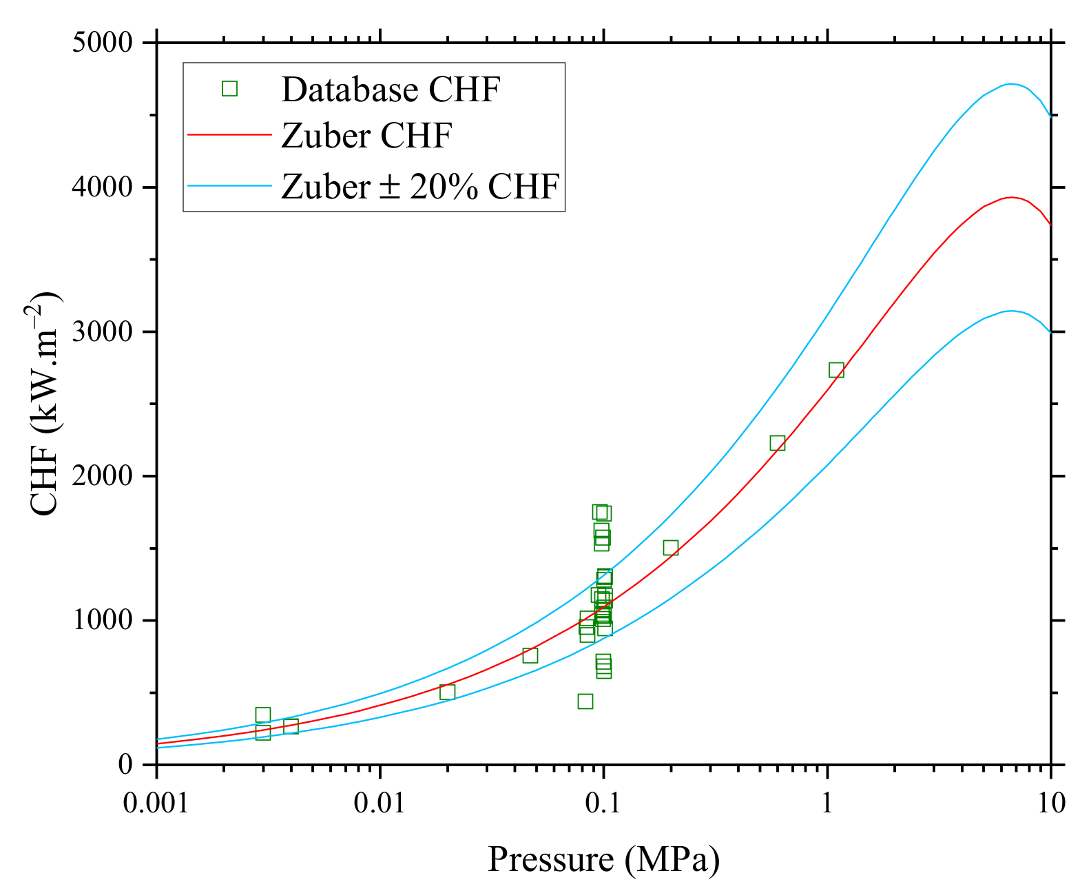
In order to check the quality of the collected data, the CHF experimental data for deionized water at different pressures are presented. The DI water pool boiling experiment is usually performed prior to NF pool boiling experiments to validate the experimental apparatus, as well as to obtain a standard value for comparison. Figure 5 presents the DI water pool boiling CHF values collected from the literature [1,2,4,13,15,17,18,19,20,21,22,23,24,25,26,27,29,31,32,33,35,36,37,38,39,40,41,42,43] for saturated temperature as a function of pressure. Zuber’s prediction [54] was also plotted for comparison.

Zuber’s correlation was developed in 1959 and it considers only fluid properties in CHF prediction. Zuber observed that CHF is the limit when a vapor layer develops around the surface, creating a very unstable region given by the difference between the vapor and fluid densities, known as Rayleigh–Taylor instability. Zuber’s correlation is given by Equation (2):

$$q_{cr}^{″}=\frac{\pi }{24}{\rho }_g{h}_{fg}{\left[\frac{\sigma \left({\rho }_f-{\rho }_g\right)g}{{\rho }_g^2}\right]}^{0.25}$$

(2)

where ${\rho }_g$ is the gas density, $h_{fg}$ is the enthalpy difference between the gas and liquid, ${\rho }_f$ is the liquid density, $g$ is the gravity constant, and $\sigma$ is the surface tension between the liquid and gas.

It can be observed that most of the datapoints were in very good agreement with Zuber’s correlation. However, a small number of datapoints fell outside of the $\pm$20% range for pressure equal to atmospheric pressure.

Most of the experiments were conducted under atmospheric pressure conditions, which explains the datapoint concentration of around 0.101325 MPa. However, determining the experimental atmospheric pressure and saturation temperature was not a straightforward task since most of the studies do not make these conditions clear. Ciloglu [21], for example, only mentions atmospheric conditions, but considering the research facility location, those conditions were far away from sea level, which caused significantly different CHF values. The effects of experiments performed in different sea level conditions were taken into account here.

As can be observed in Figure 5, CHF versus pressure follows a growing trend until reaching its peak at around 6 MPa; then, it turns back to a decreasing trend. That is explained by the competition between the fluid properties considered in Zuber’s correlation, as seen in Equation (1), at different pressures, i.e., liquid and gas densities, enthalpies, and surface tension. In low-pressure ranges, vapor density increases considerably with increasing pressure, impacting CHF the most, while in high-pressure ranges, the surface tension and the vaporization latent heat are the most affected, both decreasing with the pressure increase.

4.2. Full Nanoparticle Database Analysis

An analysis was carried out considering the full NP database. ML hyperparameter optimization and the model’s training require many datapoints for better performance; hence, 80% of the initial database was used to perform these tasks. After database preprocessing, split, and hyperparameter optimization, the ML model was implemented using the training dataset, and cross-validation was applied using the remaining 20% of the datapoints to evaluate the model’s generalization. The ML model implementation was repeated ten times, using ten different splits in the original database to show that the model solved the problem for different input datasets. Lastly, three ML models were built, and their predictions were compared to the collected experimental data trends, as discussed in Section 5.

4.2.1. SVR Analysis for the Full NP Database

As previously discussed, four SVR hyperparameters were optimized using the full NP database: the kernel function, C value, gamma coefficient, and $\epsilon$ (margin). The kernel function has only four possible values: linear, polynomial, sigmoid, or radial basis function (RBF). The C value range was selected from 0.01 to 1, with increments of 0.01, and from 1 to 1000, with increments of 10, leading to a total of 10,000 possibilities. The $\epsilon$ range was selected from 0.01 to 1, giving a total of 100 possibilities. The gamma coefficient range was selected from 0.05 to 1, with increments of 0.05, and from 5 to 100, with increments of 5, leading to a total of 40 possibilities. As the selected hyperparameter search space was relatively small, it was optimized using the Sklearn grid search tool. This tool tries all the possible combinations, which are given as a list of arguments, and displays the combination that obtains the best score. The grid search was performed individually for each kernel function. Each kernel function had a different search space. The linear kernel function only used C and $\epsilon$ values in the model. Consequently, its search space had 1,000,000 possibilities. The polynomial function is the only one that has an extra hyperparameter, the degree of the polynomial function. This kernel function considered C, $\epsilon$, and gamma values, giving a total search space of 40,000,000 for each degree. The sigmoid and RBF kernel functions both had the same search space of 40,000,000 each and considered the C, $\epsilon ,$ and gamma values. The best obtained score for each kernel function run is presented in

Table 2. SVR hyperparameter optimization.

Kernel Function	Degree	C Value	Epsilon	Gamma Coefficient	Training Score
linear	-	0.46	0.1	-	0.2178
poly	3	396	0.197	100	0.3639
RBF	-	141	0.05	10	0.7425
sigmoid	-	11	0.17	0.1	0.2250

.

The scores provided by the SVR model are the R² coefficient of determination, as seen in Equation (3):

$$R^2=1-\frac{SSR}{SST}=1-\frac{\sum {\left(y_i-{\widehat{y}}_i\right)}^2}{\sum {\left(y_i-\overline{y}\right)}^2}$$

(3)

Equation (3) represents how well a regression model is fitted to the data and gives a value between 0 and 1. SSR is the sum of the squared residuals, given by the sum of the difference between each real value ($y_i$) and each related model’s predicted value (${\widehat{y}}_i$) squared, while SST is the sum of the squared total, given by the sum of the difference between each real value ($y_i$) and the mean of the predicted values ($\overline{y}$) squared. The higher the value, the better the model is fitted to the data.

These results show that the RBF kernel is the one that provides the best fitting; this can be explained by the nature of the RBF. The RBF applies an exponential kernel to the data, which means using an infinite-dimensional function to transform n-order data into higher-order data. After this relation between the transformed data is chosen, an $\epsilon$-tube can be fitted to the data.

The RBF hyperparameter values, as given in Table 2, were selected and used to fit an SVR model to the data. The results for ten different runs, which represent different training and validation datasets, are presented in

Table 3. SVR model full NP database implementation.

Run	Training Score	Testing Score
1	0.8936	0.7631
2	0.8890	0.7250
3	0.8991	0.7996
4	0.8946	0.6921
5	0.8788	0.8402
6	0.8940	0.6539
7	0.9086	0.7166
8	0.9074	0.7359
9	0.9039	0.6912
10	0.8922	0.8157

.

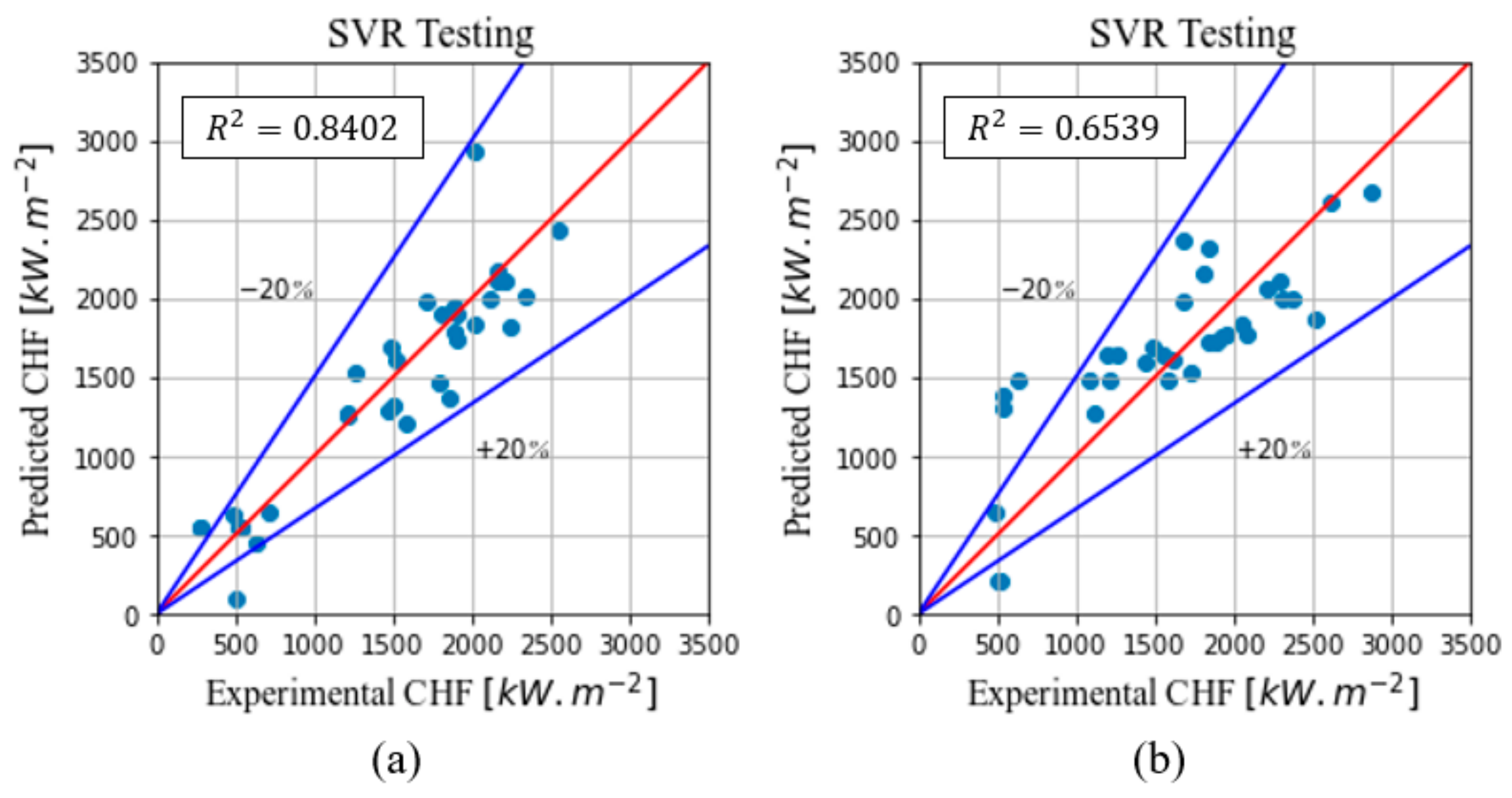
Based on Table 3, different scores were obtained for different inputs, as given by different splits in the initial database. The training score had low variation, while a small number of runs, such as runs #4, #6, and #9, presented testing scores lower than 70%. Figure 6 presents the best and worst CHF testing data cross-validations, runs #5 and #6, respectively.

A reduction in the score between the training and testing data fittings was expected. However, consistent scores were also expected for both the training and testing fittings. Hence, the results obtained in Table 3 bring three possible implications: (1) the database could be too small to be used in the SVR model or it could have some outliers not captured in the initial data evaluation; (2) the SVR model cannot correctly solve the problem; and/or (3) the model’s fitting is overfitting the training data. The ML models implemented in the following sections will help to determine which one of these three interpretations is correct. The predicted CHF values obtained from run #5 will be compared to the experimental CHF values and the other models in Section 5.

4.2.2. MLP Analysis for the Full NP Database

As mentioned in Section 3, four MLP hyperparameters were optimized by randomized search using the full NP database: (1) number of hidden layers; (2) number of neurons in each hidden layer; (3) neuron activation function in each hidden layer; and (4) the model optimizer. The MLP search space can be incredibly large depending on its considerations. For example, considering 2 to 10 hidden layers, 2 to 10 neurons per layer, 5 activation function possibilities for each layer, and 5 possible model optimizers, the total search space size is around 1.7 × 10¹⁷. Thus, it is important to properly select those ranges to reduce the search space to a more testable size. In this work, the decision was to use 2 to 5 hidden layers; 20 to 50 neurons per layer, with increments of 5 neurons; 3 activation functions for each layer; and 3 possible model optimizers; this gave a search space size of around 12,000,000 possibilities.

The three activation functions selected were sigmoid, hyperbolic tangent “tanh”, and rectified linear unit “relu”, which are three of the most used activation functions for the ANN models. Sigmoid outputs a value between 0 and 1, while hyperbolic tangent outputs a value between $-$1 and $+$1. The “relu” function provides a non-linear transformation of the input with an output with the same value as the input, if it is positive, or 0, if it is negative.

In addition, the three model optimizers considered were RMSprop, Adam, and Nadam. These three models are adaptive, meaning that they modify the learning rate after each epoch. RMSprop stands for root mean square propagation, a method that adapts the learning rate by dividing it by the square root of the moving average (first momentum) of the squared gradient. This method takes longer steps into the weight updates and smaller steps into the bias updates, which speeds up the model’s convergence. Adam comes from “adaptive moment estimation” and it combines adaptive gradient and RMS propagation by adding the second momentum (the uncentered variances) to the weight update. In other words, it calculates an exponential moving average of the gradient and the squared gradient [55]. Finally, Nadam combines Adam and NAG (Nesterov accelerated gradient) which updates the momentum term before computing the gradient [56].

For the MLP hyperparameter optimization, three independent runs were performed, one for each optimizer option. Each run built 3000 different ANNs, which ran for 200 epochs. The MLP scores are presented in

Table 4. MLP hyperparameter optimization.

Run	Number of Hidden Layers	MLP Structure	MLP Activation Functions	Model’s Solver	Training Score
1	4	4-50-50-40-40-1	relu-relu-tanh-relu-tanh	RMSprop	0.8422
2	3	4-50-50-50-1	relu-relu-relu-sigmoid	Nadam	0.8459
3	5	4-50-50-30-35-40-1	relu-relu-relu-relu-tanh-sigmoid	Adam	0.8511

; these are, as shown in the SVR model, given by the coefficient of determination R² related to the training data.

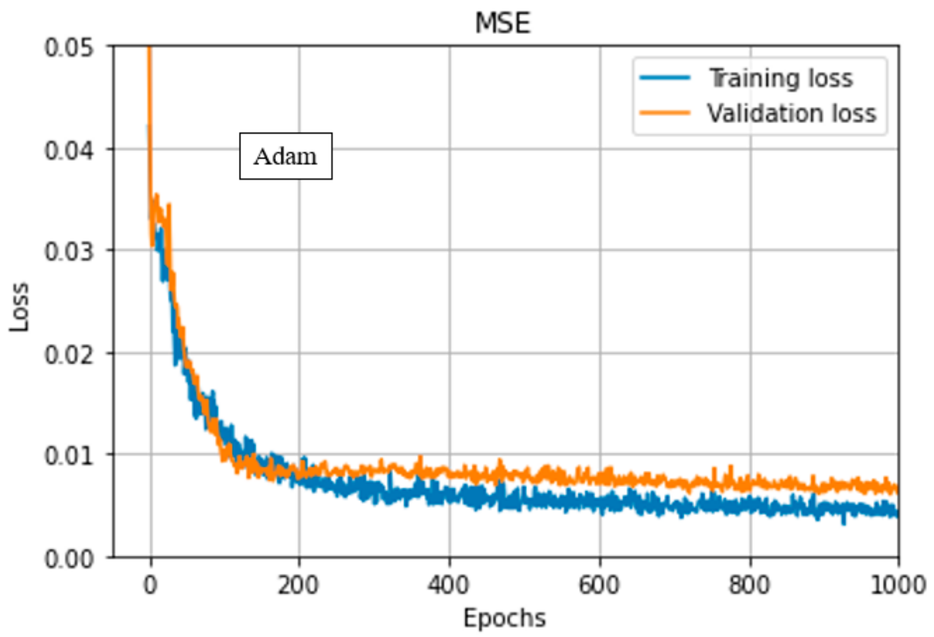
Those initial results showed that the Adam optimizer presented the best score after 200 epochs compared to Nadam and RMSprop. However, the difference between the three scores was minimum; hence, these three MLPs were trained for 1000 epochs for further comparison. Figure 7 shows the training loss function obtained for the Adam optimizer.

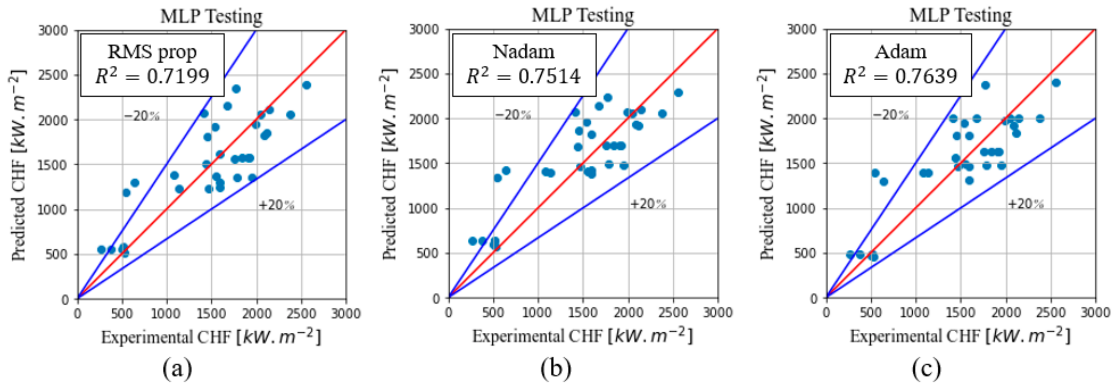
The three MLP models built presented similar curves to the one presented in Figure 7. This curve shows that the model had a good fit for the data. Overfitting to the training data would be characterized by the training and validation loss curves’ distance starting to increase at some point in the plot, which never happens. A gap between the training and validation loss is expected. Figure 8 shows a CHF testing data cross-validation comparison between the three MLP solvers.

It can be observed that the structure built with the Adam solver presented the best testing score. Therefore, the Adam solver with its related structure, run #3 in Table 4, was used as the MLP model to be compared to the other two ML models. Ten runs with different splits, which represent different training and validation datasets, were carried out for 1000 epochs, and the results are presented in

Table 5. MLP model full NP database implementation.

Run	Training Score	Testing Score
1	0.9008	0.7605
2	0.8778	0.8755
3	0.8952	0.8702
4	0.9076	0.8502
5	0.8859	0.8177
6	0.8994	0.8142
7	0.8884	0.8278
8	0.9073	0.8132
9	0.9048	0.8034
10	0.8948	0.8283

.

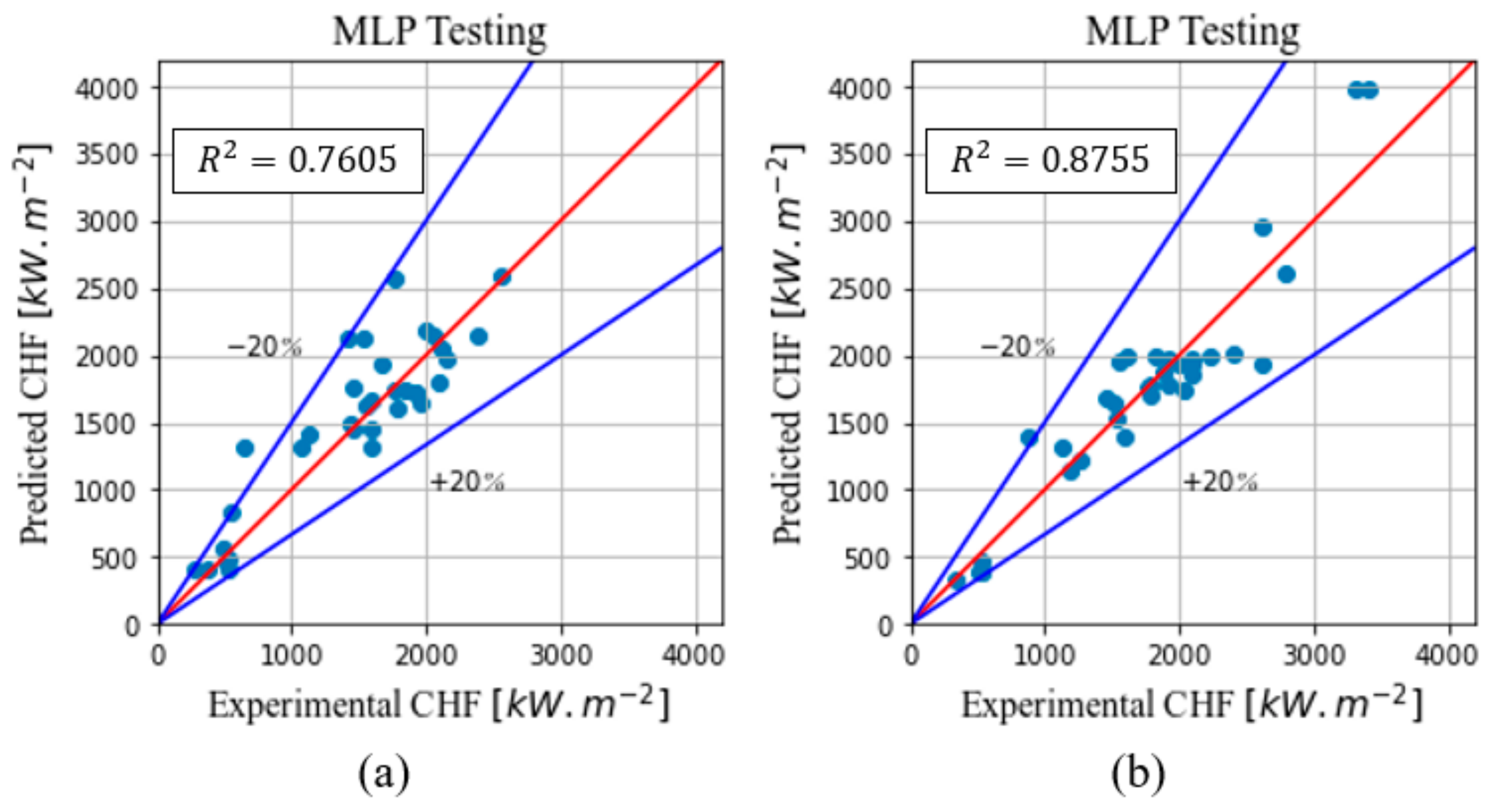
The results show that the built MLP had a low variation in the training score and that only run #1 presented a testing score lower than 80%. Figure 9 presents the worst and the best CHF testing data cross-validations, runs #1 and #2, respectively.

The MLP model results, as given in Table 5, show that this model gave better predictions than the SVR model; hence, it was more suitable to solve the problem. In addition, the previously opened discussion about the SVR model and the dataset is now closed. Based on the MLP performance, it seems there were no outliers in the dataset. Finally, it cannot be known whether the SVR model overfitted the training dataset or not. That could only be known by applying other overfitting checking techniques. On the other hand, it can be known that the MLP model did not achieve any overfitting, as can be seen in the behavior of the loss curves in Figure 7. The RF model will be presented in the next section.

4.2.3. RF Analysis for the Full NP Database

Three hyperparameters were optimized using a randomized search for the RF model: the number of trees, the maximum features, and the maximum samples. The number of trees is an important hyperparameter of any RF model, and it was evaluated in the range of 1 to 500. The maximum feature options evaluated were: “sqrt” and “log2”. The square root of the number of features is selected when “sqrt” is used, while “log2” sets the base 2 logarithm of the number of features. The maximum samples were evaluated for five different possibilities: 0.2, 0.4, 0.6, 0.8, and 1.0. It summed up a search space of 5000 possible combinations. The hyperparameters were optimized by applying the Sklearn random search tool. Ten different runs were carried out, with 250 iterations each, in the search space for the same input data. The results are presented in

Table 6. RF hyperparameter optimization.

Run	Number of Iterations	Number of Trees	Maximum Features	Maximum Samples	Training Score
1	250	15	sqrt	1.0	0.7636
2	250	53	sqrt	1.0	0.7729
3	250	15	sqrt	1.0	0.7553
4	250	72	sqrt	1.0	0.7541
5	250	34	log2	1.0	0.7648
6	250	34	log2	1.0	0.7595
7	250	82	sqrt	1.0	0.7582
8	250	61	log2	1.0	0.7580
9	250	61	log2	1.0	0.7618
10	250	15	sqrt	1.0	0.7585

. Notice that there were ten independent runs with 250 iterations each but that does not mean that 2500 different possibilities were tested, i.e., there is a possibility of the same set of hyperparameters being selected in more than one of those independent runs. However, many possibilities were indeed covered.

A second hyperparameter optimization was carried out for a narrowed search space based on the first optimization results. The scores given by the RF model also corresponded to the coefficient of determination R². This time, the range used for the number of trees was limited to the range 1–150, because smaller trees were preferred. Both maximum feature options were selected. Finally, the maximum sample options selected were 0.7, 0.8, 0.9, and 1.0, reducing the search space to 1200 possible combinations. All combinations were tested by the grid search tool implementation. For this last optimization, the best score was obtained for the model with 49 trees, “sqrt” maximum features, and 1.0 maximum sample. Those hyperparameters were then applied to build a model for ten different input datasets, as shown in

Table 7. RF model full NP database implementation.

Run	Training Score	Testing Score
1	0.9636	0.9035
2	0.9596	0.7730
3	0.9548	0.5145
4	0.9735	0.7346
5	0.9703	0.8601
6	0.9624	0.8022
7	0.9658	0.7267
8	0.9640	0.8173
9	0.9639	0.8179
10	0.9697	0.7479

.

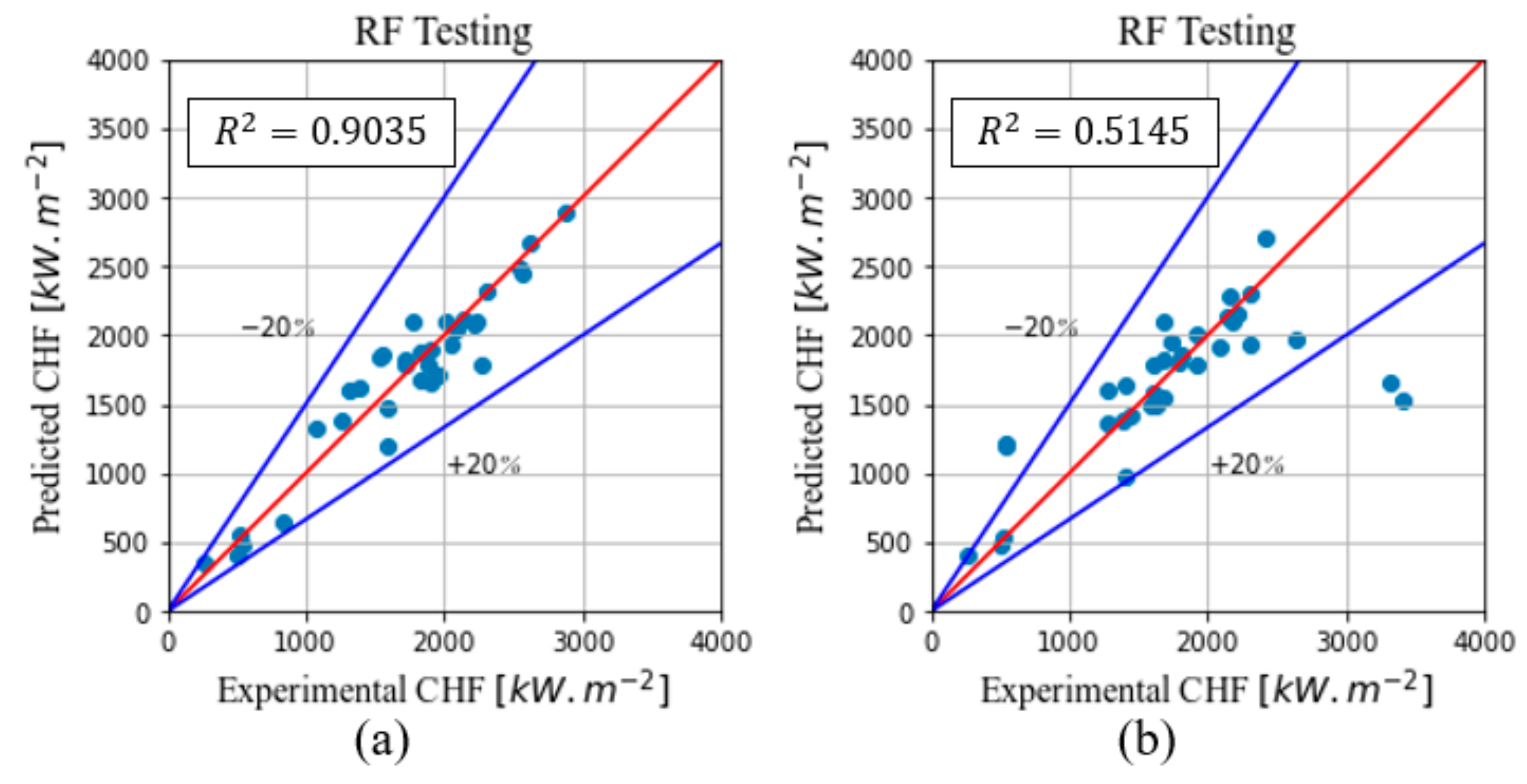
As can be seen in Table 7, the training scores were higher than the ones obtained for the two previous ML models. However, the testing scores presented higher variability compared to the other two ML models, which was not desirable. The best and the worst obtained scores, runs #1 and #3, respectively, are shown in Figure 10.

While the predicted and real values had good agreement for run #1 in Figure 10a, a similarly good agreement was not observed for run #3 in Figure 10b. Three datapoints were far away from the $\pm$20% range. To determine which built ML model was the best one to solve the NF pool boiling CHF, the performances of the three ML models are compared in the next section.

4.3. Machine Learning Models’ Performance

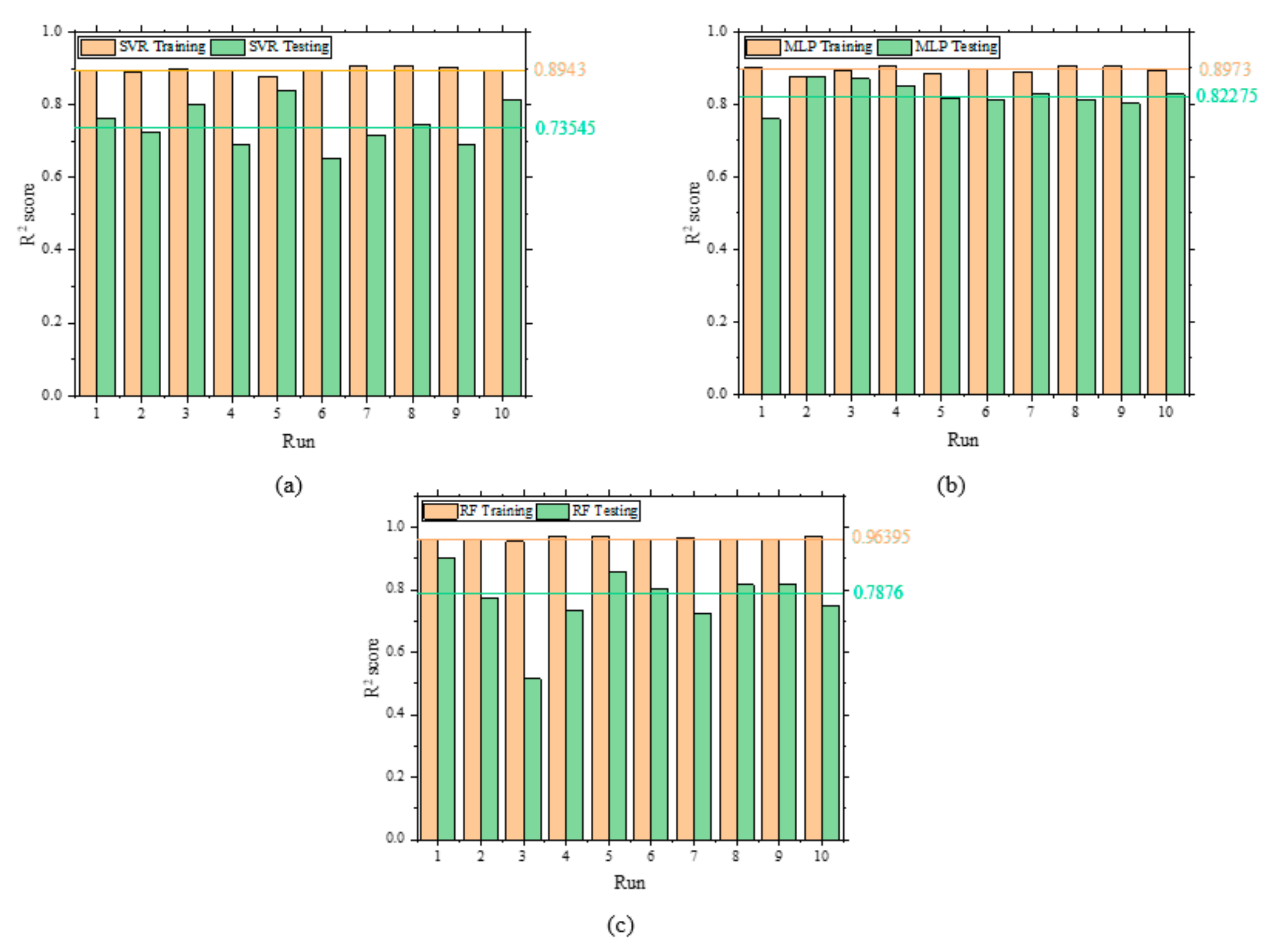
For a better understanding of the three ML models’ performance, the 10-run results in Table 3, Table 5, and Table 7 were plotted in a column graphic, as shown in Figure 11.

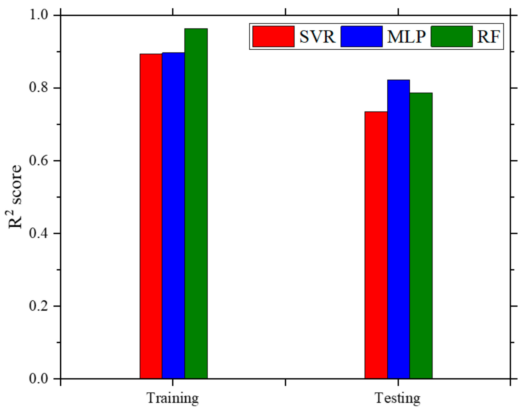
It can be observed that the training R² scores are high and present a relatively low variability for all the three ML models. However, when the testing R² score was analyzed, the MLP model presented not only the highest mean value of 0.82275, but also the lowest variability among the three models. To emphasize the MLP model’s better performance, the mean R² score values are plotted in Figure 12.

Therefore, after building these three models and comparing their performances, the MLP was chosen as the best model since it presented low variability and good predictions. The SVR had limited prediction improvement and the RF had high variability. Hence, the built MLP model of run #2 in Table 5 was used to obtain the predictions used in the next section. The comparisons between the ML model predictions and the experimental data, as well as the importance of the selected features, are also discussed next.

5. Discussion on Parametric Effects

In order to evaluate the importance of the selected features in relation to CHF, three feature importance models were compared based on the database: (1) the mean decrease impurity (MDI); (2) the permutation model; and (3) the drop column model. Before running these models, a column of random numbers (as a sixth feature), generated using the random.randn function in the NumPy library, was inserted in the dataset. As random numbers have, in theory, zero importance to any model, if any feature presents an importance smaller than the one obtained for the random number, this feature is considered not important to the model.

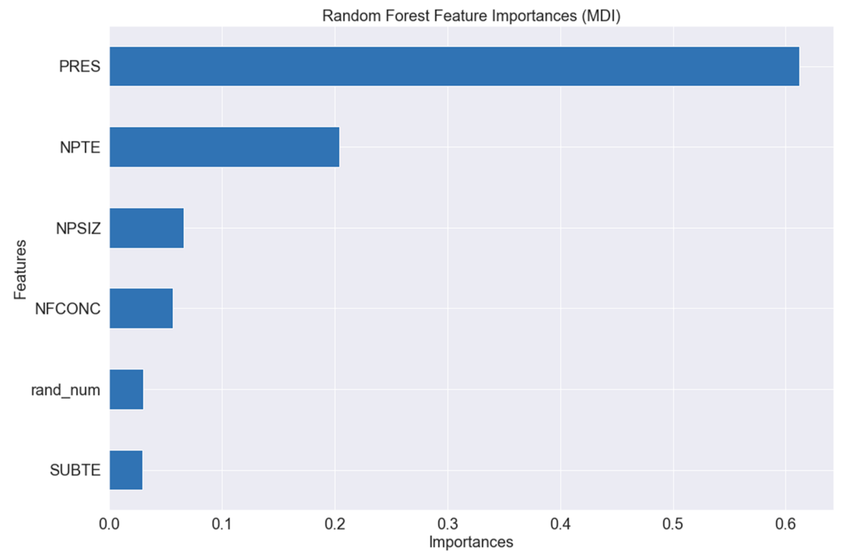
Of the three ML models applied to the database, the RF regressor is the only one that provides a feature importance analysis. This analysis is also known as MDI and it implements the Gini importance, which measures how much a feature reduces the model’s loss function when creating the trees. A bar plot was generated based on the results obtained for the training dataset, as shown in Figure 13.

In Figure 13, Figure 14, Figure 15 and Figure 16, PRES is the pressure, NPTE is the NP thermal effusivity, NP is the NP size, NPCONC is the NP concentration, rand_num is the random number, and SUBTE is the substrate thermal effusivity.

As shown in Figure 13, the importance bar for substrate thermal effusivity (SUBTE) is smaller than the random number one, meaning that this feature was not important for the model. This first importance evaluation was compared to the other two models. The MDI model is known for its limitation in relation to high cardinality features. In general, they are more biased toward high cardinality features than to low ones.

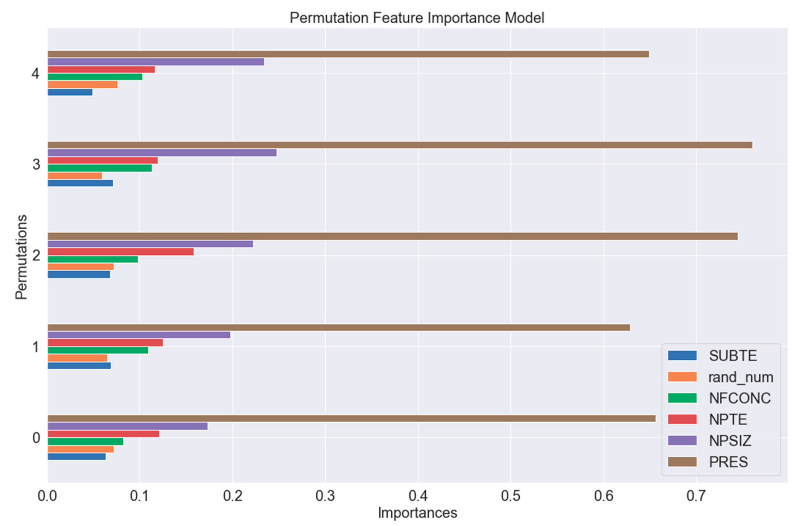
The second feature importance model applied was the permutation model. It evaluates the features’ importance by changing one feature datapoint at a time and evaluating how this change affects the model accuracy, as can be seen in Figure 14.

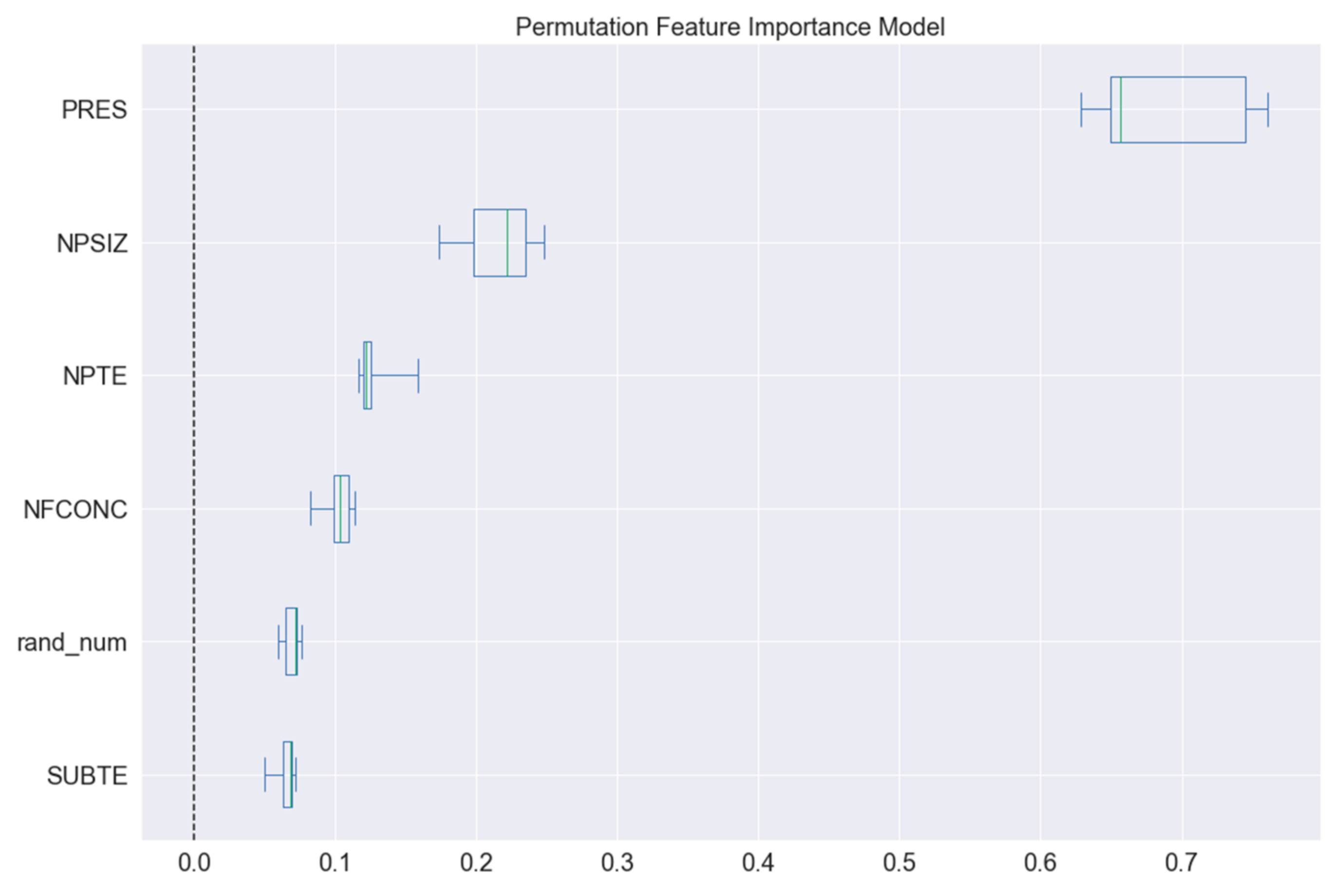
As shown in Figure 14, in all the permutations pressure was the most important feature, as one might expect, followed by NP size, while substrate thermal effusivity was the only feature that exhibited smaller importance than that of a random number. The results obtained by this importance evaluation are slightly different from the one provided by the RF regressor (MDI). However, both models agree that pressure is the most important feature, NP size is the second most important, and substrate thermal effusivity is not important to the model. The most common plot form used to present a permutation feature importance is the merging of all the permutations, as shown in Figure 15.

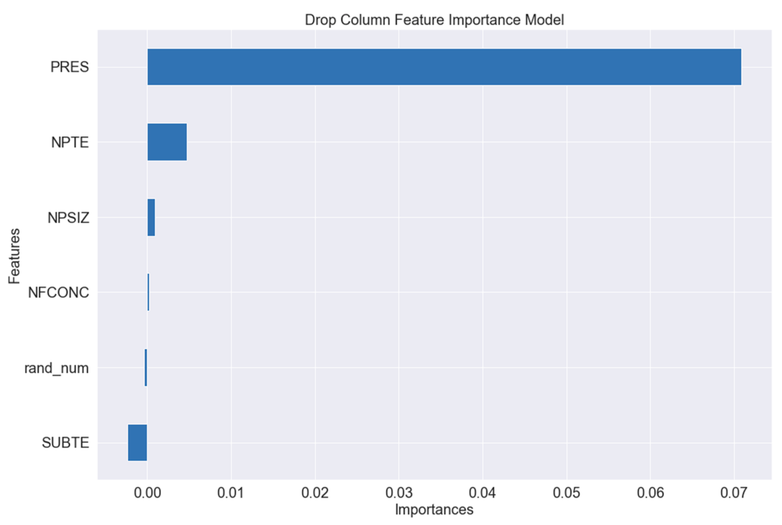
Finally, the third feature importance evaluation method, known as the drop column model, which drops each feature column at a time and evaluates how the model’s performance is affected, is presented in Figure 16.

According to Figure 16 and all the other implemented feature importance models, pressure was the most important feature in NF pool boiling CHF. Moreover, the three models show agreement regarding the fact that substrate thermal effusivity does not have a relevant impact on NF pool boiling CHF. The behavior of each feature in NF pool boiling CHF is investigated next.

5.1. CHF × Pressure

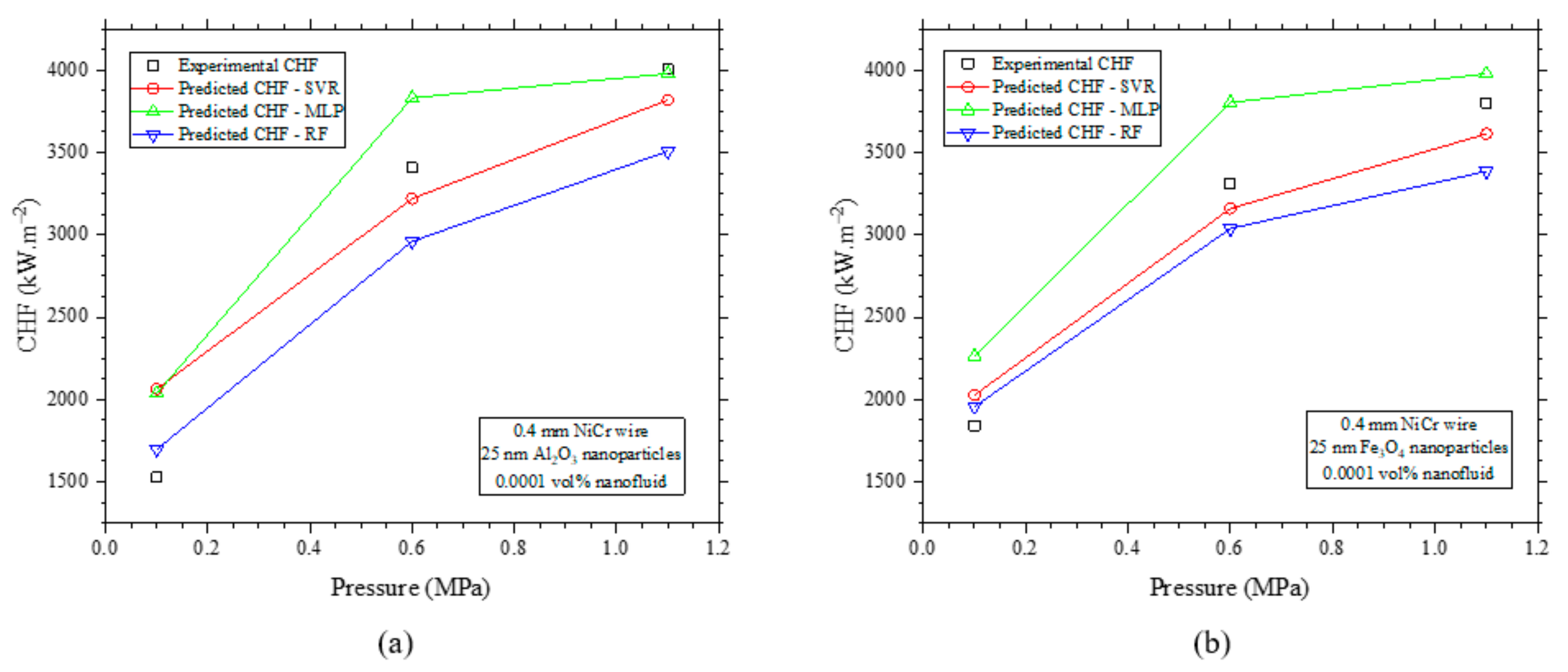
According to all three of the feature importance models previously discussed, pressure is the feature that affects NF pool boiling CHF the most. Figure 17 presents the experimental and the predicted CHF values for the different pressures, while the other features are kept fixed.

As presented in Figure 5, water pool boiling CHF increases as the pressure increases. Following the same behavior, NF pool boiling CHF also increases as the pressure increases. However, the CHF ratio between NF and DI water decreases as the system pressure increases; in other words, less accentuated NF CHF improvements are obtained at higher pressures, as was also observed in refs. [17,19]. According to previous studies, three main bubble dynamics are important to explain CHF modification with increasing pressure: (1) bubble size decrease due to a decrease in the density ratio between liquid and vapor; (2) the average bubble frequency increase; and (3) the nucleation site density increase. NF affects CHF dynamics in the following ways:

-

The decrease in bubble size with the system pressure increase is well known. The bubble size is determined by the force balance between the bubble internal and external pressures. Accordingly, the bubble at higher system pressures requires higher internal pressure forces to nucleate. NP deposition increases the wettability (lowering contact angle) of the surface, which requires larger bubble nucleation diameters [57] for a fixed pressure.

-

The average bubble frequency in nanofluid pool boiling is significantly higher compared to water pool boiling [19]. This is attributed to the enhanced wettability resulting from nanoparticle deposition, which improves the surface rewetting process immediately after bubble departure.

-

At higher pressures, higher heat fluxes are needed to achieve CHF and, therefore, more cavities are activated on the surface, increasing the nucleation site density. The number of active sites on the surface is also increased by the NP deposition process, delaying CHF at higher heat fluxes.

According to Figure 17, all three ML models were capable of giving good predictions based on pressure and NF characteristics.

5.2. CHF × NP Size

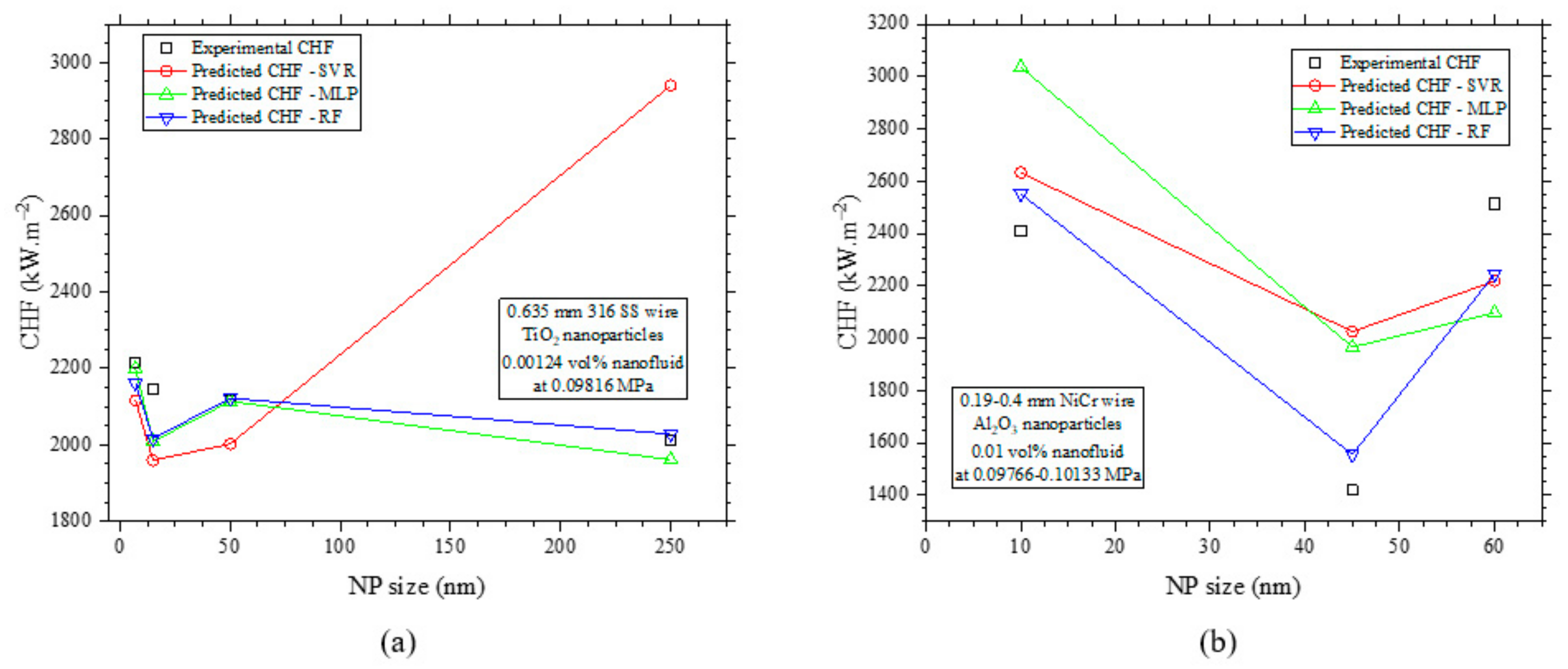
According to all three feature importance models previously discussed, NP size is the second contributor to NF pool boiling CHF enhancement. Figure 18 presents the experimental and the predicted CHF values for different NP sizes, while the other features are kept constant.

According to Figure 18a, the increasing TiO₂ NP size decreases CHF. Stange et al. [5] investigated how CHF changed for TiO₂ NP pool boiling using different NP sizes. They believe that this can be explained by the NP attachment to the surface. Larger NPs tend to form a non-stable layer that can easily detach during the boiling process, forming a non-uniform coating on the surface. On the other hand, performing an electrophoretic deposition (EPD) technique on a few samples, they observed a much more uniform NP layer attached to the surface, which provided better CHF values.

Ciloglu provides an extra discussion in his study [21] on the effect of NP size. He brings to the discussion an important parameter, the surface particle interaction parameter ($\psi$), which is a ratio of the average surface roughness and the average particle diameter. Based on this parameter, the boiling performance improves when $\psi \gg 1$; it remains the same if $\psi ~ 1$; or it can even deteriorate when $\psi \ll 1$. Therefore, this indicates that CHF is probably affected by the pairing of the substrate and the NP (roughness and NP size), which can lead to the behavior observed in Figure 18b.

Moreover, the SVR model prediction loses its track in Figure 18a; hence, both the RF and the MLP models can give good CHF predictions based on NP size.

5.3. CHF × NF Concentration

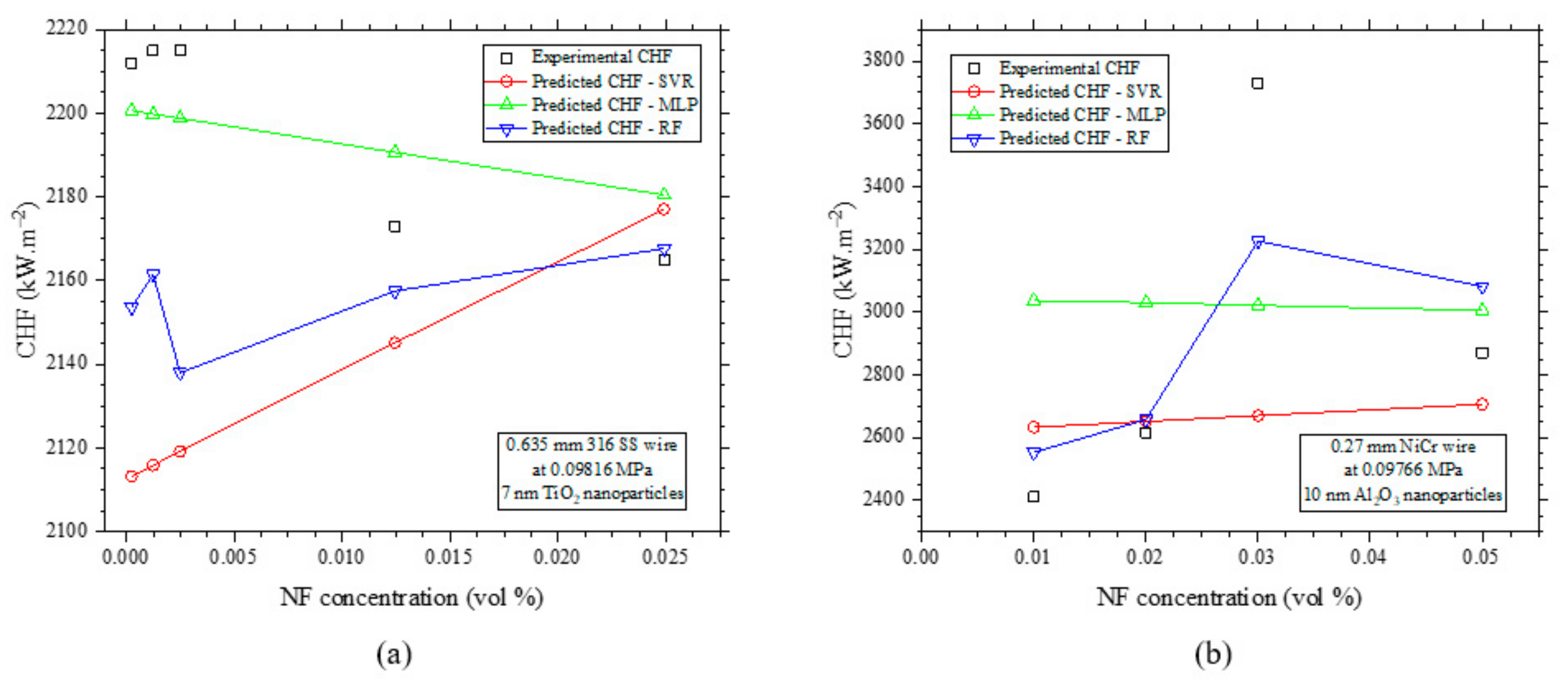
According to all three feature importance models previously discussed, NF concentration also plays a small role in NF pool boiling CHF. Figure 19 presents the experimental and the predicted CHF values for different NF concentrations, while the other features are kept fixed. At higher NP concentrations, the CHF deteriorates, as shown in Figure 19b. The impact of NF concentration is discussed by several authors and will be discussed next to achieve a more generalized understanding of the phenomenon.

In Figure 19, both NP concentration ranges are very low. Ciloglu [21] observed a CHF improvement in a water-based SiO₂ NF pool boiling experiment in the 0.01–0.1 vol.% range, using a copper semi-sphere as a heating element. He attributed the CHF improvement to the surface roughness improvement after NP deposition. The average surface roughness of bare wire, before conducting the pool boiling experiment, was 3.27 nm, and it changed to 16.58 nm for the highest concentration. However, higher roughness does not necessarily mean higher CHF.

Kumar et al. [13] observed a maximum CHF improvement at a certain NF concentration and then a drop in CHF improvement in two water-based pool boiling experiments using a nichrome wire as a heating element: (1) Al₂O₃ NF pool boiling using six different concentrations, ranging from 0.01 to 0.1 vol.%, and (2) Fe₂O₃ NF pool boiling using five different concentrations, ranging from 0.01 to 0.09 vol.%. They attributed the CHF improvement in NF to the enhancement of the surface wettability, which was due to NP deposition on the heating surface and to the modification of the base fluid thermal conductivity, which increases the heat dissipation between the surface and the fluid. At high concentrations, the NP in the NF starts an aggregation process, which leads to settling of the NP aggregation and, hence, a change in the fluid’s thermal properties and its stability. Taking a different approach, Kim et al. [3] do not believe the hydrodynamic instability theory explains NF CHF improvement since NF thermal properties are very similar to the base fluid properties.

According to Figure 19a, due to these competitive effects all three ML models showed limited CHF prediction capabilities according to the NF concentration, with MLP showing the best prediction values. According to Figure 19b, the analysis changed slightly. Once again, the three models presented limited CHF prediction capabilities with NF concentration; this time the RF was the one presenting the best prediction values.

5.4. CHF × Substrate Thermal Effusivity

According to all three feature importance models previously discussed, the effect of substrate thermal effusivity was considered negligible to NF pool boiling CHF. However, Stange et al. [5] reported that titanium (Ti) NPs have better adhesion to zirconium than other oxide NPs. This brings up another discussion about NF pool boiling: the selection of the pairing of the heating element and the nanoparticle type can also be very important in achieving further CHF improvements. Yao et al. [17] discuss different NP types, which, due to their different properties, become attached to the surface of the heating element in different forms, producing different microstructure modifications. A rougher layer was generated in Al₂O₃ NF boiling compared to SiO₂ NF boiling, which means that this layer was more porous; hence, it was more susceptible to bubble generation. This suggests that the pairing of the heating element and the NP type should be considered as a feature for future work due to the different bonding levels and affinities between different pairs of materials; therefore, a decision was made to keep the substrate effect on the model. However, it is emphasized that additional research needs to be performed in this area to show its importance. Among all the datapoints in the developed database, a pool boiling experiment at 1.1 MPa combining NiCr wire with a 0.0001 volume percent concentration of 25 nm Al₂O₃ NP presented the highest CHF value of 4006 kW/m².

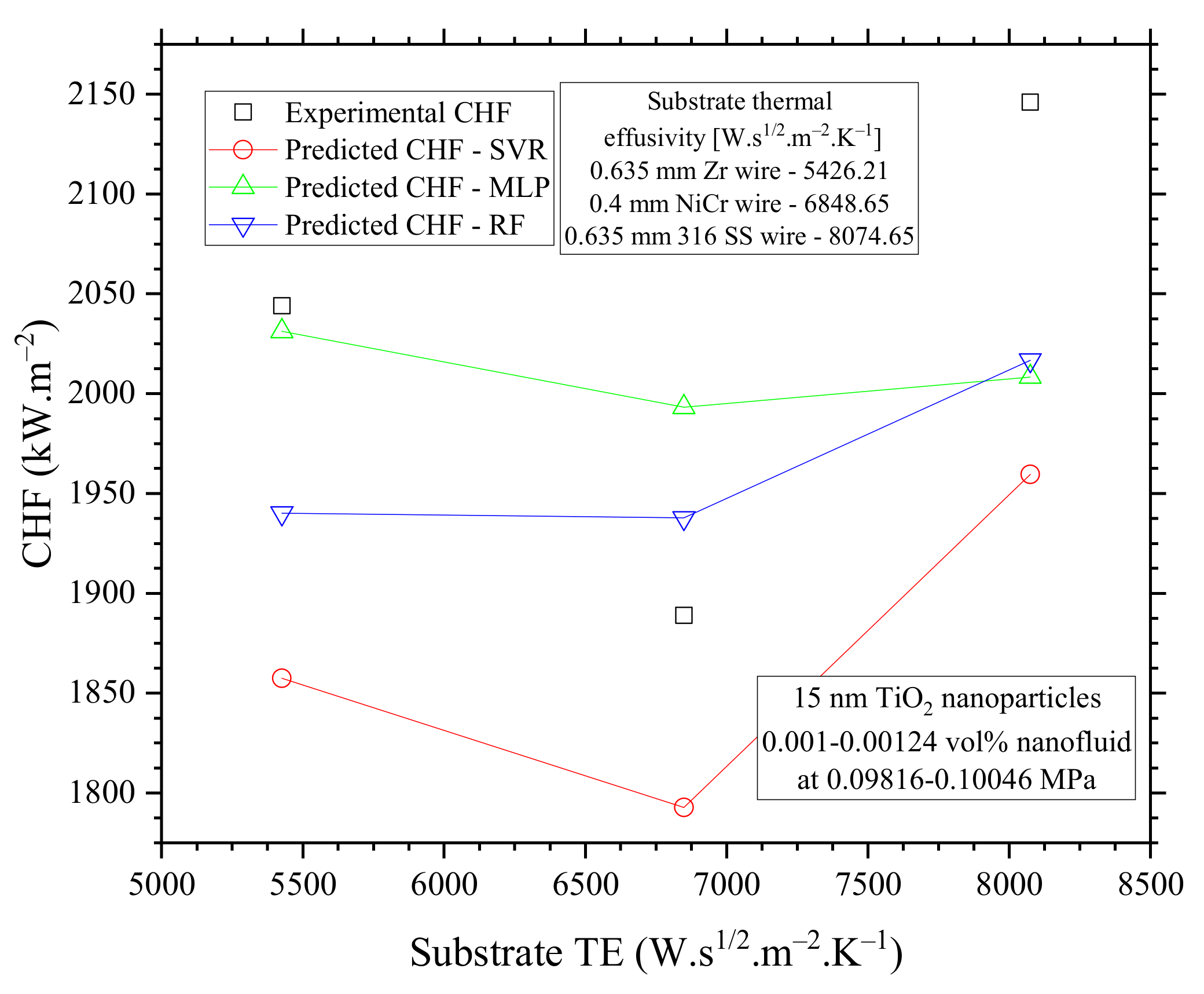
The CHF trend for the three different substrates (Zirconium, Nichrome, 316 stainless steel) is shown in Figure 20 as a function of substrate thermal effusivity.

According to Figure 20, all three models were able to capture the trend of CHF based on substrate thermal effusivity, even though it had a small effect on CHF, as concluded from the feature importance of previous analyses. Again, RF and MLP were the ones providing the best CHF prediction values.

5.5. Secondary Effects

The effects of roughness, wettability, and wickability on CHF modification after NF pool boiling experiments were discussed in previous studies [15,21,24,29]. They reported that these three features have a close relationship with each other, which also depends on the NP type, size, and NF concentration. The NP attaches to the surface microstructure during the boiling process creating a porous layer on the surface. This layer can affect CHF in two different ways: (1) it can modify the number of nucleation sites on the surface, changing the surface wettability, which changes CHF, and (2) if a thick layer is created, the thermal resistance increases, which decreases CHF. Hence, the NP type, size, and NF concentration would modify the surface characteristics differently, affecting the total NP deposition and the thickness of the layer. Therefore, the nanoparticle-coated surface layer (roughness) effect is balanced between those two former mechanisms, i.e., higher roughness does not necessarily mean higher CHF, as previously discussed.

In addition, NP deposition changes wickability, also known as capillary wicking or the capillary effect, which impacts the surface rewetting speed [4]. The formation of a porous layer increases the adhesion and surface tension forces which spread the fluid on the surface (decreasing the contact angle between the fluid and the surface). That motion postpones CHF since surface rewetting happens much faster than on a non-coated surface.

Other secondary effects have been investigated, such as heating element boiling time [9,18,29], boiling at different heat fluxes [18,29], and boiling in different shapes, such as wires, ribbons, flat surfaces, etc. [27,30]. Those characteristics also have secondary effects on NF pool boiling CHF.

5.6. Final CHF Model

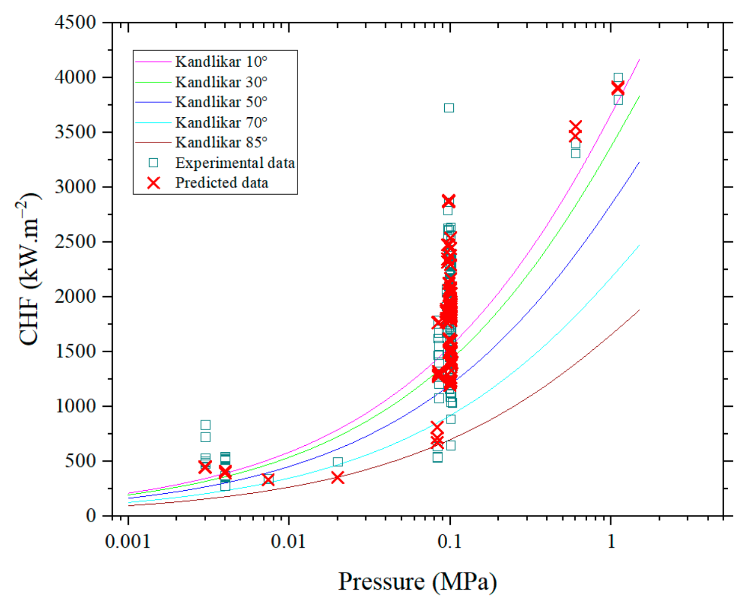
Based on the analyses previously discussed in this section, it can be concluded that the systematic development of the ML models successfully demonstrated the quantitative contributions of each parameter on the CHF enhancement, with SVR presenting the less accurate CHF predictions, while RF and MLP presented the most accurate CHF predictions. As the MLP model also showed lower variability compared to the RF one, the built MLP model was applied to generate CHF predictions, which were compared to the database values and to Kandlikar’s model [50], assuming no heating element angular orientation (heating element always facing upwards) and a large variability of contact angles: 10$°$, 30$°$, 50$°$, 70$°$, and 85$°$, as shown in Figure 21.

Figure 21 shows that the MLP predictions are more accurate than Kandlikar’s predictions. Furthermore, Kandlikar’s model requires the receding contact angle, which, in most cases, is not measured in the studies. Thus, MLP provides much simpler and more straightforward predictions based on training using a database and the NF’s main characteristics.

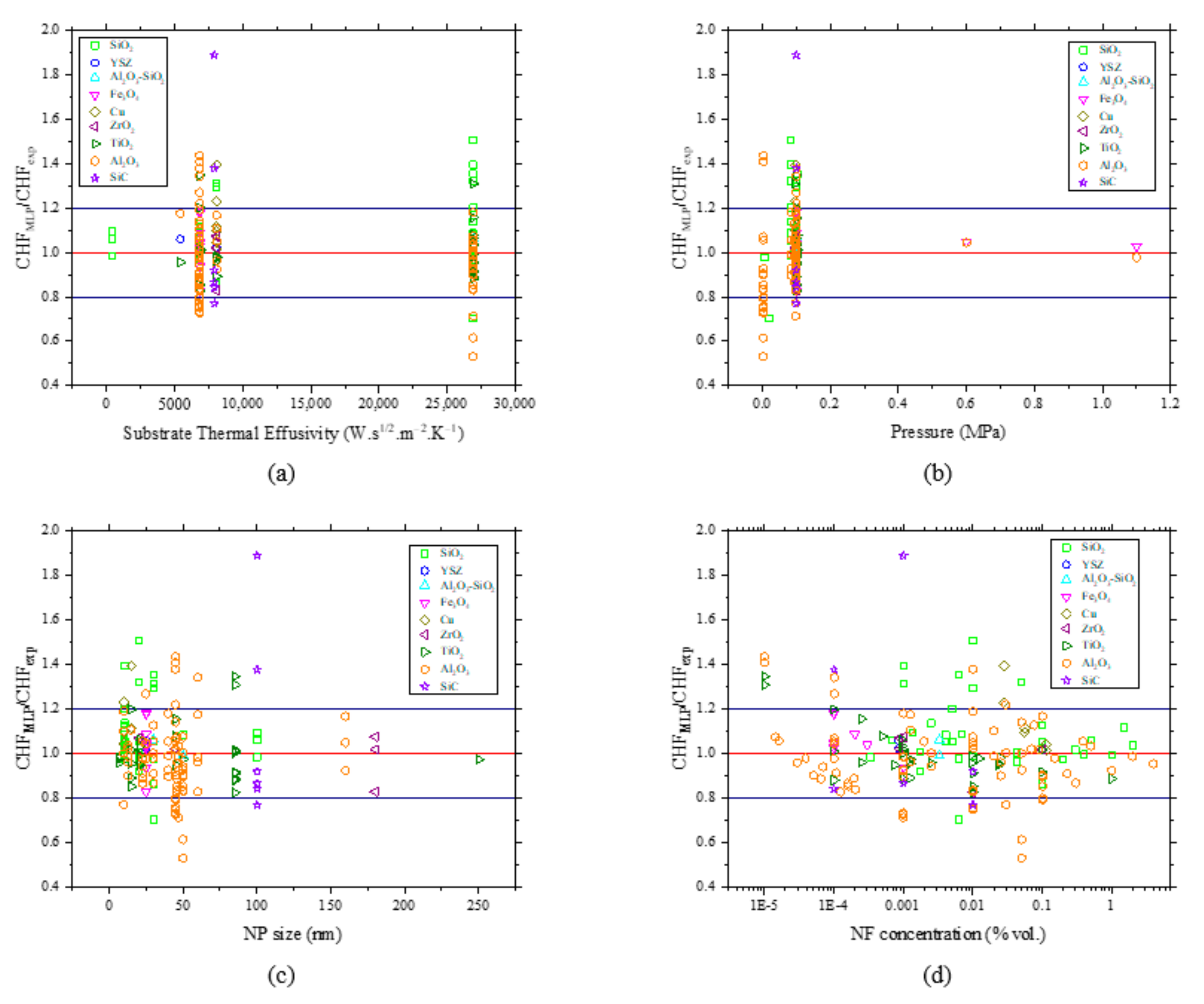
Figure 22 presents the CHF ratio between the predictions and the experimental data for all the database NPs and each feature.

In Figure 22, it can be observed that the CHF NP ratio is predominantly in a $\pm$20% range, covering around 81% of the datapoints, with a few scattered data reaching the $\pm$50% range. Figure 22a,b do not present very dispersed data. In fact, only a small number of substrates were used in all the experiments, while most of the studies performed atmospheric pressure NF pool boiling experiments. It also shows that the predictions were not biased toward any specific NP, which emphasizes the fact that the MLP model can be a powerful tool to predict the CHF in NF pool boiling experiments.

6. Conclusions

The present study aimed to create an improved model that can accurately predict NF pool boiling CHF, which cannot currently be predicted by any other empirical or theoretical models due to the complexity of this phenomenon. In order to achieve this goal, an NF pool boiling database was constructed by compiling experimental data from the literature, and this database was used to train three ML models—SVR, MLP, and RF—which had their performances analyzed and compared. A systematic method to build three ML models was presented to create a generalized model without overfitting that could add to the understanding of CHF in NF pool boiling.

It is important to highlight that the database was constructed based on published experimental data; this construction involves large uncertainties being associated with the data. Many challenges were addressed during the construction of the database, such as (1) lack of information: some studies do not provide full information on the experiments, conditions, material, dimensions, etc., and (2) lack of a pattern for data display: some papers highlight the CHF points in the plots, while others display the ratio between NF, CHF, and base fluid CHF, but never the CHF itself.

Despite the large degree of uncertainty related to the database construction, the results showed that the ML models predicted NF boiling CHF quite well, capturing the main physical mechanism of the process. The best SVR fitting obtained a testing score of 84%, while the best MLP fitting obtained a testing score of 87%, and finally, the best RF fitting obtained a testing score of 90%. Nevertheless, it is widely recognized that a larger database can yield improved fittings for machine learning (ML) models, resulting in more accurate predictions. Although all three developed ML models presented good results, the SVR model presented limited results, with the lowest mean R² testing score. The RF model presented very good results; however, its mean R² testing score was lower than that of the MLP model, which indicates a higher variability in the 10-run testing. Hence, the MLP model presented the best results overall, with the highest mean R² testing score and the lowest variability in the 10-run testing.

Furthermore, all three developed ML models were used to deeply understand and discuss the effect of each CHF feature, i.e., pressure, substrate thermal effusivity, NP thermal effusivity, NP size, and NF concentration, on NF pool boiling. Three feature importance evaluation tools were also applied to the data to quantify and rank each feature’s importance in relation to NF pool boiling CHF. All three models agreed that among the selected importance features, the pressure was the most relevant, followed by the NP size, while substrate thermal effusivity was considered to not have a significant effect on NF pool boiling CHF. The combined effect between pressure and NP deposition is also relevant in the process due to its impact on bubble size, nucleation sites, and nucleation frequency.

Lastly, the MLP model was then applied to generate CHF predictions for all of the 170 datapoints from the constructed database. Those predictions were compared to the experimental data and Kandlikar’s model. As expected, the MLP predictions proved to be more accurate.

As a result of this study, ML models hold significant promise as effective tools for addressing non-linear problems, including the characterization of CHF in NF pool boiling, as demonstrated in the work.