Optimized Power Flow Control to Minimize Congestion in a Modern Power System

Abstract

The growing integration of renewable energy sources (RES) into the power system causes congestion to occur more frequently. In order to reduce congestion in the short term and to make the utilization of the power system more efficient in the long term, power flow control (PFC) in the transmission system has been proposed. However, exemplary studies show that congestion will increase also in the distribution system if the transmission system is expanded. For this reason, the potential of PFC to reduce congestion in a model of a real 110 kV distribution system is investigated. Several Unified Power Flow Controller (UPFC) devices are optimized in terms of their number and placement in the power system, their size, control parameters, and costs, by using a Parallel Tempering approach as well as a greedy algorithm. Two optimization variants are considered, one reducing the number of degrees of freedom by integrating system knowledge while the other does not. It is found that near a critical grid state and disregarding costs, PFC can reduce congestion significantly (99.13%). When costs of the UPFCs are taken into account, PFC can reduce congestion by 73.2%. A basic economic analysis of the costs reveals that the usage of UPFCs is profitable. Furthermore, it is found that the reduction in the solution space of the optimization problem leads to better results faster and that, contrary to expectations, the optimization problem is simple to solve. The developed methods allow not only for the determination of the optimal use of UPFCs to minimize congestion, but also to estimate their profitability.

1. Introduction

Due to the growing share of renewable energy sources (RES) in combination with its volatile nature, congestion in the power system, i.e., violations of voltage or thermal limits of grid elements, may occur more frequently [1]. The increase in RE curtailment in Germany in recent years highlights this problem. To ensure secure grid operation, the demand of curtailment went up from $555 \mathrm{G}\mathrm{W}\mathrm{h}$ in 2013 to $5402.7 \mathrm{G}\mathrm{W}\mathrm{h}$ in 2018 [2]. According to §15(2) in the German Renewable Energy Act (Erneuerbare-Energien-Gesetz, EEG), the associated costs of estimated USD 183 m in 2014 and USD 635 m in 2018 can be translated by grid operators into grid fees, resulting in high costs for society [2] (p. 161). To avoid these costs, the expansion of the power system plays a crucial role. However, several studies show that grid expansion and reinforcement alone is not an efficient solution to avoiding congestion both at distribution system level (110 kV) [3] and at transmission system level (220 kV) [4]. For this reason, the investigation of congestion management approaches is important to ensure a secure and efficient operation of the power system in the future.

In this paper, congestion management by means of power flow control (PFC) is investigated, as this approach comes with a number of advantages. In contrast to market-based approaches, where agreements between the grid operator and, e.g., flexible generators or consumers are necessary, no additional agreements are needed for PFC, as the grid operator directly controls the required resources. Furthermore, since PFC redirects power flows from heavily loaded lines to those with lower loads, a higher transmission capacity of the power system is achieved. The increased transmission capacity comes without the need to build new lines, which is another advantage of the technology, as this is of great interest for the public [5]. It should be noted that, for PFC to be effective, free transmission capacities must be available in parts of the power system and that the use of PFC causes additional losses when power flows no longer adjust by means of the least resistance. Nonetheless, the literature recommends the use of PFC and refers to an implementation in the transmission system. It is argued that PFC can be implemented faster than grid expansion and can thus reduce congestion in the near future [6] (p. 4). Moreover, in the long term, PFC should be taken into account in both the expansion planning and operation of the power system, as it enables a more efficient use of it [6] (p. 20).

Recommending PFC in the transmission system seems reasonable, since, in 2018, 86.8% of the demand for curtailment occurred in the transmission system and 13.2% of it occurred in the distribution system [7] (p. 34). However, exemplary studies show that congestion within the distribution system will increase if the transmission system is expanded [8]. For this reason, the question arises whether the use of PFC should also be considered in the distribution system.

The aim of this work is, therefore, to determine the potential of PFC to minimize congestion in a 110 kV distribution system. To achieve this goal, this work aims to find, by computer simulations [9], an optimized configuration [10,11] of several Unified Power Flow Controller (UPFC) devices that minimizes congestion in the distribution system while taking into account capital costs. In addition, by neglecting the costs, the maximum potential of PFC to reduce congestion is evaluated. While optimizing, the focus is not on the permanent operation of the UPFCs, but more on their arrangement. With regard to a permanent operation of UPFCs, various methods can be found in the literature [12]. In [13,14,15], optimization is carried out with regard to the number, placement in the power system, size, control parameters, and costs of the UPFCs. In [13], exhaustive search is applied to maximize social welfare, and the authors in [14,15] apply particle swarm optimization and a genetic algorithm to maximize system loadability. This work extends the existing research by optimizing the number, placement, size, control parameters, and costs of the UPFCs to minimize congestion in the power system. To do so, this work applies the convenient and efficient Parallel Tempering approach and a greedy algorithm. In comparison to the literature, this work not only states the costs of a proposed UPFC application, but also relates them to the costs of the saved demand of curtailment.

One of the major contributions of this study is the proposal of two optimization variants, where in one case the number of degrees of freedom is reduced by integrating knowledge of the power system. As an example, the placement of UPFCs is no longer considered on all lines, but only on congested lines. Another major contribution is the further development of the Power Injection Model (PIM), which is used to model the UPFC. Not only is it explained how the PIM can be properly interpreted, but a calculation method for the series transformer reactance is also provided. Moreover, an analytical approach is developed that enables one to determine the allowed control parameters of a UPFC with respect to its operating limits in advance, replacing the iterative approach proposed in the literature [16].

The developed methods allow one to identify an optimized UPFC application that minimizes congestion in a power system. By quantifying the reduction in congestion and calculating the remaining demand of curtailment, the potential of PFC to integrate more RE is demonstrated.

The remainder of the paper is structured as follows. At the beginning of Section 2, it is explained why the UPFC is used for PFC in this work, and the PIM is depicted. Then, the developed methods and optimization algorithms are outlined. In Section 3, the results of this work are presented. The paper concludes with a summary of the most important findings and an outlook on possible future research.

2. Methods and Materials

The methods and materials used in this work are introduced in this section. Firstly, the choice of the PFC device (UPFC) and the reasons for describing it using the PIM are justified (Section 2.1 and Section 2.2). Important modeling aspects concerning UPFCs and the PIM are then discussed, leading to the formulation of the full optimization problem in Section 2.7. The Metropolis algorithm and the Parallel Tempering approach are introduced next (Section 2.9 and Section 2.10). Finally, the grid model is introduced in Section 2.11. A comprehensive approach to the following methods can be found in the thesis [17].

2.1. Choice of Power Flow Control Device

According to [18], resolving congestion depends on changing the line resistance R, which is not considered in this work, and the current of a line [18] (p. 250),

$$\tilde{I}=\frac{V_{\mathrm{i}}\cos \delta +j{V}_{\mathrm{i}}\sin \delta -V_{\mathrm{f}}}{jX}.$$

(1)

Here, the tilde indicates whether the entity is complex, and $V_{\mathrm{i}}$ and $V_{\mathrm{f}}$ are the voltage magnitudes of the initial bus and of the terminal bus of the line, respectively. The angle between the two phasors ${\tilde{V}}_{\mathrm{i}}$ and ${\tilde{V}}_{\mathrm{f}}$ is $\delta$, where ${\tilde{V}}_{\mathrm{i}}$ is set as a reference phasor with angle 0. The impedance of the line is $jX$, with j as the imaginary unit. All entities in this work describe three phase entities if not marked explicitly.

The question is whether changing one of the variables is superior to changing one of the others in order to resolve congestion. The literature addresses this question and introduces the maximum system loadability. It is defined as the maximum amount of power that the grid can supply without overloaded lines and with acceptable voltage levels, if all loads and active power of the generators (e.g., RE) are iteratively increased in the same ratio. It turns out that combining different Flexible AC Transmission Systems (FACTSs) regulating different variables results in a higher maximum system loadability [19]. The maximum system loadability is a comparable measure for the objectives of this work. It is therefore assumed that, in order to carry out the most effective PFC, different variables should be changed on different lines. The Unified Power Flow Controller FACTS device can control $V_{\mathrm{i}}$, $V_{\mathrm{f}}$, X, and $\delta$ individually or simultaneously. The question of whether a combination of variables should be changed per line does not need to be investigated, since, with the following optimization, a simultaneous change in the variables will result if it is advantageous. The authors are aware that there are other devices for PFC in addition to the UPFC. 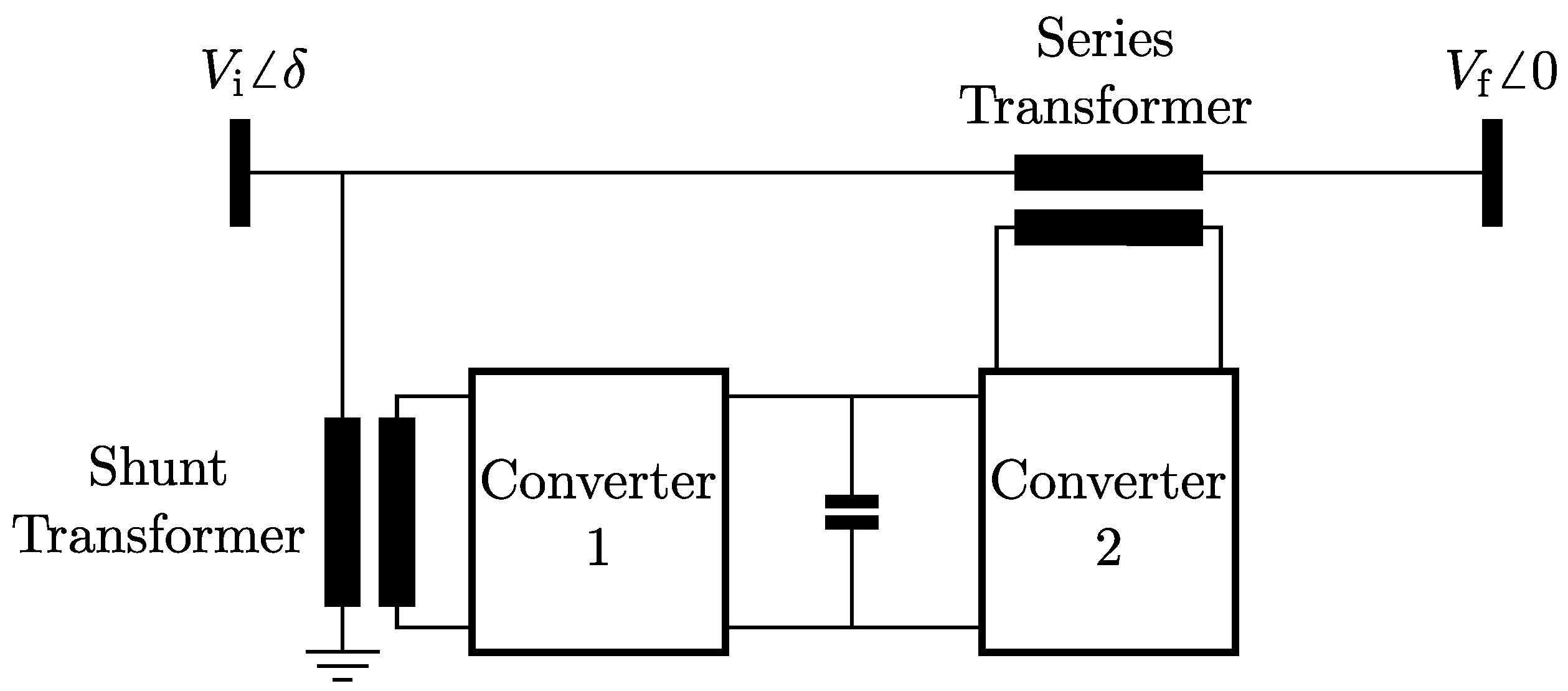However, for the above reason, and taking into account the comparison of different FACTS devices in [15,19], the UPFC is selected as the most suitable device to determine the maximum potential of PFC. The basic setup of a UPFC is depicted in Figure 1.

A series transformer is connected to the line in series, and a shunt transformer is connected to the initial bus of the line or to the line itself. The AC/DC converters are connected via a DC link [16].

2.2. Power Injection Model of UPFC

Among the many different models available for UPFCs, the PIM according to [16] is chosen because it can be easily integrated into stationary power flow analysis. The derivation of the PIM is based on the main functionality of the UPFC, namely, the series voltage source injection on the line. The series voltage source can be controlled in magnitude and phase:

$${\tilde{V}}_{\mathrm{se}}=r {\tilde{V}}_{\mathrm{i}} e^{j\gamma },$$

(2)

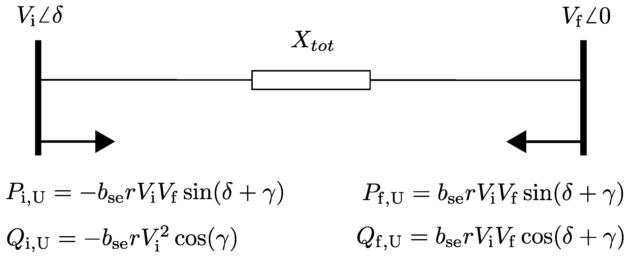
where $r\in [0,r_{max}]$ and $\gamma \in [0°,360°]$ are the control parameters of the UPFC [16]. The basic idea of the PIM is to represent the functionality of a UPFC by additional load and generation at the buses of the line. The model is depicted in Figure 2. Here, $P_{\mathrm{i},\mathrm{U}}$ is the active power, and $Q_{\mathrm{i},\mathrm{U}}$ is the reactive power injection at the initial bus of the line. $P_{\mathrm{f},\mathrm{U}}$ and $Q_{\mathrm{f},\mathrm{U}}$ are at the terminal bus. In the following two subsections, it is discussed whether P and Q represent load or generation, and $b_{\mathrm{se}}$ is determined.

2.3. Interpretation of the Power Injection Model

To identify whether the expressions in Figure 2 represent load or generation, the series voltage source is again considered. If it is placed at the beginning of the line, the voltage on the line after the series voltage source is

$${\tilde{V}}_{\mathrm{i}}^{\prime }={\tilde{V}}_{\mathrm{se}}+{\tilde{V}}_{\mathrm{i}} .$$

(3)

The apparent power at the terminal bus of the line can then be expressed as

$$\begin{array}{cc}{\tilde{S}}_{\mathrm{f}}={\tilde{V}}_{\mathrm{f}}{\tilde{I}}^{*}\hfill & = {\tilde{V}}_{\mathrm{f}}{\left[\frac{{\tilde{V}}_{\mathrm{i}}^{\prime }-{\tilde{V}}_{\mathrm{f}}}{j{X}_{\mathrm{tot}}}\right]}^{*}={\tilde{V}}_{\mathrm{f}}{\left[\frac{{\tilde{V}}_{\mathrm{se}}+{\tilde{V}}_{\mathrm{i}}-{\tilde{V}}_{\mathrm{f}}}{j{X}_{\mathrm{tot}}}\right]}^{*}=\hfill \\ \hfill & V_{\mathrm{f}}\left[\frac{V_{\mathrm{i}}(\sin \delta +r\sin (\delta +\gamma )+j\cos \delta +jr\cos (\delta +\gamma ))-j{V}_{\mathrm{f}}}{X_{\mathrm{tot}}}\right]\hfill \end{array}$$

(4)

with

$$X_{\mathrm{tot}}=X_{\mathrm{line}}+X_{\mathrm{se}},$$

(5)

where $X_{\mathrm{line}}$ is the reactance of the line, and $X_{\mathrm{se}}$ denotes the reactance of the series transformer, which is determined in the next section. For the active power at the receiving bus and for $\gamma =90°$, it follows that

$$P_{\mathrm{f}}=\frac{V_{\mathrm{i}}{V}_{\mathrm{f}}}{X_{\mathrm{tot}}}\sin \delta +\frac{r{V}_{\mathrm{i}}{V}_{\mathrm{f}}}{X_{\mathrm{tot}}}\sin (\delta +\gamma )=\frac{V_{\mathrm{i}}{V}_{\mathrm{f}}}{X_{\mathrm{tot}}}\left(\sin \delta +r\cos \delta \right),$$

(6)

where

$$\sin (\delta +\gamma )=\sin \delta \cos \gamma +\cos \delta \sin \gamma$$

(7)

is used. In [18] (p. 251), the active power of a line without additional series voltage source at the terminal bus is determined as

$$P_{\mathrm{f}}=\frac{V_{\mathrm{i}}{V}_{\mathrm{f}}}{X_{\mathrm{tot}}}\sin \delta .$$

(8)

Equation (6) thus shows that, for $\gamma =90°$ and for small $\delta$, both positive and negative, the power at the receiving bus is increased by using a series voltage source. To model an increase in $P_{\mathrm{f}}$ by additional power injections, $P_{\mathrm{i},\mathrm{U}}$ and $P_{\mathrm{f},\mathrm{U}}$ in Figure 2 must be interpreted as loads, because, for $\gamma =90°$ and for small $\delta$, both positive and negative, they then represent an additional generation at the initial bus and an additional load at the terminal bus, which leads to an increase in $P_{\mathrm{f}}$. Thus, interpreting the equations in Figure 2 as loads ensures correct modeling in accordance with (6). This interpretation is in contrast to [16], where $\gamma =90°$ corresponds to a decrease in the active power flow along the line.

2.4. Calculation of the Reactance in the Power Injection Model

In Figure 2, $b_{\mathrm{se}}$ is determined as follows:

$$b_{\mathrm{se}}=\frac{1}{X_{\mathrm{tot}}}=\frac{1}{X_{\mathrm{line}}+X_{\mathrm{se}}},$$

(9)

where $X_{\mathrm{line}}$ can be regarded as given. The reactance $X_{\mathrm{se}}$ of the series transformer, which is regarded as lossless, is represented by the short circuit reactance [20]

$$X_{\mathrm{k}}=X_{\mathrm{se}}=u_{\mathrm{k}}\frac{\left|{\tilde{V}}_{\mathrm{N},\mathrm{a}}\right|}{\left|{\tilde{I}}_{\mathrm{N},\mathrm{a}}\right|}.$$

(10)

Here, $u_{\mathrm{k}}=0.1$ is used in accordance with [21] (p. 2) and [20] (p. 17). Index a indicates single phase entities, such as ${\tilde{I}}_{\mathrm{N},\mathrm{a}}$ as the rated current and ${\tilde{V}}_{\mathrm{N},\mathrm{a}}$ as the rated voltage of the series transformer. The latter is set to equal the maximum voltage magnitude that Converter 2 can supply, according to (2).

$$\left|{\tilde{V}}_{\mathrm{N},\mathrm{a}}\right|=\left|r_{\max }{\tilde{V}}_{\mathrm{i},\mathrm{a}}{e}^{j\gamma }\right|=r_{\max }\frac{\left|{\tilde{V}}_{\mathrm{i}}\right|}{\sqrt{3}}=r_{\max }\frac{\left|{\tilde{V}}_{\mathrm{grid}}\right|}{\sqrt{3}}.$$

(11)

The simplification $\left|{\tilde{V}}_{\mathrm{i}}\right|=\left|{\tilde{V}}_{\mathrm{grid}}\right|=110 \mathrm{k}\mathrm{V}$ is appropriate, since the bus voltages encountered in this work are close to 110 kV. Furthermore, it follows that

$$\left|{\tilde{I}}_{\mathrm{N},\mathrm{a}}\right|=\frac{1}{3}\left|{\left(\frac{{\tilde{S}}_{\mathrm{N}}}{{\tilde{V}}_{\mathrm{N},\mathrm{a}}}\right)}^{*}\right|=\frac{1}{3}\left|\frac{{\tilde{S}}_{\mathrm{N}}}{{\tilde{V}}_{\mathrm{N},\mathrm{a}}}\right|=\frac{1}{3}\frac{\left|{\tilde{S}}_{\mathrm{se}}\right|}{\left|{\tilde{V}}_{\mathrm{N},\mathrm{a}}\right|},$$

(12)

with $\left|{\tilde{S}}_{\mathrm{N}}\right|=\left|{\tilde{S}}_{\mathrm{se}}\right|$ as the rated power of the series transformer. Inserting (11) and (12) into (10) yields

$$X_{\mathrm{se}}=u_{\mathrm{k}}{r}_{\max }^2\frac{{\left|{\tilde{V}}_{\mathrm{grid}}\right|}^2}{\left|{\tilde{S}}_{\mathrm{se}}\right|}.$$

(13)

$\left|{\tilde{S}}_{\mathrm{se}}\right|$ can be taken as given, since the optimization dictates it. Finally, in order to calculate $X_{\mathrm{se}}$, $r_{\max }$ must be specified. Next, it is shown that $r_{\max }=r_{\max }\left(\left|{\tilde{S}}_{\mathrm{se}}\right|\right)$ and can therefore not be chosen arbitrarily.

2.5. Operational Limits of Unified Power Flow Controllers

The operational limits of a UPFC can be expressed in terms of the rated powers $\left|{\tilde{S}}_{\mathrm{C}1}\right|$ and $\left|{\tilde{S}}_{\mathrm{C}2}\right|$ of its converters

$$\begin{array}{c}\hfill \sqrt{P_{\mathrm{C}1}^2+Q_{\mathrm{C}1}^2}\le \left|{\tilde{S}}_{\mathrm{C}1}\right|\\ \hfill \sqrt{P_{C2}^2+Q_{\mathrm{C}2}^2}\le \left|{\tilde{S}}_{\mathrm{C}2}\right|,\end{array}$$

(14)

where Index C1 indicates Converter 1 and Index C2 indicates Converter 2. It is assumed that the rated power of the converters is equal and that the UPFC transformers have the same rated power:

$$\left|{\tilde{S}}_{\mathrm{C}1}\right|=\left|{\tilde{S}}_{\mathrm{C}2}\right|=\left|{\tilde{S}}_{\mathrm{sh}}\right|=\left|{\tilde{S}}_{\mathrm{se}}\right|$$

(15)

with $\left|{\tilde{S}}_{\mathrm{sh}}\right|$ as the rated power of the shunt transformer. As the UPFC cannot generate or absorb active power, $P_{\mathrm{C}1}=-P_{\mathrm{C}2}$ must hold. In [16], regarding the PIM, it is assumed that $Q_{\mathrm{C}1}=0$. With (15), (14) simplifies to

$$\sqrt{P_{\mathrm{C}2}^2+Q_{\mathrm{C}2}^2}\le \left|{\tilde{S}}_{\mathrm{se}}\right|.$$

(16)

In the following, $\left|{\tilde{S}}_{\mathrm{se}}\right|$ is referred to as the size of the UPFC. In [16], the active power and reactive power of Converter 2 are determined as

$$\begin{array}{cc}\hfill P_{\mathrm{C}2}& =b_{\mathrm{se}}r{V}_{\mathrm{i}}{V}_{\mathrm{f}}\sin (\delta +\gamma )-b_{\mathrm{se}}r{V}_{\mathrm{i}}^2\sin \left(\gamma \right)\hfill \\ \hfill Q_{\mathrm{C}2}& =-b_{\mathrm{se}}r{V}_{\mathrm{i}}{V}_{\mathrm{f}}\cos (\delta +\gamma )+b_{\mathrm{se}}r{V}_{\mathrm{i}}^2\cos \left(\gamma \right)+b_{\mathrm{se}}{r}^2{V}_{\mathrm{i}}^2.\hfill \end{array}$$

(17)

Inserting this into (16) and applying (9) yields

$$\begin{array}{cc}{\left(\frac{r}{u_{\mathrm{k}}{r}^2{\left|{\tilde{V}}_{\mathrm{grid}}\right|}^2+\left|{\tilde{S}}_{\mathrm{se}}\right|X}\right)}^2\hfill & [V_{\mathrm{i}}^2{V}_{\mathrm{f}}^2+V_{\mathrm{i}}^4-\hfill \\ \hfill & \hfill 2V_{\mathrm{i}}^3{V}_{\mathrm{f}}(\sin (\delta +\gamma )& \sin \left(\gamma \right)+\cos (\delta +\gamma )\cos \left(\gamma \right))-\hfill \\ \hfill & \hfill & 2r{V}_{\mathrm{i}}^3{V}_{\mathrm{f}}\cos (\delta +\gamma )+2r{V}_{\mathrm{i}}^4\cos \left(\gamma \right)+r^2{V}_{\mathrm{i}}^4]\le 1,\hfill \end{array}$$

(18)

where $r_{\max }$ in (13) is set as equal to r in order to determine for which values of r and $\gamma$ the expression is satisfied. At this point, $r_{\max }$ is defined as the maximum value of r, which fulfills the above inequality for $0°\le \gamma \le 360°$. By deploying this $r_{\max }$, the operational limits of the UPFC are never violated for any value of $\gamma$. It follows that, before applying the PIM, a UPFC size $\left|{\tilde{S}}_{\mathrm{se}}\right|$ must be chosen, from which $r_{\max }\left(\left|{\tilde{S}}_{\mathrm{se}}\right|\right)$ is determined to calculate $X_{\mathrm{se}}$.

Figure 3 illustrates the left-hand side of (18) for an exemplary line with $V_{\mathrm{i}}=110 \mathrm{k}\mathrm{V}$, $V_{\mathrm{f}}=109 \mathrm{k}\mathrm{V}$, $\delta =4°$, and $X=5 \Omega$. Three different power ratings of the series transformers are considered. For a 10 MVA series transformer, the grey line in the figure represents $r_{\max }(10 \mathrm{MVA})$. It can be seen that values of $r\le r_{\max }$ also fulfill the inequality.

For the following investigations, (18) is evaluated for each line in the 110 kV distribution system, for the series transformer power ratings appearing in this work $\left|{\tilde{S}}_{\mathrm{se}}\right|\in \left\{1 \mathrm{MVA},2 \mathrm{MVA},\dots ,100 \mathrm{MVA}\right\}$ and for 1000 steps each in $r\in [0.01, 0.3]$ and $\gamma \in [0°, 360°]$.

2.6. Optimization of UPFC Configuration

If more than one UPFC is to be installed in a power system, several questions arise. The number of UPFCs, the placement in the power system, the size of the devices, and the control parameters r and $\gamma$ cannot be determined trivially. Therefore, optimization is carried out, and two optimization approaches are developed.

First, for a restricted optimization denoted as $O_{\mathrm{sys}}$, the number of UPFCs and their size will be determined by means of optimization; see also

Table 1. Overview of optimization variants. For $n_{\mathrm{pos}}$ and $n_{\mathrm{pos}}^{\mathrm{sys}}$ refer to Section 2.8.

Variant	${\mathit{O}}_{\mathbf{sys}}$	${\mathit{O}}_{+}$
Degrees of freedom	Number of UPFCs $n_{\mathrm{upfcs}}$	Number of UPFCs $n_{\mathrm{upfcs}}$
	Sizing $\left|{\tilde{S}}_{\mathrm{se}}\right|$	Sizing $\left|{\tilde{S}}_{\mathrm{se}}\right|$
	Placement: Only congested lines $n_{\mathrm{pos}}^{\mathrm{sys}}$	Placement: All $n_{\mathrm{pos}}$ lines
	Control parameters r, $\gamma$	Control parameters r, $\gamma$
Constraints	$r=r_{\max }$	$r\in [0,r_{\max }]$
	$\delta +\gamma \in \{90°,270°\}$	$\gamma \in [0°,360°]$
	$n_{\mathrm{upfcs}}\le n_{\mathrm{pos}}^{\mathrm{sys}}$	$n_{\mathrm{upfcs}}\le n_{\mathrm{pos}}$
	$\left|{\tilde{S}}_{\mathrm{se}}\right|\in \left\{1,2,\dots ,100\right\}\mathrm{MVA}$	$\left|{\tilde{S}}_{\mathrm{se}}\right|\in \left\{1,2,\dots ,100\right\}\mathrm{MVA}$

. For the placements, only congested lines are considered, and $r=r_{\max }\left(\left|{\tilde{S}}_{\mathrm{se}}\right|\right)$ is specified. Together with $\delta +\gamma \in \{90°, 270°\}$, the active power flow of the lines is minimized in this approach. In order to ensure a cost-efficient use of the UPFCs, costs are optimized as well. This optimization variant integrates knowledge of the power system’s lines and the UPFCs’ operation.

For a more comprehensive optimization denoted as $O_{+}$, all lines of the power system and control parameters of $r\in [0, r_{\max }]$ and $\gamma \in [0°, 360°]$ are considered for a UPFC installation.

2.7. Objective Function

For the optimized power system integration of UPFCs, an objective function is defined. The summation of two terms, with $F_{\mathrm{c}}$ describing the costs of a UPFC configuration and $F_{\mathrm{vio}}$ quantifying congestion in the grid model, yields for the objection function

$$F=F_{\mathrm{c}}+F_{\mathrm{vio}}=\underset{F_{\mathrm{c}}}{\underbrace{\sum _{i=1}^{n_{\mathrm{upfcs}}}{C}_{\mathrm{upfc},i}}}+\underset{F_{\mathrm{vio}}}{\underbrace{\phantom{{\sum }_{i=1}^{n_{upfcs}}}{\omega }_{\mathrm{vio}}L}}.$$

(19)

Here, $C_{\mathrm{upfc},i}$ describes the investment costs of UPFC i according to [22]:

$$C_{\mathrm{upfc}}=(\frac{0.3 \$}{{\mathrm{MVA}}^3}{\left|{\tilde{S}}_{\mathrm{se}}\right|}^2-\frac{269.1 \$}{{\mathrm{MVA}}^2}\left|{\tilde{S}}_{\mathrm{se}}\right|+\frac{188,200 \$}{\mathrm{MVA}})\left|{\tilde{S}}_{\mathrm{se}}\right| ,$$

(20)

where $n_{\mathrm{upfcs}}$ is the number of UPFCs added to the distribution system, and ${\omega }_{\mathrm{vio}}$ is the weighting factor of L. The function L maps the violations of voltage and thermal limits of the grid elements, i.e., the occurrences of congestion. It is defined as

$$L=\sum _{j=1}^{n_{\mathrm{lines}}}{L}_{\mathrm{line},j}+\sum _{k=1}^{n_{\mathrm{buses}}}{L}_{\mathrm{bus},k},$$

(21)

with $n_{\mathrm{lines}}$ as the number of lines and $n_{\mathrm{buses}}$ as the number of buses in the power system. $L_{\mathrm{line}}$ maps each violation of the thermal limit of a line and is defined as

$$L_{\mathrm{line}}=\{\begin{array}{cc}0\hfill & ;\mathrm{if} l_{\mathrm{loading}}\le 100\%\hfill \\ {\omega }_{\mathrm{line}}\left(\frac{l_{\mathrm{loading}}-100}{100}\right)\hfill & ;\mathrm{else},\hfill \end{array}$$

(22)

where $l_{\mathrm{loading}}$ is the loading of the line in %, and ${\omega }_{\mathrm{line}}$ is a weighting factor. The above equation is divided and subtracted by 100 to obtain comparable values with respect to $L_{\mathrm{bus}}$. The latter describes the extent to which the violation of a single bus voltage limit contributes to L and is defined as

$$L_{\mathrm{bus}}=\{\begin{array}{cc}0\hfill & ;\mathrm{if} 0.9 \mathrm{p}.\mathrm{u}.\le V_{\mathrm{bus}}\le 1.1 \mathrm{p}.\mathrm{u}.\hfill \\ {\omega }_{\mathrm{bus}}\left(\right|1-V_{\mathrm{bus}}|-0.1)\hfill & ;\mathrm{else},\hfill \end{array}$$

(23)

where $V_{\mathrm{bus}}$ is the voltage magnitude of a bus given in p.u. The violation of a bus voltage limit can be weighted with ${\omega }_{\mathrm{bus}}$. This type of steady-state voltage constraint covers only one aspect of power quality and is considered as such by comparable works in the literature [23].

Throughout the work, ${\omega }_{\mathrm{line}}=1$ and ${\omega }_{\mathrm{bus}}=5$ are set. This allows the investigations to focus on line congestion, as, with these weighting factors, bus voltage violations are less likely compared to thermal limit violations. In fact, no violations of bus voltages were observed in the results. ${\omega }_{\mathrm{vio}}={10}^8$ is set across the work, so that $F_{\mathrm{c}}$ is in the same order of magnitude as $F_{\mathrm{vio}}$. For a better handling, the objective function is scaled:

$$F:=F/{10}^6.$$

(24)

2.8. Configuration of Unified Power Flow Controllers

The subsequent optimization algorithms start with a random initial configuration of UPFCs. First, the initial number of UPFCs $n_{\mathrm{upfcs}}$ is to be determined. It is important to note that not all of the lines of the power system can necessarily be occupied by a UPFC. If, for a certain line and for all possible sizes of a UPFC, no $r_{\max }$ in (18) can be found, the line cannot be used for a UPFC installation. The maximum number of lines that can be considered is denoted as $n_{\mathrm{pos}}$. The number of UPFCs in the initial configuration $n_{\mathrm{upfcs}}$ is therefore chosen randomly from $\{1,2,\dots ,n_{\mathrm{pos}}\}$ for the optimization $O_{+}$. In the optimization $O_{\mathrm{sys}}$, the number of lines that can be considered is further limited to congested lines. In this case, the number of applicable lines is denoted as $n_{\mathrm{pos}}^{\mathrm{sys}}\le n_{\mathrm{pos}}$ and it holds that $n_{\mathrm{upfcs}}$ is randomly chosen from $\{1,2,\dots ,n_{\mathrm{pos}}^{\mathrm{sys}}\}$.

Finally, each UPFC i for $i\in \{1,\dots ,n_{\mathrm{upfcs}}\}$ is assigned randomly to a line $x_i$ and a size $S_i$. For the $O_{+}$ optimization, a value $r_i$ is chosen from $[0,r_{\max }]$, and a value ${\gamma }_i$ is chosen from $\{0°,\dots ,360°\}$, with ${\gamma }_i$ being a natural number.

Let C be a configuration of UPFCs, which is modified to $C^{\prime }$:

$$C=\left[\begin{array}{cccc}{x}_1& S_1& r_1& {\gamma }_1\\ ⋮& ⋮& ⋮& ⋮\\ x_{\mathrm{n}\mathrm{upfcs}}& S_{\mathrm{n}\mathrm{upfcs}}& r_{\mathrm{n}\mathrm{upfcs}}& {\gamma }_{\mathrm{n}\mathrm{upfcs}}\end{array}\right]\}{n}_{\mathrm{upfcs}}\to$$

$$C^{\prime }=\left[\begin{array}{cccc}{x}_1^{\prime }& S_1^{\prime }& r_1^{\prime }& {\gamma }_1^{\prime }\\ ⋮& ⋮& ⋮& ⋮\\ x_{\mathrm{n}\prime \mathrm{upfcs}}^{\prime }& S_{\mathrm{n}\prime \mathrm{upfcs}}^{\prime }& r_{\mathrm{n}\prime \mathrm{upfcs}}^{\prime }& {\gamma }_{\mathrm{n}\prime \mathrm{upfcs}}^{\prime }\end{array}\right]\}{n}_{\mathrm{upfcs}}^{\prime }$$

During the optimization process from a given current configuration, trial configurations are created by random changes, which might become the next current configuration. $C^{\prime }$ variables indicated with a dash are changed with a probability according to

Table 2. Modification of the UPFC configuration. H is chosen randomly from $\{-1,1\}$.

Variables	Probability p	Variables Change with Increment $\mathbf{\Delta }$
$n_{\mathrm{upfcs}}$	$p_{\mathrm{upfcs}}$	$n_{\mathrm{upfcs}}^{\prime }=n_{\mathrm{upfcs}}+{\Delta }_{\mathrm{upfcs}}H$
$S_i$	$p_S$	$S_i^{\prime }=S_i+{\Delta }_{S}H$
$r_i$	$p_{\mathrm{r}}$	$r_i^{\prime }=r_i+{\Delta }_{\mathrm{r}}H$
${\gamma }_i$	$p_{\gamma }$	${\gamma }_i^{\prime }={\gamma }_i+{\Delta }_{\gamma }H$

. The table does not describe direct changes to the UPFC positions, but changes to the number $n_{\mathrm{upfcs}}$ of UPFC. This effectively allows for UPFC installations on changing lines, since, for $n_{\mathrm{upfcs}}^{\prime }>n_{\mathrm{upfcs}}$, new UPFCs at randomly chosen unoccupied lines are added to the configuration, and, for $n_{\mathrm{upfcs}}^{\prime }<n_{\mathrm{upfcs}}$, $n_{\mathrm{upfcs}}-n_{\mathrm{upfcs}}^{\prime }$, UPFCs are deleted randomly from C. Within the $O_{\mathrm{sys}}$ variant, $r_i$ and ${\gamma }_i$ are only changed with new UPFCs added to the configuration.

2.9. Metropolis Algorithm and Optimization

In [14], a genetic algorithm and particle swarm optimization are used to optimize the variant $O_{+}$. Such algorithms, which are inspired by optimization processes performed in nature, are characterized by several parameters such as population sizes, mutation probabilities, or particle properties, which have to be suitably selected within many trial runs. Therefore, a physical viewpoint is employed in the present work. It is based on the fact that any system in contact with a heat bath with temperature T will approach its ground state, i.e., the minimum energy, if the temperature is lowered $T\to 0$. This was transferred into an optimization algorithm by the Simulated Annealing approach [24], where the function to be optimized is taken as energy of a system. The Metropolis algorithm [25] is used to simulate the system, which is subject to lower and lower temperatures, therefore approaching the lowest energy. Still, the dynamics might be caught in local minima. This can be avoided when a generalization, the Parallel Tempering [26,27], is applied, which is based on simulating the system at several temperatures in parallel and allowing for moving up and down the temperature space (see Section 2.10 for details). In this way, a much simpler implementation is obtained as compared to the methods mentioned at the beginning. Only the set of temperatures and the local configuration changes have to be adjusted, which is possible by one simple universal rule of thumb and therefore requires only few short adjustment runs. Parallel Tempering has been used to find optima of classical hard optimization problems such as spin glass ground states [28], traveling salesperson [29], graph clique [30], atomic cluster calculation [31], or protein folding [32]. This shows the power of the approach.

The Metropolis algorithm and the subsequent Parallel Tempering approach, depicted in Figure 4, are elaborated upon in detail in the following. The algorithms are based on the Boltzmann factor $\exp \left(\frac{-E}{kT}\right)$, expressing the probability that a physical system exhibiting a temperature T is in a certain energy state E. In this work, F describes the energy of a configuration, and the temperature is the parameter that controls the fluctuations within the optimization process.

The Metropolis algorithm starts with a random initial configuration C. A sweep of Metropolis algorithm is given by the following:

(1)

Insert a configuration C into the distribution system and evaluate $F\left(C\right)$.

(2)

Create trial configuration $C^{\prime }$ according to Section 2.8; evaluate $F\left(C^{\prime }\right)$ and $\Delta F:=F\left(C^{\prime }\right)-F\left(C\right)$.

(3)

$C^{\prime }$ replaces C with probability $\exp (-\Delta F/(kT\left)\right)$.

If the Metropolis algorithm is not applied as part of Parallel Tempering in the following, it is performed for very low temperatures as a greedy algorithm. A greedy algorithm is one that is choosing the locally optimal choice at each step. While this is in general not guaranteed to find the global optimum of a problem, the local optimum found can often be a good estimator of it and can be found within reasonable computational effort. Here, $T=5\times {10}^{-4}$ is used such that $C^{\prime }$ is basically only accepted if $\Delta F<0$. Thus, the greedy algorithm will converge to local minima close to the initial configuration. This approach works well if the configuration space is rather simple [33], exhibiting few local minima. Such problems are called easy; otherwise, they are called hard. To minimize F, the increments $\Delta$ and probabilities p are chosen in such a way that, for configurations with a converging F, only small changes are made; see

Table 3. Changes within the greedy algorithm.

Parameter	Change
${\Delta }_{\mathrm{upfcs}}$	1 UPFC
${\Delta }_S$	5 $\mathrm{MVA}$
${\Delta }_r$	0.01
${\Delta }_{\gamma }$	30°
$p_{\mathrm{upfcs}}$	0.3
$p_S$	0.4
$p_r$	0.6
$p_{\gamma }$	0.8

. $\mathrm{GrA}\left(O_{\mathrm{sys}}\right)$ describes the optimization of $O_{\mathrm{sys}}$ by the greedy algorithm, and $\mathrm{GrA}\left(O_{+}\right)$ describes the optimization of $O_{+}$.

2.10. Parallel Tempering

Often, genetic algorithms are used to optimize [10,11] the application of FACTSs in power systems [15,19,34,35]. For genetic algorithms, however, selection, crossover, and mutation operations must be determined, involving a proper choice of various algorithmic parameters. Parallel Tempering exhibits basically one type of control parameter, which can be determined by straightforward rules of thumb.

Parallel Tempering [26,27], also known as Replica Exchange Markov Chain Monte Carlo Sampling or Metropolis-Coupled Markov Chain Monte Carlo, regards K replicas of the same system. In this work, each replica is a configuration $C_k$ of UPFCs for $k\in \{1,2,\dots ,K\}$. Initially, each $C_k$ is assigned to a temperature $T_k$, where $T_1<T_2<\dots <T_k$. A number m of meta sweeps are executed repeating the following steps (cf. Figure 4):

• For each $C_k$ at $T_k$, the Metropolis algorithm is executed

  $$n_{\mathrm{s}}=l/m_{\mathrm{f}}$$

  (25)

  times, where l is the number of degrees of freedom in which $C_k$ can be changed, and $m_{\mathrm{f}}$ is the expected value of degrees of freedom to be changed per sweep.

  $$\begin{array}{c}\hfill l=4n_{\mathrm{upfcs}}+1\hfill \\ \hfill m_{\mathrm{f}}=p_{\mathrm{upfcs}}+n_{\mathrm{upfcs}}(p_S+p_r+p_{\gamma })\hfill \end{array}$$

  (26)
  Here, l concerns the four columns of the length $n_{\mathrm{upfcs}}$ of each configuration and the additional degree of freedom $n_{\mathrm{upfcs}}$.
• A value k is chosen randomly $K-1$ times from $\{1,2,\dots ,K-1\}$. Each time, configuration $C_k$, assigned to $T_k$, is swapped with $C_{k+1}$, assigned to $T_{k+1}$, with probability

  $$p_{\mathrm{swap}}(C_k,C_{k+1})=\min (1,\exp [{\Delta }_{k,k+1}(C_k,C_{k+1})\left]\right)$$

  (27)

  where

  $${\Delta }_{k,k+1}(C_k,C_{k+1})=\left(\frac{1}{T_k}-\frac{1}{T_{k+1}}\right)\left(F\left(C_k\right)-F\left(C_{k+1}\right)\right).$$

  (28)
  If a swap is accepted, $C_k$ is assigned to $T_{k+1}$ and $C_{k+1}$ to $T_k$; otherwise, the configurations are not affected.

For each temperature $T_k$ in the increasing sequence $T_1<T_2<...<T_{\mathrm{K}}$, the four increments ${\Delta }^{\left(k\right)}$ and probabilities $p^{\left(k\right)}$ (see Table 2) are set as follows.

For each Metropolis algorithm performed at $T_k$, as a rule of thumb, about half of the change attempts should be accepted. If 100% of the changes were accepted, this would be possible only with very small changes, and the algorithm would not be able to find solutions that are very different from the initial configuration. However, if too many or too strong changes are made, no new changes will be accepted. Therefore, by adjusting $T_k$, ${\Delta }^{\left(k\right)}$, and $p^{\left(k\right)}$, an acceptance rate of ${\mathrm{acc}}_{\mathrm{MA}}\approx 0.5$ is targeted for the changes within the Metropolis algorithm. The same argumentation applies for the swap attempts within Parallel Tempering, and an acceptance rate of ${\mathrm{acc}}_{\mathrm{swap}}\approx 0.5$ is aimed at guiding the selection of the temperatures. Moving pairs of temperatures closer to each other increases ${\mathrm{acc}}_{\mathrm{swap}}$, while separating them more decreases the rate.

The selection of suitable values $T_k$, ${\Delta }^{\left(k\right)}$, and $p^{\left(k\right)}$ requires some trials. The statistics on acceptance rates are measured when Parallel Tempering is in equilibrium at the upper half set of temperatures $\{T_{\frac{K}{2}},\dots ,T_K\}$. Equilibrium is considered to be reached at temperature $T_k$ if the objective function $F(C_k,T_k,m)$ converges as a function of the number m of meta sweeps.

Within Parallel Tempering, each $C_k$ performs a walk in temperature space. While being at a low temperature, $C_k$ can approach local minima, because ${\Delta }^{\left(k\right)}$ and $p^{\left(k\right)}$ within the Metropolis algorithm are set to make only small changes to the configuration. At high temperatures, ${\Delta }^{\left(k\right)}$ and $p^{\left(k\right)}$ are chosen in such a way that $C_k$ exhibits many fluctuations by the Metropolis algorithm and thus manages to escape local minima to visit other regions in the space of possible configurations. Therefore, Parallel Tempering is guaranteed to find very low-lying local minima or even global minima, regardless of whether an optimization problem has a simple or complex structure.

The sequence of visits of a configuration from the highest to the lowest temperature and back is called a round trip. Each round trip can be considered independent of the previous one, because the highest-temperature $T_{\mathrm{K}}$, ${\Delta }^{\left(K\right)}$, and $p^{\left(K\right)}$ are chosen such that the changed configuration resembles a randomly drawn one. At least 10 round trips for $C_k$ are targeted. In each round trip, the configuration with the smallest value of F is stored to find the best UPFC configurations.

Below, $O_{+}$ optimized by Parallel Tempering is indicated as $\mathrm{PT}\left(O_{+}\right)$. The optimization variables of $\mathrm{PT}\left(O_{+}\right)$ are given in Appendix A.

2.11. Grid Model

Being part of the ENERA project, the 110 kV distribution system grid model is provided by the Avacon Netz GmbH. The model is based on the year 2016 and is extended according to [8], e.g., by a strong expansion of RE. Since in this work the arrangement of the UPFCs is of interest, rather than their permanent operation, only a critical grid state is investigated. This critical grid state is referred to as the reference case. Note that both the PIM in Figure 2 and (18) are calculated using load flow results from the reference case.

The grid model consists of 141 lines and 99 buses. Simulation was performed in DigSILENT PowerFactory 2020. After performing a load flow calculation of the reference case, (18) can be evaluated for each line. As a result, for the $O_{+}$ variant, $n_{\mathrm{pos}}=108$ was obtained; for $O_{\mathrm{sys}}$, $n_{\mathrm{pos}}=13$ was found. Evaluating (19) for the reference case yields

$$F=F_{\mathrm{vio}}=642.65 \to F_{\mathrm{REF}}:=642.65,$$

(29)

with $F_c=0$, since no UPFCs have been inserted yet.

There are several methods to determine the demand of curtailment in a power system. Scenario 2 in [36] optimizes the total amount of curtailed power, while keeping the practical implementation of curtailment in mind. It is applied to determine the curtailment demand of the 110 kV distribution system.

3. Results

3.1. Validation of Power Injection Model

In order to validate the implementation of the PIM, a UPFC of 30 MVA was installed in the 110 kV distribution system. For different control parameters r and $\gamma$, the UPFC enables PFC as depicted in Figure 5. Here, the UPFC is installed to a line with positive active power $P_{\mathrm{i}}$ at the initial bus and $\delta =4.2°$ (in the reference case) (a) and subsequently to a line with $P_{\mathrm{i}}<0$ and $\delta =-2.3°$ (in the reference case) (b). The dashed line indicates $P_{\mathrm{i}}$ of the lines if $r=0$.

It becomes obvious that large values of r lead to a greater change in the power flow and that the power flow can be increased or decreased by varying $\gamma$. In (a), $0\le \delta +\gamma \le \pi$ corresponds to an increase in power flow, whereas, in (b), $0\le \delta +\gamma \le \pi$ corresponds to a decrease. The maximum change in power flow is reached for $\delta +\gamma \in \{90°,270°\}$. These observations are in line with [16].

3.2. Convergence of Parallel Tempering

To minimize F, the optimization variant $O_{+}$ is applied using Parallel Tempering. Several $\mathrm{PT}\left(O_{+}\right)$ simulations are performed using different random seeds. From different simulations, the four UPFC configurations with the lowest values in F are listed in

Table 4. The four best results from simulations where costs are considered ($F_{\mathrm{REF}}=642.65$).

UPFC Config.	$\mathbf{PT}\left({\mathit{O}}_{+}\right)$	$\mathbf{GrA}\left({\mathit{O}}_{+}\right)$	$\mathbf{GrA}\left({\mathit{O}}_{\mathbf{sys}}\right)$
best	$F=53.73$	$F=47.98$	$F=23.94$
	$F_{\mathrm{vio}}=9.93$	$F_{\mathrm{vio}}=8.36$	$F_{\mathrm{vio}}=8.73$
second best	$F=55.77$	$F=51.00$	$F=24.31$
	$F_{\mathrm{vio}}=17.62$	$F_{\mathrm{vio}}=7.73$	$F_{\mathrm{vio}}=8.71$
third best	$F=62.74$	$F=62.12$	$F=24.67$
	$F_{\mathrm{vio}}=10.83$	$F_{\mathrm{vio}}=16.76$	$F_{\mathrm{vio}}=8.72$
fourth best	$F=63.92$	$F=64.38$	$F=24.89$
	$F_{\mathrm{vio}}=19.02$	$F_{\mathrm{vio}}=21.69$	$F_{\mathrm{vio}}=8.74$

. There, the best configuration reduces congestion in the grid model compared to the reference case by 98.45%, using $F_{\mathrm{vio}}$ to quantify congestion. The simulation, which found the best UPFC configuration, had a length of $m=$ 65,000 meta sweeps. Its convergence behavior can be seen in Figure 6. Here, the objective function value $F(C_k,T_k,m)$ of UPFC configuration $C_k$ at temperature $T_k$ is investigated for rising meta sweeps m. The figure depicts the moving average $\overline{F}(C,T_k)$, which results from averaging $F(C_k,T_k,m)$ over the last $\frac{m}{2}$ meta sweeps. From 1000 meta sweeps onward, higher temperatures correspond to higher values of the moving average, such that $\overline{F}(C,T_1)<\overline{F}(C,T_2)<\dots <\overline{F}(C,T_{10})$ holds. According to

Table A1. Settings of the Metropolis algorithm as part of $\mathrm{PT}\left(O_{+}\right)$; ${\Delta }_S$ in $\mathrm{MVA}$.

${\mathit{T}}_{\mathit{k}}$	${\mathbf{\Delta }}_{\mathbf{U}}$	${\mathbf{\Delta }}_{\mathit{S}}$	${\mathbf{\Delta }}_{\mathit{r}}$	${\mathbf{\Delta }}_{\mathit{\gamma }}$	${\mathit{p}}_{\mathbf{U}}$	${\mathit{p}}_{\mathit{S}}$	${\mathit{p}}_{\mathit{r}}$	${\mathit{p}}_{\mathit{\gamma }}$
9.8	1	3	0.001	1	0.45	0.55	0.65	0.65
11.3	1	3	0.002	4	0.45	0.55	0.65	0.65
13.4	1	4	0.002	5	0.50	0.60	0.60	0.60
14.5	1	4	0.003	7	0.53	0.63	0.63	0.63
16.53	2	5	0.003	7	0.52	0.62	0.72	0.72
19	2	6	0.003	7	0.58	0.68	0.78	0.78
23	2	6	0.007	10	0.65	0.75	0.85	0.85
28.5	2	12	0.007	15	0.70	0.80	0.90	0.90
45.5	3	17	0.020	19	0.85	0.95	0.95	0.95
650	13	65	0.030	60	1	1	1	1

, higher temperatures lead to larger changes and thus to a larger average of $F(C,T_k,m)$, compared to lower temperatures. Only after 10,000 meta sweeps is the simulation in equilibrium so that the acceptance rates can be evaluated. Nevertheless, experiences prove that the acceptance rates in the intermediate non-equilibrium regime are not very different from the equilibrium ones. Thus, a precise adjustment of Parallel Tempering therefore proves to be very time-consuming, while well-working parameter values leading to acceptance rates, in particular for the local Metropolis algorithm parameters, can be obtained rather quickly in practice. In Table A1, ${\mathrm{acc}}_{\mathrm{swap}}$ and ${\mathrm{acc}}_{\mathrm{MA}}$ are given for 10,000 $\le m\le$ 65,000.

3.3. Simple-to-Solve Optimization Problem

To benchmark $\mathrm{PT}\left(O_{+}\right)$, the greedy algorithm is deployed to minimize F, applying optimization variant $O_{+}$. The $\mathrm{GrA}\left(O_{+}\right)$ is performed 20 times for different random seeds, and the four best UPFC configurations found are shown in Table 4. The best UPFC configuration found reduces congestion by 98.7%, which is a slightly larger reduction than for the best UPFC configuration found with $\mathrm{PT}\left(O_{+}\right)$. The second best UPFC configuration found with $\mathrm{GrA}\left(O_{+}\right)$ achieves even less congestion compared to the best UPFC configuration. However, the best configuration is defined by minimizing F and not $F_{\mathrm{vio}}$.

Optimizing with $\mathrm{GrA}\left(O_{+}\right)$ yields comparably good results with respect to $\mathrm{PT}\left(O_{+}\right)$, even though the greedy algorithm cannot overcome local minima. Thus, the comparison with the powerful Parallel Tempering algorithm shows that, for the present problem, the simpler greedy algorithm is able solve the optimization problem sufficiently. Therefore, the following investigations are solely conducted with the greedy algorithm, as its setup is much easier and it runs faster. Consequently, it is used to optimize $O_{\mathrm{sys}}$.

The $\mathrm{GrA}\left(O_{\mathrm{sys}}\right)$ is performed 20 times, and the four best UPFC configurations are given in Table 4. The best UPFC configuration found with $\mathrm{GrA}\left(O_{\mathrm{sys}}\right)$ reduces congestion by 98.64%. This is a slightly worse result compared to the best UPFC configuration found with $\mathrm{GrA}\left(O_{+}\right)$. Nevertheless, $\mathrm{GrA}\left(O_{\mathrm{sys}}\right)$ finds smaller values of F compared to $\mathrm{GrA}\left(O_{+}\right)$ by a factor of two.

3.4. Sensitivity of Simulation Results on UPFC Costs

In the following investigation, the costs of UPFCs are neglected. Optimization is performed using $\mathrm{GrA}\left(O_{+}\right)$, since $O_{\mathrm{sys}}$ limits the number of UPFCs to a maximum of 13, and more UPFCs might lead to smaller F.

The best UPFC configuration found with $\mathrm{GrA}\left(O_{+}\right)$ while neglecting $F_{\mathrm{c}}$ in (19) results in $F=F_{\mathrm{vio}}=4.95$. This is the smallest value of $F_{\mathrm{vio}}$ found in this work. The UPFC configuration reduces congestion by 99.23%, and a single congested line with a 105.59% loading remains. The configuration contains 11 UPFCs with an average size of $58.73$ $\mathrm{MVA}$. The best UPFC configuration in Section 3.3 with $F=23.94$ contains 13 UPFCs with an average size of $6.3$ $\mathrm{MVA}$. It follows that neglecting costs of the UPFCs only improves results slightly by using much larger UPFCs.

3.5. Convergence Optimization Approaches with the Greedy Algorithm

In Figure 7, the development of the objective function F is shown during the execution of $\mathrm{GrA}\left(O_{+}\right)$ for considering costs (a), for neglecting costs (c), and for $\mathrm{GrA}\left(O_{\mathrm{sys}}\right)$ (b). At the beginning of the optimizations, changes in the UPFC configuration according to Table 3 are often accepted, whereas they are less accepted for increasing sweeps. Optimizations for variant $O_{\mathrm{sys}}$ converge better for fewer sweeps compared to variant $O_{+}$. Using $\mathrm{GrA}\left(O_{+}\right)$ and neglecting costs (Figure 7c) does not converge as well as when costs are considered (Figure 7a).

It follows that, by integrating knowledge of the system into the optimization, better results can be found faster. This is because the number of possible solutions of $O_{\mathrm{sys}}$ is smaller than that of $O_{+}$. By definition, if an arbitrary computational effort is available, $O_{+}$ can achieve better results than $O_{\mathrm{sys}}$. This becomes apparent if $\mathrm{GrA}\left(O_{+}\right)$ is started, rather than with a random configuration, with the best UPFC configuration found with $\mathrm{GrA}\left(O_{\mathrm{sys}}\right)$ in Table 4.

3.6. Curtailment with the Optimal UPFC Configuration

The best UPFC configuration found with $\mathrm{GrA}\left(O_{\mathrm{sys}}\right)$ in Table 4 is optimal for installation into the 110 kV distribution system. It reduces congestion almost as well as the UPFC configuration that is found for neglecting costs but uses much smaller and therefore cheaper UPFCs.

After the implementation of this UPFC configuration into the grid model, a method presented in [36] (Scenario 2) was used to determine the remaining demand of curtailment, which is still necessary to operate the grid according to the N − 1 criterion. It was found that 182.5 MW of curtailment remains to ensure a secure operation of the grid. Thus, curtailment was reduced by 73.2% or 497.5 MW. This was achieved by installing UPFCs with a total size of 82 MVA.

For the suggested UPFC configuration, $F_{\mathrm{vio}}=8.73$ corresponds to a single congested line with a 108.73% loading. Figure 8 shows the resulting grid state after installation of the UPFC configuration. It uses geographical information from the OpenEnergy project [37]. The geographical information available, however, can only partly be related to the grid model used. Several lines of the grid model must be represented by one line, as several lines are installed on the same transmission towers and overlap each other. In both cases, the line with the highest load is shown in the figure. It can be seen that all congestion can be resolved, apart from the 10 m line. This line is very short and is not graphically resolved. Because the UPFC configuration results from optimizing $O_{\mathrm{sys}}$, each UPFC is placed on a previously congested line, which is also not resolved in the figure.

The loading of the lines before and after the UPFC installation are depicted in

Table 5. Line loading before and after installation of UPFCs.

Line Loading	Reference Case	With UPFC Installation
>100%	14 lines	1 lines
80–100%	9 lines	19 lines
70–80%	6 lines	9 lines
0–70%	112 lines	112 lines

. As expected, after installing the UPFCs, fewer lines are congested, but more lines are heavily (≥70%) loaded.

3.7. Profitability of the Optimal UPFC Configuration

A basic economical analysis is conduced to estimate whether the UPFC configuration of the previous section is profitable. The configuration requires investment costs of EUR $12.97\times {10}^6$ according to (20). Assuming that the UPFC has a lifetime of 20 years and that the investment should amortize in that time yields annual costs of about EUR 648,500$/a$. These costs must be saved by reducing curtailment.

The costs of curtailment can be specified on the basis of the balancing energy price. With Redispatch 2.0, the grid operators in Germany have to buy balancing energy a day before depending on the forecasted demand of curtailment [38]. Prices for balancing energy are published in [39]. They are averaged for a long period of time (1 January 2016 at 00:00 to 31 December 2019 at 24:00), since a UPFC configuration is expected to pay for itself in the long term. For the cost of curtailment, it follows that [39]

$$C_{\mathrm{cur}}=35.78 €/\mathrm{MWh}.$$

(30)

Thus, in order to be profitable, the UPFC configuration must reduce at least $18.1 \mathrm{GWh}/\mathrm{a}$ of curtailment. The annual demand of the curtailment of the grid model is calculated with Scenario 2 in [36] and results in $1036.9 \mathrm{GWh}$ (EUR $372 \mathrm{m}/\mathrm{a}$).

In a final step, how much curtailment the UPFC configuration saves annually is calculated. Since the configuration is only optimized for the reference case, the method from [36] cannot be applied for some grid states. In these states, the power injections of the UPFC PIMs cause additional congestions that cannot be curtailed by Scenario 2, as only the curtailment of RES is envisaged. Therefore, for the annual consideration, the UPFCs are only activated if Scenario 2 can be calculated. It follows that the annual demand of curtailment reduces to $60.05 \mathrm{GWh}/\mathrm{a}$, which corresponds to a reduction of $971.55 \mathrm{GWh}/\mathrm{a}$ (94.18%), which is far beyond the minimum required amount of $18.1 \mathrm{GWh}/\mathrm{a}$. Thus, within the scope of this analysis, the UPFC configuration is profitable.

4. Conclusions

In this work, Parallel Tempering and a greedy algorithm were applied to determine the optimal use of UPFCs to minimize congestion in a 110 kV distribution system. A variant of the optimization algorithm was developed, in which the integration of power system knowledge led to better results while at the same time reducing the computing time. Contrary to expectations, the posed optimization problem turned out to be simple to solve and allowed for various investigations with the greedy algorithm. Furthermore, the investment costs of UPFCs are evaluated and related to the savings of prevented curtailment. If costs are taken into account in the optimization, 98.64% of the congestion in the distribution system and 73.2% of the curtailment can be eliminated with respect to the reference case. This corresponds to 497.5 MW of additional RE integration. If costs are neglected, the maximum potential of PFC to reduce congestion is 99.13%. It has been shown that the use of PFC can increase the efficient utilization of power system assets. For this reason, the deployment of PFC should be considered as a complement to grid expansion in the future.

The quality of such optimization algorithms can generally only be measured by comparison to a known global optimum, which was not available for the studied case. However, the fact that the congestion is effectively reduced by the developed approach can already be taken as a success indicator of the optimization from a practical point of view.

For further research, it would be worthwhile to adapt the developed methods such that curtailment—rather than congestion—is minimized. This was not considered in this first step due to the considerable additional numerical effort it would have required. Furthermore, power quality constraints could be taken into account in more detail in a future attempt, e.g., covering also the aspect of voltage stability [40]. Furthermore, due to its short computing times, the greedy algorithm could be used to optimize the permanent operation of the UPFCs. It would also be worthwhile to study how distributed storage [41,42] could play a role in the future grid, and how it could complement the PFC approach presented in this work. Finally, motivated by the results, a comprehensive economic evaluation specifying the total investment costs and income of PFC could be carried out in further studies, facilitating an estimate of the return on investment.

References

1. Staudt, P.; Rausch, B.; Gärttner, J.; Weinhardt, C. Predicting Transmission Line Congestion in Energy Systems with a High Share of Renewables. In Proceedings of the IEEE Milan PowerTech, Milan, Italy, 23–27 June 2019; pp. 1–6. [Google Scholar] [CrossRef]
2. Bundesnetzagentur für Elektrizität, Gas, Post und Eisenbahnen. Monitoringbericht 2019. 2019. Available online: https://www.bundesnetzagentur.de/SharedDocs/Pressemitteilungen/DE/2019/20191127_Monitoringbericht.html (accessed on 28 May 2023).
3. Büchner, J.; Katzfey, J.; Flörcken, O.; Moser, A.; Schuster, H.; Dierkes, S.; van Leeuwen, T.; Verheggen, L.; van Amelsvoort, M.; Uslar, M. Smart grids in Germany: How much costs do distribution grids cause at planning time? In Proceedings of the 2015 International Symposium on Smart Electric Distribution Systems and Technologies (EDST), Vienna, Austria, 8–11 September 2015; pp. 224–229. [Google Scholar]
4. Gunkel, D.; Möst, D. The German transmission grid expansion in long-term perspective–What is the impact of renewable integration? In Proceedings of the 11th International Conference on the European Energy Market (EEM14), Cracow, Poland, 28–30 May 2014; pp. 1–6. [Google Scholar]
5. Umweltbundesamt. Netzausbau, 18/06/2020. Available online: https://www.umweltbundesamt.de/themen/klima-energie=/energieversorgung/netzausbau#akzeptanz (accessed on 20 October 2020).
6. Deutsche Energie-Agentur. Höhere Auslastung des Stromnetzes. 2017. Available online: https://www.dena.de/newsroom/publikationsdetailansicht/pub/ergebnispapier-quothoehere-auslastung-des-stromnetzesquot/ (accessed on 28 May 2023).
7. Bundesnetzagentur für Elektrizität, Gas, Post und Eisenbahnen. Quartalsbericht zu Netz- und Systemsicherheitsmaßnahmen Gesamtjahr und viertes Quartal 2018. 2019. Available online: https://www.bundesnetzagentur.de/SharedDocs/Mediathek/Berichte/2019/Quartalsbericht_Q4_2018.html (accessed on 28 May 2023).
8. Peters, D.; Völker, R.; Schuldt, F.; von Maydell, K. Einspeisemanagement in der enera Region 2030. Tagungsunterlagen Zukünftige Stromnetze für Erneuerbare Energien. 2019. Available online: https://elib.dlr.de/137373/1/DLR-VE_SINTEG-Jahreskonferenz_Einspeisemanagement_2030.pdf (accessed on 28 May 2023).
9. Hartmann, A.K. Big Practical Guide to Computer Simulations; World Scientific: Singapore, 2015. [Google Scholar]
10. Hartmann, A.K.; Rieger, H. Optimization Algorithms in Physics; Wiley-VCH: Weinheim, Germany, 2001. [Google Scholar]
11. Hartmann, A.K.; Rieger, H. (Eds.) New Optimization Algorithms in Physics; Wiley-VCH: Weinheim, Germany, 2004. [Google Scholar]
12. Georgilakis, P.S.; Hatziargyriou, N.D. Unified power flow controllers in smart power systems: Models, methods, and future research. IET Smart Grid 2019, 2, 2–10. [Google Scholar] [CrossRef]
13. Tiwari, P.K.; Sood, Y.R. Efficient and optimal approach for location and parameter setting of multiple unified power flow controllers for a deregulated power sector. IET Gener. Transm. Distrib. 2012, 6, 958–967. [Google Scholar] [CrossRef]
14. Shaheen, H.I.; Rashed, G.I.; Cheng, S.J. Application of Evolutionary Optimization Techniques for Optimal Location and Parameters Setting of Multiple UPFC Devices. In Proceedings of the Third International Conference on Natural Computation (ICNC 2007), Haikou, China, 24–27 August 2007; Volume 4, pp. 688–697. [Google Scholar] [CrossRef]
15. Saravanan, M.; Slochanal, S.M.R.; Venkatesh, P.; Abraham, P.S. Application of PSO technique for optimal location of FACTS devices considering system loadability and cost of installation. In Proceedings of the 2005 International Power Engineering Conference, Singapore, 29 November–2 December 2005; Volume 2, pp. 716–721. [Google Scholar] [CrossRef]
16. Noroozian, M.; Angquist, L.; Ghandhari, M.; Andersson, G. Use of UPFC for optimal power flow control. IEEE Trans. Power Deliv. 1997, 12, 1629–1634. [Google Scholar] [CrossRef]
17. Bodenstein, M. Power Flow Control to Optimise a Distribution System’s Operation. Master Thesis, University of Oldenburg, Oldenburg, Germany, 2021. [Google Scholar]
18. Kundur, P. Power System Stability and Control; McGraw-hill: New York, NY, USA, 1993. [Google Scholar]
19. Gerbex, S.; Cherkaoui, R.; Germond, A.J. Optimal location of multi-type FACTS devices in a power system by means of genetic algorithms. IEEE Trans. Power Syst. 2001, 16, 537–544. [Google Scholar] [CrossRef]
20. Beckert, U. Transformator, Skriptum für Nichtelektrotechniker. 2007. Available online: https://tu-freiberg.de/sites/default/files/media/institut-fuer-elektrotechnik-12774/UBeckert_PUB/transformator.pdf (accessed on 16 October 2020).
21. Kremser. Versuchsanleitung: Drehstromtransformator, FH Nürnberg. 2000. Available online: http://antriebstechnik.fh-stralsund.de/1024x768/Dokumentenframe/Versuchsanleitungen/FH_Nuernberg/Drehstromtrafo.pdf (accessed on 21 October 2020).
22. Cai, L.J.; Erlich, I.; Stamtsis, G. Optimal choice and allocation of FACTS devices in deregulated electricity market using genetic algorithms. In Proceedings of the IEEE PES Power Systems Conference and Exposition, New York, NY, USA, 10–13 October 2004; Volume 1, pp. 201–207. [Google Scholar] [CrossRef]
23. Scarabaggio, P.; Carli, R.; Dotoli, M. Noncooperative Equilibrium-Seeking in Distributed Energy Systems Under AC Power Flow Nonlinear Constraints. IEEE Trans. Control. Netw. Syst. 2022, 9, 1731–1742. [Google Scholar] [CrossRef]
24. Kirkpatrick, S.; Gelatt, C.D.; Vecchi, M.P. Optimization by Simulated Annealing. Science 1983, 220, 671. [Google Scholar] [CrossRef] [PubMed]
25. Metropolis, N.; Rosenbluth, A.W.; Rosenbluth, M.N.; Teller, A.H.; Teller, E. Equation of state calculations by fast computing machines. J. Chem. Phys. 1953, 21, 1087–1092. [Google Scholar] [CrossRef] [Green Version]
26. Geyer, C. Monte Carlo maximum likelihood for depend data. In Proceedings of the 23rd Symposium on the Interface between Computing Science and Statistics, Seattle, WA, USA, 21–24 April 1991; p. 156. [Google Scholar]
27. Hukushima, K.; Nemoto, K. Exchange Monte Carlo method and application to spin glass simulations. J. Phys. Soc. Jpn. 1996, 65, 1604–1608. [Google Scholar] [CrossRef] [Green Version]
28. Moreno, J.J.; Katzgraber, H.G.; Hartmann, A.K. Finding low-temperature states with parallel tempering, simulated annealing and simple Monte Carlo. Int. J. Mod. Phys. C 2003, 14, 285–302. [Google Scholar] [CrossRef] [Green Version]
29. Wang, C.; Hyman, J.; Percus, A.; Caflisch, R. Parallel Tempering for the traveling Salesperson problem. Int. J. Mod. Phys. C 2009, 20, 539–556. [Google Scholar] [CrossRef]
30. Chiara, A.M. Parallel tempering for the planted clique problem. J. Stat. Mech. Theory Exp. 2018, 2018, 073404. [Google Scholar] [CrossRef] [Green Version]
31. Neirotti, J.P.; Calvo, F.; Freeman, D.L.; Doll, J.D. Phase changes in 38-atom Lennard-Jones clusters. I. A parallel te mpering study in the canonical ensemble. J. Chem. Phys. 2000, 112, 10340–10349. [Google Scholar] [CrossRef] [Green Version]
32. Schug, A.; Herges, T.; Verma, A.; Wenzel, W. Investigation of the parallel tempering method for protein folding. J. Phys. Cond. Matter 2005, 17, S1641–S1650. [Google Scholar] [CrossRef]
33. Hartmann, A.K.; Weigt, M. Phase Transitions in Combinatorial Optimization Problems; Wiley-VCH: Weinheim, Germany, 2005. [Google Scholar]
34. Ippolito, L.; Siano, P. Selection of optimal number and location of thyristor-controlled phase shifters using genetic based algorithms. Gener. Transm. Distrib. IEEE Proc. 2004, 151, 630–637. [Google Scholar] [CrossRef]
35. Othman, A.M.; Lehtonen, M.; El-Arini, M.M. Enhancing the contingency performance of HELENSÄHKÖVERKKO OY 110 KV NETWORK by optimal installation of UPFC based on Genetics Algorithm. In Proceedings of the IEEE PES General Meeting, Minneapolis, MN, USA, 25–29 July 2010; pp. 1–8. [Google Scholar] [CrossRef]
36. Liere-Netheler, I.; Schuldt, F.; von Maydell, K.; Agert, C. Simulation of Incidental Distributed Generation Curtailment to Maximize the Integration of Renewable Energy Generation in Power Systems. Energies 2020, 13, 4173. [Google Scholar] [CrossRef]
37. OpenEnergyPlatform. Available online: https://openenergy-platform.org/ (accessed on 28 May 2023).
38. E.DIS Netz GmbH. Redispatch 2.0. Available online: https://www.e-dis-netz.de/de/energie-einspeisen/einspeisemanagement/redispatch-2-0.html (accessed on 20 November 2020).
39. Tennet TSO GmbH. Bilanzkreisabweichung. Available online: https://www.tennet.eu/de/strommarkt/strommarkt-in-deutschland/bilanzkreise/preise-fuer-ausgleichsenergie/bilanzkreisabweichung/ (accessed on 21 October 2020).
40. Yao, M.; Molzahn, D.K.; Mathieu, J.L. An Optimal Power-Flow Approach to Improve Power System Voltage Stability Using Demand Response. IEEE Trans. Control. Netw. Syst. 2019, 6, 1015–1025. [Google Scholar] [CrossRef]
41. Mignoni, N.; Scarabaggio, P.; Carli, R.; Dotoli, M. Control frameworks for transactive energy storage services in energy communities. Control Eng. Pract. 2023, 130, 105364. [Google Scholar] [CrossRef]
42. Venkatesan, K.; Govindarajan, U. Optimal power flow control of hybrid renewable energy system with energy storage: A WOANN strategy. J. Renew. Sustain. Energy 2019, 11, 015501. [Google Scholar] [CrossRef]
Figure 1. Basic setup of UPFC (adapted from [16]).
Energies 16 04594 g001
Figure 2. The PIM of UPFC on a line (adapted from [16]).
Energies 16 04594 g002
Figure 3. Representation of (18) for the example line and three series transformer power ratings.
Energies 16 04594 g003
Figure 4. Flow charts of the Metropolis algorithm and the Parallel Tempering approach (prob. = probability, swc = sweep counter, MA = Metropolis algorithm).
Energies 16 04594 g004
Figure 5. Validation of PFC by the PIM of a UPFC on two different lines: (a) Line with positive active power P i at the initial bus and δ = 4.2 ° (in the reference case); (b) Line with P i < 0 and δ = 2.3 ° (in the reference case).
Energies 16 04594 g005
Figure 6. Convergence behavior of PT ( O + ) optimization.
Energies 16 04594 g006
Figure 7. Convergence behavior of the greedy algorithm optimization with (a) GrA ( O + ) considering costs, (b) with GrA ( O sys ) , and (c) with GrA ( O + ) neglecting costs.
Energies 16 04594 g007
Figure 8. The reference case (above) and with the optimal UPFCs (beneath). Geographical information based on OpenEnergy project [37].
Energies 16 04594 g008