Proactive Frequency Stability Scheme: A Distributed Framework Based on Particle Filters and Synchrophasors

Abstract

The reactive nature of traditional under-frequency load shedding schemes can lead to delayed response and unnecessary loss of load. This work presents a proactive framework for power system frequency stability. Bayesian filters and synchrophasors are leveraged to produce predictions after disturbances are detected. By being able to estimate the future state of frequency corrective actions can be taken before the system reaches a critical condition. This proactive approach makes it possible to optimize the response to a disturbance, which results in a decrease in the amount of compensation utilized. The framework is tested via Matlab simulations based on Kundur’s Two-Area System, and the IEEE 14-Bus System. Performance metrics are provided and evaluated against other contemporary solutions found in literature. During testing this framework outperformed other solutions by drastically reducing the amount of load dropped during compensation.

1. Introduction and Motivation

Traditional frequency stability methods are inherently reactive, and do not have the ability to adapt to the dynamic behavior seen in the modern grid [1]. Islands and frequency thresholds are currently identified via simulations [2]. This means that contingency plans are created for only a finite number of scenarios [3]. This practice leads to undesirable results including delayed response, overshedding, and uncoordinated response [4]. In this work, the term traditional under frequency load shedding.

(UFLS), refers to techniques requiring human interaction, and those based on fixed settings. Given their reactive nature, traditional UFLS methods operate only after the system has entered a critical state [5]. Mitigating this limitation of traditional schemes is the motivation for this work.

In recent years a number of novel solutions have been proposed to mitigate the shortcomings of traditional UFLS methods. However, despite the novelty of the solutions found in literature, many of them still take a reactive approach—corrective actions are taken after the system has entered a critical state. On the other hand, solutions that take a proactive approach can be divided into two groups: Those based on non-RoCoF approaches and those based on artificial intelligence (AI). The limitation of the first is that they are based on complex calculations, while AI-based solutions rely on historical data that might not always be available.

This work presents a proactive frequency control scheme based on phasor measurement units (PMUs) and the particle filter (PF). The contributions of this work to the state of the art lie in the use of the PF and PMUs to produce future estimates of the state of frequency after disturbances are detected. This proactive approach makes it possible to optimize corrective actions. Additionally, this technique eliminates the need to perform simulations in order to establish contingencies for emergency conditions. This is because the scheme is able to adapt to the dynamics of the system. Fundamentally, an empirical model is derived from measurements and a frequency target of 60 Hz is used for reference. Future states are controlled by either actuating distributed energy resources (DERs) or shedding load. These control actions are optimized and executed iteratively. The concept and its steps are summarized as follows:

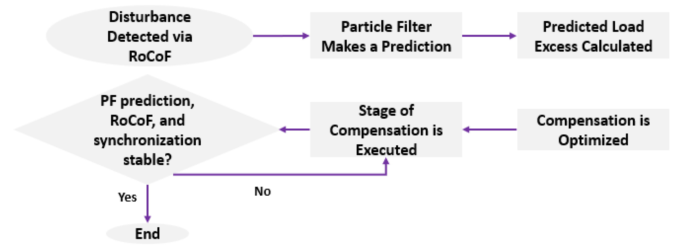
• Disturbances are detected using the rate of change of frequency (RoCoF).
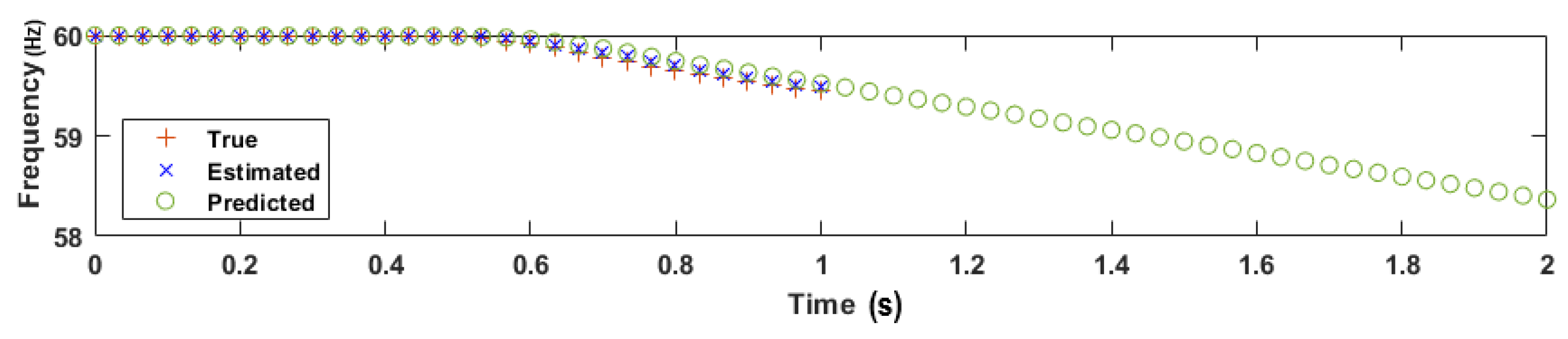
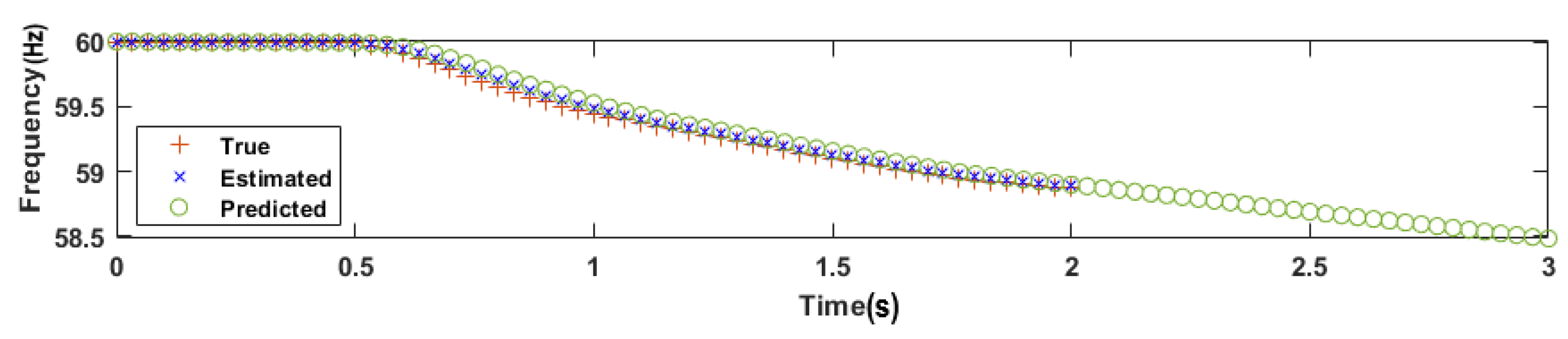
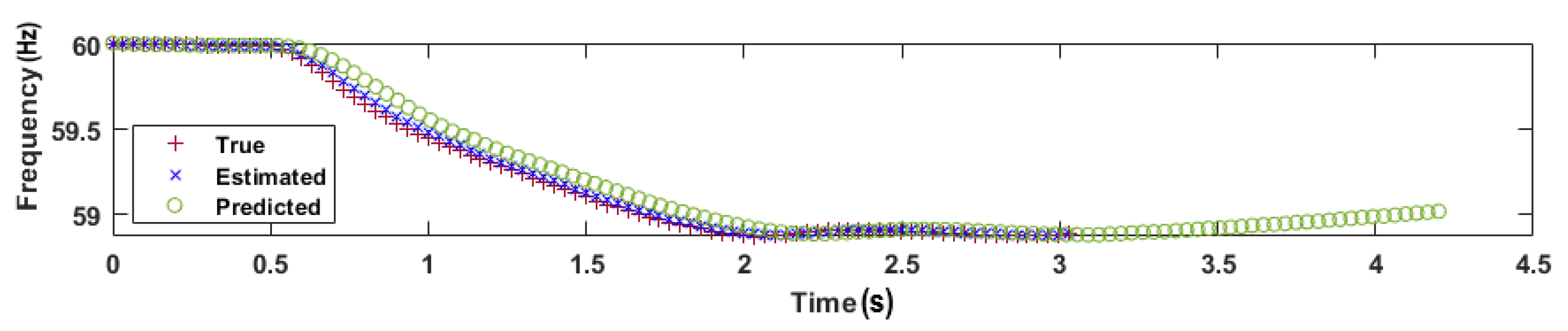
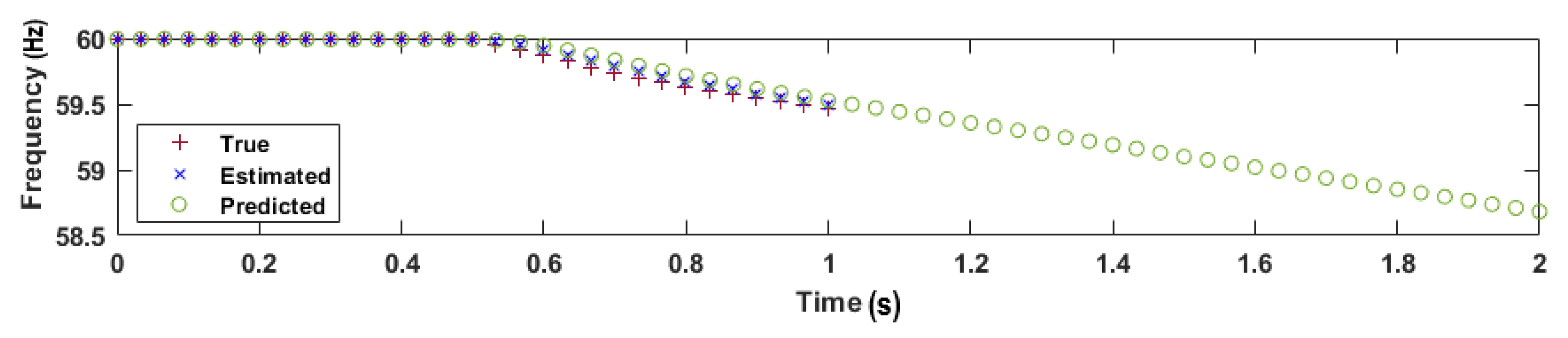
• The state of frequency is predicted one to three seconds into the future.
• A load excess factor is determined using the predicted state of frequency.
• Using loading data collected at the feeder level, the method finds a suitable combination of load (feeders) that will be dropped in stages to meet the excess load factor and regain load-generation balance.

This paper is organized as follows: Section 2 provides a brief overview of the state-of-the-art. Basic theory is presented in Section 3. An overview of the proposed solution including an illustrative example are given in Section 4. Comparative case studies are found in Section 5. Finally, concluding remarks are given in Section 6.

2. State-of-the-Art

A solution that predicts the state of frequency after a disturbance is presented in [6]. This method derives an approximate model from PMU readings and when a disturbance is detected it predicts a new steady state operating point. Using the predicted frequency value, the amount of load to be shed is calculated. One of the highlights of this technique is that very few assumptions are made in the context of inertia and generator governors. However, the performance of [6] is highly dependent on system observability. Also, convergence times are highly variable, and in some cases it takes up to two seconds for the algorithm to provide a load excess factor. The uncertainty produced by variable processing times is an important limitation. For this reason, this solution is suited for systems with high inertia where processing time requirements are not as stringent.

In [7], curves are projected a few seconds into the future to estimate the future state of frequency. Polynomial curve fitting is used to produce these predictions. One of the main appeals of this technique is its simplicity; however, the technique has several limitations. First, high PMU sampling rates are used. This is a critical parameter that determines the feasibility of the technique, as higher sampling rates place a significant burden on communication systems [8]. Second, in [7] the algorithm alternates between first and second degree polynomials based on assumptions. Finally, the authors assume that deviations will follow a mostly linear pattern. These assumptions limit the type of systems where this technique can be implemented.

In [9], frequency is monitored continuously through a feedback controller. Load excess calculations are updated in real time reducing overshedding. A customized version of a PMU is developed in [10]. Measurements captured at fast sampling rates are used to detect and correct issues early. A multilevel load shedding solution is presented in [11]. This technique leverages neural networks to predict the trajectory of frequency after a disturbance. A similar technique based on deep Q learning, developed for micro-grids, is presented in [12]. An index based approach is introduced in [13]. Historical data is used to calculate a capacity index which is then used for load shedding. Performance issues in micro-grid UFLS related to lack of communication and dynamic inertia are addressed in [14]. The proposed technique analyzes the droop characteristics of the system and makes decisions when values deviate from the reference. A frequency stability control method based on topology control is presented in [15]. The goal of this method is to prevent load shedding by switching transmission lines.

Power measurements and power injections have also been proposed as a means of monitoring and controlling power system stability. In [16], DERs are actuated to compensate generation-load imbalances. The method uses the extended Kalman filter to drive DERs in real-time. A frequency stability solution based on monitoring the active power injections from synchronous condensers (SCs) is presented in [17]. A novel aspect of this method is that it offers an alternative to RoCoF detection. The premise of this method is that valuable information such as the loss of a generating unit can be retrieved from the change in the active power injection from an SC. It is suggested that disturbances can be detected earlier by monitoring power injections from SCs compared to RoCoF based methods. In [18], a predictive transient stability mitigation method is presented. After a disturbance occurs, the center of oscillations (CoO) produced by the disturbance is located. This is done by comparing the frequencies at the two ends of the line. Once the location of the CoO has been identified, a simplified equivalent model is created. By monitoring the potential and the total energy (the sum of potential and kinetic energies) of the system, the affected generator can be seen drifting into instability before any thresholds are surpassed. A similar set of ideas is applied in [19] to develop an UFLS scheme based on RoCoF and the center of inertia (CoI). Inflections in the projection of the estimated CoI with respect to the RoCoF are used to detect disturbances.

3. Background

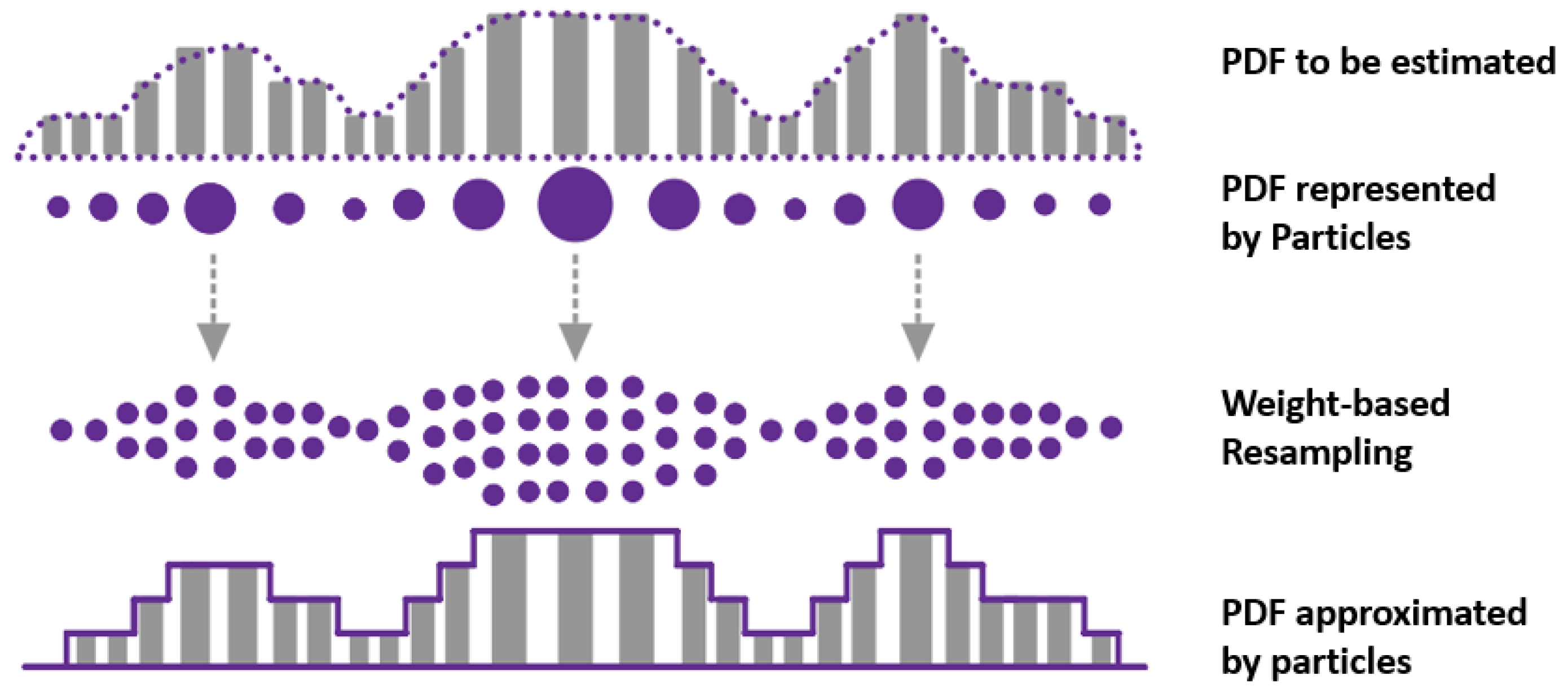
3.1. Particle Filter

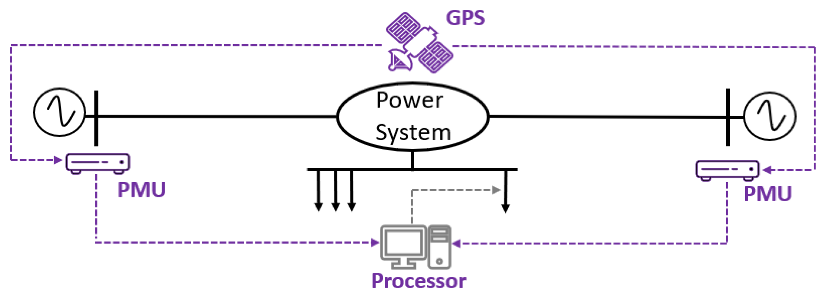
The particle filter (PF), is a type of Bayesian filter that estimates probability distributions via particles. The PF combines data from statistical models with data produced by an underlying system model [20]. At each time step, predictions and corrections are made similar to the Kalman filtering process [21]. The PF is not limited to Gaussian distributions and has an inherent ability to quantify uncertainty [22,23,24,25].

Mathematically, the PF combines elements from the Monte Carlo method and Bayesian estimation. The estimated state along with uncertainties are calculated from probability density functions (PDFs) [26]. Being a Bayesian filter, the PF updates its prior and posterior at each time step. Given a process model, the prior can be updated using the following equation:

$$p\left(x_k\right|z_{1:k-1})=\int p\left(x_k\right|x_{k-1})p\left(x_{k-1}\right|z_{1:k-1})d{x}_{x-1}$$

(1)

Here, p is the posterior obtained from a PDF with inputs $u_{1:k}$, and measurements $z_{1:k}$. Inputs $u_k$, and the previous state $x_{x-1}$ are used to provide an updated state x, at time step k. This prior is a guess based on information received up to time step $k-1$. With this prior, Bayes’ theorem can be utilized to obtain the new posterior.

The steps described so far are very similar to the steps involved in Kalman filtering. A key feature that differentiates the PF from the KF, is the PF’s use of the Monte Carlo method. When searching for an optimal Bayesian solution, the PF evaluates a sum of weighted samples, known as particles:

$$p\left(x_{0:k}\right|z_{1:k})\approx {\Sigma }_{i=1}^{N_s}{w}_k^i\delta (x_{0:k}-x_{0:k}^i)$$

(2)

In Equation (2), $N_s$ represents the number of samples in a set. $\delta (·)$ refers to the Dirac delta function. $w_k^i$ represents the weight of each particle $x_{0:k}^i$.

Subsequent mathematical manipulations of Equation (2) yield Equation (3):

$$p\left(x_k\right|z_{1:k})\approx {\Sigma }_{i=1}^{N_s}{w}_k^i\delta (x_k-x_k^i)$$

(3)

An important principle of the PF can be observed through (3), which is that the solution approaches the real values as the number of particles is increased [26].

Another pivotal element of the PF process is the concept of resampling. Resampling in the PF is analogous to the correction step in the KF. The PF resamples with the goal of correcting imbalances in particle weights [20]. The estimation process conducted by the PF is illustrated by Figure 1.

The system model used in this work is a simple sinusoidal. This underlying model was chosen because it is consistent with the oscillatory behavior of power system frequency. For the interested reader, an in-depth look at the theory behind the PF and its mathematical formulation are provided in [26]. Furthermore, multiple variations of Bayesian filters, including the PF are compared in [27].

3.2. Synchrophasors

Synchrophasors are electrical measurements sharing a common reference. These measurements are commonly synchronized via GPS clocks. Figure 2 offers a basic depiction of the framework.

Devices that support synchrophasors are referred to as phasor measurement units or PMUs. PMUs have relatively high sampling rates, in some cases up to 120 frames per second (fps) [28]. These sampling rates combined with the synchronization of measurements, make it possible to derive input-output pairs that can be used to build mathematical models [29].

One common assumption made by PMU-based solutions is that high PMU sampling rates will be viable. Sampling rate limitations are in part driven by the capacity of communication networks. High PMU sampling rates could overwhelm communication networks in terms of data transfer and data storage [8,29]. With these limitations in mind, 30 fps seems to offer a balance between practicality and estimation accuracy. Estimation across multiple sampling rates is performed in [30], with 30 fps delivering an acceptable performance relative to higher sampling rates.

3.3. Disturbance Detection

Techniques that utilize derivatives or rate of change, to detect frequency disturbances are referred to as semi-adaptive techniques [31]. Semi-adaptive techniques offer a good balance between security and dependability [32]. In this work, the rate of change of frequency (RoCoF), represented by R, is used as the primary means of disturbance detection. R can be computed as:

$$R=\frac{f_2-f_1}{dt}$$

(4)

In Equation (4), $f_1$ refers to the frequency at the start of the measurement period, and $f_2$ is frequency at the end of the period. $dt$ represents the duration of the period in seconds. One of the benefits of semi-adaptive detection is that it allows for intentional delays to be part of the scheme. These delays give the system a brief opportunity to self-correct issues before corrective actions are taken. The duration of these delays is inversely proportional to R. In this work, the thresholds and their respective delays were taken from [33].

3.4. Prediction

This work introduces a simple, yet effective way to predict the future state of frequency using the particle filter. By default the PF will make predictions; however, these predictions extend only $k+1$ time steps into the future [26]. The time horizon of these predictions can be extended without significant modifications to the PF algorithm if measurements are augmented with artificial data points. The idea here is to use measurements to derive artificial data points, which are then processed by the PF. The output of the PF are estimates based on historical data, the underlying system model, and artificial data. From the perspective of the user, since these estimates are in the future, they can be considered a prediction. The artificial data points (ADPs) are computed as follows:

$$\begin{array}{cc}\hfill AD{P}_i& \hfill =AD{P}_{i-1}+t_s{f}^{\prime }+t_s^2{f}^{″}\hfill \end{array}$$

(5)

where $AD{P}_{i-1}$, is the previous ADP, or the last measurement when $i=1$. $f^{\prime }$ and $f^{″}$ are the first and second frequency derivatives, respectively. $t_s$ represents the time window of the derivatives. These derivatives play a key role in determining the degree of influence system dynamics have on the ADPs. Derivatives calculated using only a few measurements produce a set of ADPs that is very dynamic (sensitive to changes), which can be useful in some situations, this is explored in the case studies. The number of measurements used in the derivation of the ADPs can be adjusted to increase (or decrease) the sensitivity of the algorithm to system dynamics as desired. This is similar to the tuning of Q and R parameters in the KF. These parameters are tuned to find a balance between new and historical data [34]. A compromise was found by averaging the change of the last ten measurements and then dividing this value by $t_s$. One can think of this as an average derivative. ADP computation is a sequential process that starts with the last measurement received. The derivatives are then used to adjust the previous ADP to produce the next one. The result is a vector containing the ADPs that will be the basis of predictions.

The time horizon of the prediction can be adjusted based on the number of ADPs used. For a desired time horizon, $t_p$, the desired number of ADPs can be found per:

$$N_{ADP}=t_p{f}_s$$

(6)

The number of ADPs, $N_{ADP}$, is a function of the sampling rate $f_s$, and the time horizon of the prediction, $t_p$, which is measured in seconds. The process of ADP generation is summarized as follows, see Algorithm 1:

Algorithm 1 ADP Generation

Initialization:   $AD{P}_{i-1}$ = Last measurement   $f^{\prime }$ = Average first derivative in last 10 measurements   $f^{″}$ = Average second derivative in last 10 measurements   $N_{ADP}$ = Number of ADPs required 1:  for $i=1$ to $N_{ADP}$ do 2:   $AD{P}_i=AD{P}_{i-1}+t_s{f}^{\prime }$    $f^{\prime }=f^{\prime }+t_s{f}^{″}$ 3:  end for

In this work, after an initial prediction is made, subsequent predictions are made with an emphasis on new data. Before a subsequent load shedding stage is executed, synchronization between the machines is considered. Surprisingly, synchronization is often overlooked in frequency stability solutions in literature [29]. In this work, machine rotor angles are assumed to be tracked via relays at the same sampling rate used for frequency. The difference between the rotor angles, $\Delta \theta$, together with the predicted state of frequency are used to determine the need for additional load shedding stages. This aspect of the solution will explored in the case studies presented on Section 5.

3.5. Excess Loading Equations

After a prediction indicating the need for corrective actions is made, predicted frequency values are used to calculate the corresponding load excess L. The load excess can be calculated via the following expression, which is itself derived from the swing equation [35]:

$$L=\frac{RH(1-\frac{f_2^2}{f_1^2})}{p(f_2-f1)}$$

(7)

Here, parameter f refers to frequency measurements. $f_1$ is the frequency at the beginning, while $f_2$ is the frequency at the end of the measurement period. R is the RoCoF found via Equation (4). p is the power factor, while the inertia coefficient is represented by H. When L is calculated using predicted values, a modified version of Equation (7) is used to calculate the corresponding predicted load excess $L_p$:

$$L_p=\frac{R_p{H}_{est}(1-\frac{f_p^2}{f_1^2})}{p(f_p-f_1)}$$

(8)

In Equation (8), $f_p$ is the predicted frequency. $R_p$ is still the RoCoF, but now this parameter is calculated as the change from $f_1$, to the predicted frequency $f_p$, over the prediction period. Power factor p is calculated the same before, meanwhile $H_{est}$, is now an estimated coefficient of inertia. The process of obtaining $H_{est}$ is described on the next section.

3.6. Online H Estimation

The sampling rates and synchronization of PMUs make it possible to utilize system identification algorithms to estimate power system parameters [29]. One such approach, subspace estimation, has delivered encouraging results in power systems applications [36,37,38]. This work adopts an H estimation approach presented in [39], where H is estimated online from frequency and power measurements. As presented in [39], the online H estimation algorithm is not compatible with the framework developed in this paper. The original formulation utilizes high PMU sampling rates (100 fps), and the necessary data is collected over long time windows. Therefore, two simple modifications are made:

• The sampling rate is decreased to 30 fps, a much more manageable data transfer rate [8,40].
• Estimation of H is carried out periodically as opposed to in real-time. Historical data and forecasts can be used to reduce the number of times H is estimated. This work uses dynamic loading (modeled from real life data available at [41]), and the procedure is run the equivalent of six times per day. For the case studies presented on Section 5, H is assumed to have been estimated roughly two hours before the events take place.

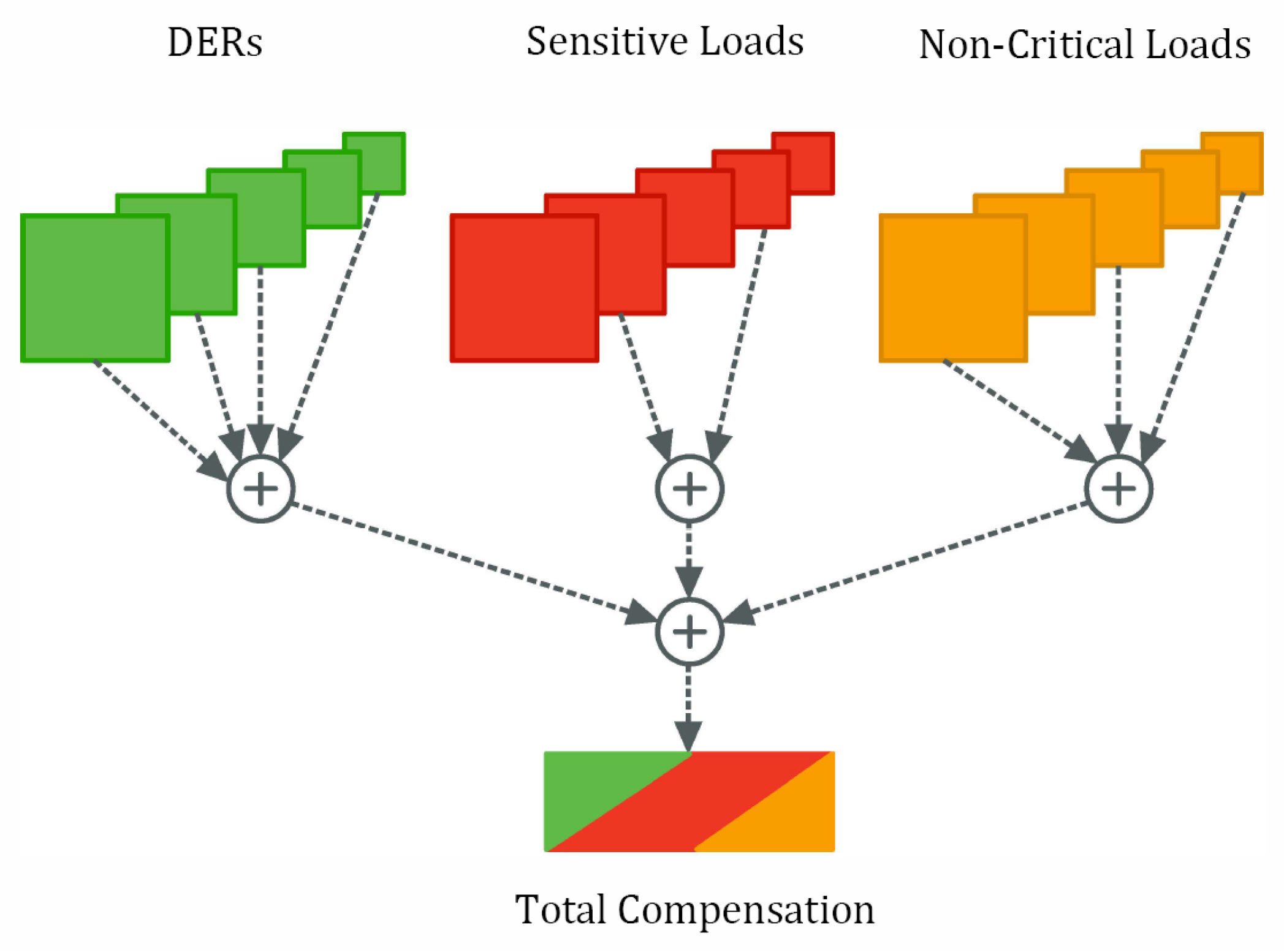
3.7. Optimizing the Response

Mixed integer linear programming (MILP) is used to optimize the response. An objective function is minimized subject to a set of constraints. The algorithm iterates until it finds an optimal solution. The iteration process can be carried out in different ways depending on the requirements defined by the user. MILP offers advantages in terms of ease of implementation due to its relatively low complexity, and its ability to incorporate relaxations [42]. In terms of cost, in this work, DERs are given the lowest penalty among the three sources of compensation. This is followed by non-critical loads (i.e., residential loads). Sensitive loads carry the highest cost as these represent industrial operations where an outage can lead to significant losses in revenue or equipment damage. Critical or life-safety loads were not considered in this work as these loads are usually not dropped intentionally [35]. A general MILP problem can be formulated as [43]:

$$\begin{array}{c}\hfill \mathrm{Minimize}J=c^{T}x+d^{T}y\end{array}$$

(9a)

$$\begin{array}{c}\hfill \mathrm{s}.\mathrm{t}.Ax+By\ge b\end{array}$$

(9b)

$$\begin{array}{ccc}\hfill (x,y)\in {\mathbb{R}}^n\times {\mathbb{Z}}^p{x}_j\in \mathbb{R}& \hfill \hfill & \hfill \mathrm{for}j\in \mathcal{C}\end{array}$$

(9c)

where A is an $m\times n$ matrix, B is an $m\times p$ matrix, b is an m-dimensional vector, c is an n-dimensional vector, and d is an p-dimensional vector. c and d define the cost associated with selecting an agent from A and B, respectively. In this context, the term agent refers to sources of load excess compensation (i.e., load shedding or distributed energy resource (DER) actuation). These ideas are illustrated by Figure 3.

When deciding which agents to use, in addition to cost, the algorithm also considers factors such as distance from the disturbance, and the number of customers affected. For instance, it might be more desirable to drop one large industrial load instead of a large number of residential customers. Additional parameters can be added as required, and all parameters can be modified to meet a desired operational standard.

The information fed to the algorithm (capacity and loading information), is already collected at the substation level and transmitted to control centers [44]. This step would not place a significant burden on communication networks since all it requires is a periodical loading and capacity update. The process of optimizing the response can be summarized as follows, see Algorithm 2:

Algorithm 2 Load Balance Optimization

Initialization:   A = DER capacity available   B = Sensitive loads available to be shed (feeder level)   C = Non-critical loads available to be shed (feeder level)   $c_1^T$ = Cost of DER actuation   $c_2^T$ = Cost of shedding sensitive loads   $c_3^T$ = Cost of shedding non-critical loads   b = Calculated load excess 1:  Minimize J = $c_1^{t}x+c_2^{t}y+c_3^{t}z$    s.t. $Ax+By+Cz\ge b$ 2:  Return Selected agents in A, B, and C

As previously stated, the optimization routine can be easily modified to include additional agent types, costs, or constraints. After the optimal combination of DERs and loads for compensation has been identified, a trip signal is sent to the selected feeder breakers.

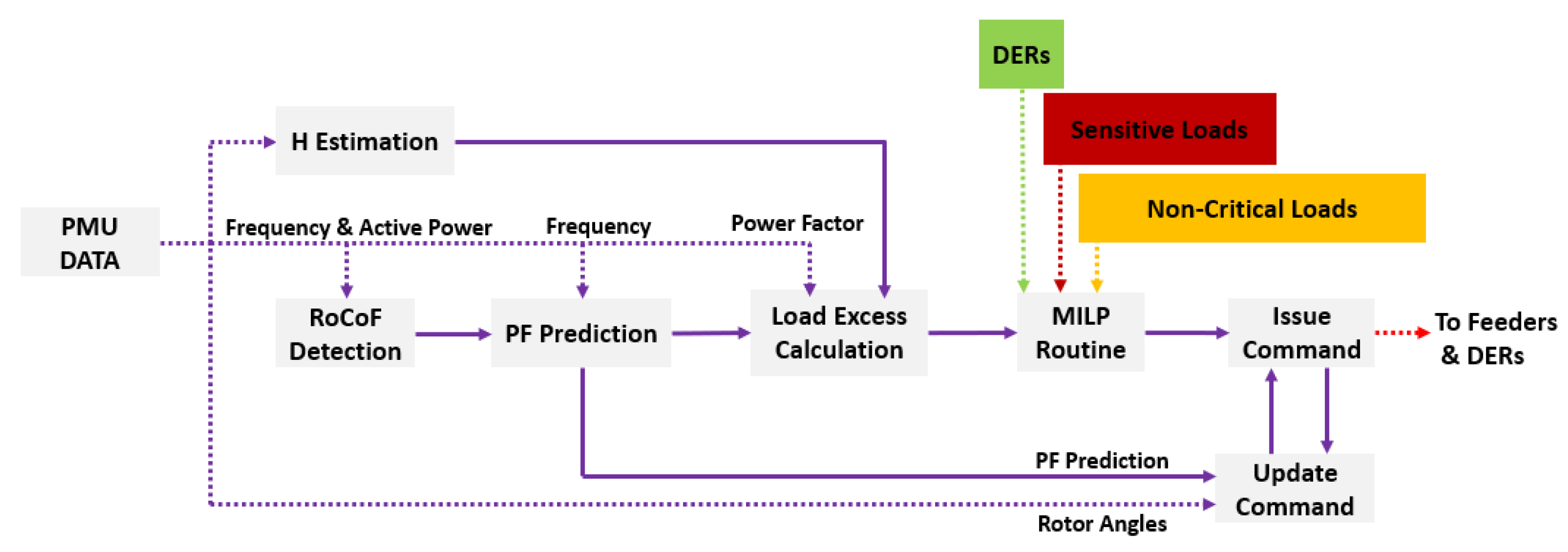
4. Overview in Distributed Form

This method is intended to operate as a distributed solution overseeing the frequency stability of an area of the grid. PMUs at the edge of an area share information with selected PMUs at neighboring areas, as depicted in Figure 4. In this work, each area is previously defined. Figure 4 illustrates a distributed framework with 4 areas, considering the IEEE 14-Bus system [45].

Figure 5 shows the modules that make up this proposed solution.

Related techniques in literature assume a processing time of roughly 500 ms. This includes 400 ms due to communication delays, and 100 ms that account for relay processing times and breakers operating times [6,7]. In this work a conservative delay of one full second is used.

Many of the operating parameters of this scheme are customizable, facilitating compliance with industry standards such as NERC PRC-006 [2]. Some of the ways this framework follows PRC-006 guidance include among others:

• Adjustable frequency thresholds.
• Adjustable number of load-shedding stages.
• Customizable islands (based on PMU availability).
• Additional parameters such as voltage levels, frequency overshoot, rotor angles, breaker status, and loading of power lines can be integrated as constraints as long as the networks can support it.
• This method eliminates the need for simulations to establish underfrequency load-shedding (UFLS) contingencies.

A flow diagram of the process is depicted by Figure 6.

5. Case Studies

This section contains three case studies that showcase the advantages of the presented method under different operating conditions and constraints. Each case study includes key performance metrics as well as comparisons with other methods found in literature. Before proceeding to the test cases, an illustrative example is presented. The purpose of the example is to summarize the topics and steps discussed in the previous sections.

5.1. Illustrative Example

Figure 7 illustrates the complete response of a four-machine system after a disturbance is introduced and mitigated using the scheme presented in this work.

The disturbance starts at 0.5 s, and it is detected via the RoCoF from Equation (4). At 1 s, a prediction is made as shown in Figure 8. Dotted vertical lines in red, considering Figure 7, represent compensation stages derived with the solution. To account for processing and communication delays, corrective actions are taken one full second after a prediction is made.

The method estimates the state of the system frequency one second into the future. These estimates are then used to calculate the loading excess via Equation (8), which is then followed by a compensation stage at 2 s, as seen in Figure 7. A second prediction is made immediately after the first stage of compensation, this is shown in Figure 9.

Based on this new prediction, a second stage of compensation is executed at 3 s, which is then followed by a third prediction as illustrated in Figure 10.

The third prediction shows that the frequency is trending back into stability. Since frequency is expected to return to its normal range, a third stage of compensation is not executed. In this case the system regains stability with minimal overshoot as seen in Figure 11.

Subsequent stages of compensation are not executed when three conditions are met:

• The PF predicts a rise in frequency.
• The RoCoF is positive.
• Machine synchronization is stable.

The goal of the method is to first stop the decay in frequency, and second, to send it back to a range where generator governors can stabilize it.

5.2. Case Study I

This case study contains four scenarios and it is based on Kundur’s Two-Area System. This model can be found at [46]. The locations where excesses in load are introduced are numbered (1 through 4) in Figure 12. Loading, capacity, and other operational parameters are presented in

Table 1. Load flow data.

Bus	V (pu)	${\mathit{P}}_{\mathit{G}}$ (MW)	${\mathit{P}}_{\mathit{L}}$ (MW)	${\mathit{Q}}_{\mathit{L}}$ (MVar)	${\mathit{Q}}_{\mathit{C}}$ (MW)
1	1.03	615	-	-	-
2	1.01	700	-	-	-
3	1.03	719	-	-	-
4	1.01	700	-	-	-
7	-	-	967	100	200
9	-	-	1767	100	350

and

Table 2. Generator dynamic data.

Generator	Rating	${\mathit{X}}_{\mathit{d}}$	${\mathit{X}}_{\mathit{d}}^{\prime }$	${\mathit{X}}_{\mathit{d}}^{″}$	${\mathit{T}}_{\mathit{d}0}^{\prime }$	${\mathit{T}}_{\mathit{d}0}^{″}$	${\mathit{X}}_{\mathit{q}}^{\prime }$	${\mathit{X}}_{\mathit{q}}^{″}$	${\mathit{T}}_{\mathit{q}0}^{\prime }$	${\mathit{T}}_{\mathit{q}0}^{″}$	H
	(MVA)	(pu)	(pu)	(pu)	(s)	(s)	(pu)	(pu)	(s)	(s)	(s)
G1	900	1.8	0.3	0.25	8	0.03	1.7	0.25	0.4	0.05	6.5
G2	900	1.8	0.3	0.25	8	0.03	1.7	0.25	0.4	0.05	6.5
G3	900	1.8	0.3	0.25	8	0.03	1.7	0.25	0.4	0.05	6.175
G4	900	1.8	0.3	0.25	8	0.03	1.7	0.25	0.4	0.05	6.175

, and also in

Table A1. System loading and capacity for Case Study I.

Disturbance Location	Total DER Capacity	Excess Loading
1	5%	18%
2	3%	21%
3	6%	20%
4	8%	22%

in the Appendix A. Considering Figure 12, buses are referred by numbers, loads by the letter ‘L’ followed by a number, capacitor banks by the letter ‘C’ followed by a number, and generators by the letter ‘G’ followed by a number. Again, to account for processing and communication delays, corrective actions are taken one full second after a prediction is made. Gaussian noise with a variance of 0.025 is added to the measurements.

The scenario where the load excess is placed at bus 1 in Figure 12, is run twice. First, a fixed three stage compensation procedure is used. The first compensation stage is set at 50% of the calculated load excess. Stages 2 and 3 compensate 25% of the load excess each, for a total of 100%, similar to the approach used by [7]. The load imbalance starts at 0.5 s, and each compensation stage is illustrated through vertical dotted red lines in Figure 13.

In this case the system was successful in first, arresting the decline in frequency, and second, in providing a smooth transition back to steady state. Three predictions were made by the particle filter, they are presented in Figure 14, Figure 15 and Figure 16:

This same scenario was performed using a version of the algorithm referred to as adaptive compensation. Adaptive compensation works as follows: The initial stage compensates for 50% of the estimated excess load factor. After the first stage is executed, the number of samples used in obtaining the derivatives in Equation (5) is decreased, making the particle filter more receptive to system dynamics. Compensation with variable stages is illustrated in Figure 17 through a red dotted vertical line.

In this case, the PF predicts that frequency will be returning to levels close to the reference after only one stage of compensation. This is shown in Figure 18.

With frequency expected to return to its normal range, and $\Delta \theta$ not trending towards loss of synchronism, further compensation stages are avoided. Being able to restore frequency stability while compensating only a portion of the calculated load excess happens for two reasons: First, being able to take corrective actions early means that compensation can begin before the system reaches a critical state. Second, generator governors and other controllers are not considered during compensation calculations, and while this might lead to some inaccuracies, it also gives the scheme a safety margin, which translates into a lower amount of load shed. Realistically, a highly accurate load compensation value is difficult to obtain given the time constraints and the dynamics of both the loads and the sources. Moreover, it has been suggested that in the context of frequency stability, early action trumps accuracy [7].

This scenario is performed once again with the adaptive compensation procedure, but this time, polynomial curve fitting (PCF) as presented in [7], is used to obtain predictions instead of the PF. After the first stage of compensation has been executed, a follow up prediction is made as illustrated by Figure 19.

The prediction obtained via polynomial curve fitting is unable to leverage the dynamics of the system the way the PF can, leading to further stages of compensation.

Three more disturbances are introduced and both the PF based method and the PCF technique are used to mitigate them. A performance comparison is presented in

Table 3. Key metrics for Case Study I.

Disturbance Location	Method	Number of Stages	% of Load Excess Compensated
1	PF	1	50%
	PCF	3	100%
2	PF	2	75%
	PCF	3	100%
3	PF	2	75%
	PCF	3	100%
4	PF	1	50%
	PCF	3	100%

.

For the four scenarios presented in Table 3, the method presented in this paper was able to bring the system back into stability while shedding $25\%$ to $50\%$ less load. This is, as previously discussed, due to the ability of the prediction model to leverage the dynamics of the system as frequency begins to return to a stable condition. Performance metrics are examined in

Table 4. Overshoot values for Case Study I.

Disturbance Location	Number of Stages	Overshoot
1	1	−0.83%
2	2	1.13%
3	2	0.91%
4	1	2.1%

, where frequency overshoot during recovery is measured.

As expected, more stages lead to a smoother transition back into steady state. It is worth noting that even when only one compensation stage was used, the overshoot was still fairly low.

5.3. Case Study II

A second case study was conducted using the IEEE 14-Bus System as reference. Following the same process as in the first case study, four scenarios are presented. The locations where the load excesses are introduced are presented in Figure 20, through numbers. Loading, capacity, and other operational parameters are presented in

Table A2. System loading and capacity for Case Study II.

Disturbance Location	Machine	Loading %	Total DER Capacity	Excess Loading
1	1	80%	5%	17%
	2	85%
	3	88%
	4	90%
	5	85%
2	1	80%	4%	21%
	2	90%
	3	85%
	4	85%
	5	80%
3	1	90%	5%	19%
	2	88%
	3	80%
	4	80%
	5	85%
4	1	85%	2%	20%
	2	85%
	3	85%
	4	85%
	5	85%

in the Appendix A.

Once again, each scenario is run twice, one time using PCF to build a base line and then using the PF. Key metrics are presented in

Table 5. Key metrics for Case Study II.

Disturbance Location	Method	Number of Stages	% of Load Excess Compensated
1	PF	1	50%
	PCF	3	100%
2	PF	2	75%
	PCF	3	100%
3	PF	1	50%
	PCF	3	100%
4	PF	1	50%
	PCF	3	100%

.

The results of this case study are consistent with the results of the first one, and they show that the PF based method facilitates the recovery of frequency while greatly reducing the amount of compensation used. Overshoot is also used as a performance metric for this case study, and the results are presented in

Table 6. Overshoot values for Case Study II.

Disturbance Location	Number of Stages	Overshoot
1	1	2.3%
2	2	0.84%
3	1	−1.72%
4	1	1.93%

.

The observed overshoot in this scenario is once again fairly low, which is consistent with the results obtained in the first case study.

5.4. Case Study III

The goal of this final test case is to highlight the flexibility of the method and use it to drive distributed energy resources (DERs) in real-time. This test was run under a similar set of assumptions as those made in [16], where a KF-based compensation method is presented. In order to test the algorithm under demanding conditions, faster frequency deviations than those seen in [16] were generated. Most importantly, the total delay time involved in the processing of data and actuation of DERs was increased to 500 ms; up from the 40 ms time delay used in [16]. That is a response time over ten times slower.

Frequency deviations start at 1 s, with a significant loss of generation at 1.5 s. As illustrated in Figure 21, DER actuation takes place 0.5 s after the frequency deviations.

As before, measurements are made via PMUs at 30 fps. The power mismatch is calculated continuously in this test case per Equations (4) and (8) in the form of a controller. As shown in Figure 21 above, the frequency and power mismatch follow virtually the same trend but in opposite directions. When frequency deviates from the 60 Hz reference, a corresponding current output is seen from the DERs. The compensation is based on the power mismatch calculated by the controller. Despite having a 0.5 s delay, the system successfully mitigates the frequency deviations.

6. Conclusions

This work presented a distributed scheme for proactive frequency stability. By being able to estimate the future state of frequency, corrective actions can be taken before the system reaches a critical condition. This proactive approach makes it possible to optimize the response to a disturbance thereby reducing the amount of compensation utilized. The method was tested via simulations based on Kundur’s Two-Area System, and the IEEE 14-Bus System. The results were promising and outperformed other contemporary solutions by drastically reducing the amount of load dropped during compensation. Future work will focus on streamlining the solution by reducing requirements in terms of data and the number of PMUs utilized. Alternative optimization methods as well as improving the robustness of the particle filter will also be investigated.

References

1. Sigrist, L.; Rouco, L.; Echavarren, F.M. A review of the state of the art of UFLS schemes for isolated power systems. Int. J. Electr. Power Energy Syst. 2018, 99, 525–539. [Google Scholar] [CrossRef]
2. NERC Standards PRC-006-SERC-02; NERC Standards PRC-006-SERC-02. NERC: New York, NY, USA, 2017. Available online: https://www.nerc.com/pa/Stand/Pages/PRC006SERC02RI.aspx (accessed on 14 February 2023).
3. IEEE Std. C37.117-2007; IEEE Guide for the Application of Protective Relays Used for Abnormal Frequency Load Shedding and Restoration. IEEE: New York, NY, USA, 2007; p. c1.
4. Rudez, U.; Mihalic, R. A novel approach to underfrequency load shedding. Electr. Power Syst. Res. 2011, 81, 636–643. [Google Scholar] [CrossRef]
5. Sigrist, L.; Egido, I.; Rouco, L. Principles of a Centralized UFLS Scheme for Small Isolated Power Systems. IEEE Trans. Power Syst. 2013, 28, 1779–1786. [Google Scholar] [CrossRef]
6. Larsson, M.; Rehtanz, C. Predictive frequency stability control based on wide-area phasor measurements. IEEE Power Eng. Soc. Summer Meet. 2005, 1, 233–238. [Google Scholar] [CrossRef]
7. Rudez, U.; Mihalic, R. WAMS-Based Underfrequency Load Shedding with Short-Term Frequency Prediction. IEEE Trans. Power Deliv. 2016, 31, 1912–1920. [Google Scholar] [CrossRef]
8. Bose, A. Smart Transmission Grid Applications and Their Supporting Infrastructure. IEEE Trans. Smart Grid 2010, 1, 11–19. [Google Scholar] [CrossRef]
9. Li, C.; Wu, Y.; Sun, Y.; Zhang, H.; Liu, Y.; Liu, Y.; Terzija, V. Continuous Under-Frequency Load Shedding Scheme for Power System Adaptive Frequency Control. IEEE Trans. Power Syst. 2020, 35, 950–961. [Google Scholar] [CrossRef]
10. Yao, W.; You, S.; Wang, W.; Deng, X.; Li, Y.; Zhan, L.; Liu, Y. A Fast Load Control System Based on Mobile Distribution-Level Phasor Measurement Unit. IEEE Trans. Smart Grid 2020, 11, 895–904. [Google Scholar] [CrossRef]
11. Li, Q.; Xu, Y.; Ren, C. A Hierarchical Data-Driven Method for Event-Based Load Shedding Against Fault-Induced Delayed Voltage Recovery in Power Systems. IEEE Trans. Ind. Inform. 2021, 17, 699–709. [Google Scholar] [CrossRef]
12. Wang, C.; Yu, H.; Chai, L.; Liu, H.; Zhu, B. Emergency Load Shedding Strategy for Microgrids Based on Dueling Deep Q-Learning. IEEE Access 2021, 9, 19707–19715. [Google Scholar] [CrossRef]
13. Hussain, A.; Bui, V.-H.; Kim, H.-M. An Effort-Based Reward Approach for Allocating Load Shedding Amount in Networked Microgrids Using Multiagent System. IEEE Trans. Ind. Inform. 2020, 16, 2268–2279. [Google Scholar] [CrossRef]
14. Dehghanpour, E.; Karegar, H.K.; Kheirollahi, R. Under Frequency Load Shedding in Inverter Based Microgrids by Using Droop Characteristic. IEEE Trans. Power Deliv. 2021, 36, 1097–1106. [Google Scholar] [CrossRef]
15. Brown, W.E.; Moreno-Centeno, E. Transmission-Line Switching for Load Shed Prevention via an Accelerated Linear Programming Approximation of AC Power Flows. IEEE Trans. Power Syst. 2020, 35, 2575–2585. [Google Scholar] [CrossRef]
16. Pulendran, S.; Tate, J.E. Energy Storage System Control for Prevention of Transient Under-Frequency Load Shedding. IEEE Trans. Smart Grid 2017, 8, 927–936. [Google Scholar] [CrossRef]
17. Sauhats, A.; Utans, A.; Silinevics, J.; Junghans, G.; Guzs, D. Enhancing Power System Frequency with a Novel Load Shedding Method Including Monitoring of Synchronous Condensers’ Power Injections. Energies 2021, 14, 1490. [Google Scholar] [CrossRef]
18. Farantatos, E.; Huang, R.; Cokkinides, G.J.; Meliopoulos, A.P. A Predictive Generator Out-of-Step Protection and Transient Stability Monitoring Scheme Enabled by a Distributed Dynamic State Estimator. IEEE Trans. Power Deliv. 2016, 31, 1826–1835. [Google Scholar] [CrossRef]
19. Sun, M.; Liu, G.; Popov, M.; Terzija, V.; Azizi, S. Underfrequency Load Shedding Using Locally Estimated RoCoF of the Center of Inertia. IEEE Trans. Power Syst. 2021, 36, 4212–4222. [Google Scholar] [CrossRef]
20. Xu, Y.; Xu, K.; Wan, J.; Xiong, Z.; Li, Y. Research on Particle Filter Tracking Method Based on Kalman Filter. In Proceedings of the IEEE Advanced Information Management, Communicates, Electronic and Automation Control Conference (IMCEC), Xi’an, China, 25–27 May 2018; pp. 1564–1568. [Google Scholar] [CrossRef]
21. Li, T.; Sattar, T.P.; Sun, S. Deterministic resampling: Unbiased sampling to avoid sample impoverishment in particle filters. Signal Process. 2012, 92, 1637–1645. [Google Scholar] [CrossRef]
22. Wang, S.; Zhao, J.; Huang, Z.; Diao, R. Assessing Gaussian Assumption of PMU Measurement Error Using Field Data. IEEE Trans. Power Deliv. 2018, 33, 3233–3236. [Google Scholar] [CrossRef]
23. Yang, T.; Mehta, P.G.; Meyn, S.P. Feedback particle filter with mean-field coupling. In Proceedings of the 2011 50th IEEE Conference on Decision and Control and European Control Conference, Orlando, FL, USA, 12–15 December 2011; pp. 7909–7916. [Google Scholar] [CrossRef]
24. Yang, T.; Laugesen, R.S.; Mehta, P.G.; Meyn, S.P. Multivariable feedback particle filter. Automatica 2016, 10–23. [Google Scholar] [CrossRef] [Green Version]
25. Yang, T.; Mehta, P.G.; Meyn, S.P. A mean-field control-oriented approach to particle filtering. In Proceedings of the 2011 American Control Conference, San Francisco, CA, USA, 29 June–1 July 2011; pp. 2037–2043. [Google Scholar] [CrossRef]
26. Elfring, J.; Torta, E.; van de Molengraft, R. Particle Filters: A Hands-On Tutorial. Sensors 2021, 21, 438. [Google Scholar] [CrossRef] [PubMed]
27. Arulampalam, M.S.; Maskell, S.; Gordo, N.; Clapp, T. A tutorial on particle filters for online nonlinear/non-Gaussian Bayesian tracking. IEEE Trans. Signal Process. 2002, 139, 174–188. [Google Scholar] [CrossRef] [Green Version]
28. IEEE Std C37.118.1-2011 (Revision of IEEE Std C37.118-2005); IEEE Standard for Synchrophasor Measurements for Power Systems. IEEE: New York, NY, USA, 2011; pp. 1–61. [CrossRef]
29. Paramo, G.; Bretas, A.; Meyn, S. Research Trends and Applications of PMUs. Energies 2022, 15, 5329. [Google Scholar] [CrossRef]
30. Paramo, G.; Bretas, A.; Meyn, S. High-Impedance Non-Linear Fault Detection via Eigenvalue Analysis with low PMU Sampling Rates. In Proceedings of the 2023 IEEE Power & Energy Society Innovative Smart Grid Technologies Conference (ISGT), Washington, DC, USA, 21–24 November 2023; pp. 1–5. [Google Scholar] [CrossRef]
31. Anderson, P.M.; Mirheydar, M. An adaptive method for setting underfrequency load shedding relays. IEEE Trans. Power Syst. 1992, 7, 647–655. [Google Scholar] [CrossRef]
32. Rudez, U.; Mihalic, R. Monitoring the First Frequency Derivative to Improve Adaptive Underfrequency Load-Shedding Schemes. IEEE Trans. Power Syst. 2011, 26, 839–846. [Google Scholar] [CrossRef]
33. SEL-751. Available online: https://selinc.com/products/751 (accessed on 1 July 2022).
34. Zhao, J.; Gómez-Expósito, A.; Netto, M.; Mili, L.; Abur, A.; Terzija, V.; Kamwa, I.; Pal, B.; Singh, A.K.; Qi, J.; et al. Power System Dynamic State Estimation: Motivations, Definitions, Methodologies, and Future Work. IEEE Trans. Power Syst. 2019, 34, 3188–3198. [Google Scholar] [CrossRef]
35. Horowitz, S.H.; Phadke, A.G. Power System Relaying, 4th ed.; Wiley: London, UK, 2014. [Google Scholar]
36. Paramo, G.; Bretas, A.S. WAMS Based Eigenvalue Space Model for High Impedance Fault Detection. Appl. Sci. 2021, 11, 12148. [Google Scholar] [CrossRef]
37. Nezam Sarmadi, S.A.; Venkatasubramanian, V.; Thomas, R.J. Electromechanical Mode Estimation Using Recursive Adaptive Stochastic Subspace Identification. IEEE Trans. Power Syst. 2014, 29, 349–358. [Google Scholar] [CrossRef]
38. Kim, J.; Tong, L.; Thomas, R.J. Subspace Methods for Data Attack on State Estimation: A Data Driven Approach. IEEE Trans. Signal Process. 2015, 63, 1102–1114. [Google Scholar] [CrossRef] [Green Version]
39. Zeng, F.; Zhang, J.; Chen, G.; Wu, Z.; Huang, S.; Liang, Y. Online Estimation of Power System Inertia Constant Under Normal Operating Conditions. IEEE Access 2020, 8, 101426–101436. [Google Scholar] [CrossRef]
40. Naduvathuparambil, B.; Valenti, M.C.; Feliachi, A. Communication delays in wide area measurement systems. In Proceedings of the Thirty-Fourth Southeastern Symposium on System Theory (Cat. No.02EX540), Huntsville, AL, USA, 19 March 2002; pp. 118–122. [Google Scholar] [CrossRef] [Green Version]
41. ERCOT. Grid Info: Load, Loading Data. 2022. Available online: http://www.ercot.com/gridinfo/load (accessed on 8 October 2022).
42. Carrion, M.; Arroyo, J.M. A computationally efficient mixed-integer linear formulation for the thermal unit commitment problem. IEEE Trans. Power Syst. 2006, 21, 1371–1378. [Google Scholar] [CrossRef]
43. Floudas, C.A.; Lin, X. Mixed Integer Linear Programming in Process Scheduling: Modeling, Algorithms, and Applications. Ann. Oper. Res. 2005, 139, 131–162. [Google Scholar] [CrossRef]
44. Schweitzer, E.O.; Whitehead, D.; Zweigle, G.; Ravikumar, K.G.; Rzepka, G. Synchrophasor-based power system protection and control applications. In Proceedings of the 2010 Modern Electric Power Systems, Wroclaw, Poland, 20–22 September 2010; pp. 1–10. [Google Scholar] [CrossRef]
45. Bretas, A.; Bretas, N.; London, J.; Carvalho, B. Cyber-Physical Power Systems State Estimation; Elsevier: Amsterdam, The Netherlands, 2021; Available online: https://www.sciencedirect.com/book/9780323900331/cyber-physical-power-systems-state-estimation (accessed on 1 November 2022).
46. Kundur, P. Simplified Synchronous Machine—Speed Regulation. MathWorks. Available online: https://www.mathworks.com/help/sps/ug/pmu-pll-based-positive-sequence-kundur-s-two-area-system.html;jsessionid=9f7bc00182f35350d6b467d0cb3c (accessed on 1 November 2022).
Figure 1. PDF estimation via particles.
Energies 16 04530 g001
Figure 2. Overview of the architecture.
Energies 16 04530 g002
Figure 3. Compensation agent selection via optimization.
Energies 16 04530 g003
Figure 4. Overview of the architecture in distributed form.
Energies 16 04530 g004
Figure 5. Overview of the algorithm and its modules.
Energies 16 04530 g005
Figure 6. Data flow diagram of the method.
Energies 16 04530 g006
Figure 7. Multi-stage compensation based on predictions.
Energies 16 04530 g007
Figure 8. First particle filter prediction.
Energies 16 04530 g008
Figure 9. Second particle filter prediction.
Energies 16 04530 g009
Figure 10. Third particle filter prediction.
Energies 16 04530 g010
Figure 11. Complete response estimated by the particle filter.
Energies 16 04530 g011
Figure 12. One line diagram of Case Study I.
Energies 16 04530 g012
Figure 13. Case Study I, scenario 1 results.
Energies 16 04530 g013
Figure 14. First prediction.
Energies 16 04530 g014
Figure 15. Second prediction.
Energies 16 04530 g015
Figure 16. Third prediction.
Energies 16 04530 g016
Figure 17. Scenario 1, PF compensation with adaptive stages.
Energies 16 04530 g017
Figure 18. PF prediction after the first stage.
Energies 16 04530 g018
Figure 19. Prediction via PCF.
Energies 16 04530 g019
Figure 20. IEEE 14-Bus System used in Case Study II.
Energies 16 04530 g020
Figure 21. Real-time mitigation via DERs.
Energies 16 04530 g021