Intelligent Prediction of Transformer Loss for Low Voltage Recovery in Distribution Network with Unbalanced Load

Abstract

In order to solve the problem of low voltage caused by unbalanced load in the distribution network, a transformer loss intelligent prediction model under unbalanced load is proposed. Firstly, the mathematical model of a transformer with an unbalanced load is established. The zero-sequence impedance and neutral line current of the transformer are calculated by using the Chaos Game Optimization algorithm (CGO), and the correctness of the mathematical model is proved by using actual data. Then, the correlation among network input variables is eliminated by using Principal Component Analysis (PCA), so the number of network input variables is decreased. At the same time, Sparrow Search Algorithm (SSA) is used to optimize the initial weight and threshold of the BP network, and an accurate transformer loss prediction model based on the PCA-SSA-BP is established. Finally, compared with the transformer loss prediction model based on BP network, Genetic Algorithm optimized BP network (GA-BP), Particle Swarm optimized BP network (PSO-BP) and Sparrow Search Algorithm optimized BP network (SSA-BP), the transformer loss prediction model based on PCA-SSA-BP network has been proven to be accurate by using actual data and it is helpful for low-voltage recovery in the distribution network.

1. Introduction

Transformers are an important piece of equipment in the process of power transmission, transformation and distribution. The power loss of the transformer will have an impact on the operation of the distribution network. According to the power grid data, the total loss of transformer accounts for about 10% of the power generation. Therefore, it will affect the operational economy of the power grid [1]. The reason for the high loss of the transformer is the unbalanced loads in the distribution network. The loss of distribution transformers will affect the bus voltage of the distribution network. There are many reasons for low voltage in distribution networks, one of which is the high loss caused by the unbalanced load in the distribution network. In order to solve this problem, it is necessary to predict the loss of transformer intelligently. Therefore, the object of study is the transformer loss for low-voltage recovery in the distribution network. Both electric vehicles and distributed generation may aggravate the three-phase unbalance of the distribution network. On the one hand, the large-scale electric vehicles connected to the distribution network will have an impact on the three-phase unbalance of the distribution network. On the other hand, distributed photovoltaic sources may cause three-phase unbalance and increase transformer loss in the special operation [2]. In a word, the conventional power flow calculation method is not suitable for unbalanced distribution networks. Therefore, a new power flow calculation method needs to be proposed to solve the above problems.

The loss of the distribution network is composed of line loss and transformer loss. Many studies have investigated on line loss in distribution networks. In [3], a line loss calculation model is established by using the operation data and the resistance characteristics of the transformer. Thus, an accurate line loss model is established by using the regression analysis method. In [4], the relationship between the traditional loss factor and the load factor is defined, and a model for calculating power loss in any system is established assuming that transmitted energy is known. In [5], a comprehensive line loss analysis model is proposed in the distribution network, and it is verified by using actual data. In [6], a new line loss calculation model is established by using a line loss management system and integrated electricity to solve the problem of large workload and inaccurate calculation results. In [7], a line loss analysis and management model is established based on local area network. It not only reduces the input but also improves the efficiency of loss calculation on line. In [8], a new model of calculating line loss is established based on the RBF neural network in the distribution network. Three parameters of the RBF neural network are determined. The complex nonlinear relation between power loss and characteristic parameters of the distribution network is mapped by using RBF neural network. In [9], a reasonable line loss evaluation system is established, and the relationship of the timing feature to the location of a specific size picture is mapped to help us calculate the line loss in the distribution network. In [10], the concept of the “line-loss relaxation factor” is proposed, so the efficiency of the conventional algorithm is improved, and the redundancy of the conventional algorithm is reduced. Due to the current research on predicting transformer loss in the distribution network line loss is relatively less, the prediction of transformer loss under three-phase unbalanced loads is studied, and the Sparrow Search Algorithm is used to solve this problem. Sparrow Search Algorithm is a novel swarm intelligence optimization algorithm [11]. The optimized performance of the SSA algorithm is the same as the Particle Swarm Optimization algorithm, Ant Colony Algorithm, Artificial Bee Colony algorithm and other typical swarm intelligence algorithms, but it has the advantages of a simple model, less parameters and avoiding falling into local optimal solution. It has been widely used in path planning, task scheduling, image processing and other fields. It has become a new research hotspot in the field of intelligent algorithms. Principal Component Analysis is used to eliminate the correlation among input parameters. Integrated SSA and PCA, an accurate transformer loss prediction model based on the PCA-SSA-BP network, is established. The contributions of this paper are as follows: Firstly, the mathematical model of the transformer with an unbalanced load is established, and this model is solved by using Chaos Game Optimization Algorithm; Secondly, the transformer loss prediction model is established based on the PCA-SSA-BP network; Finally, comparing with the transformer loss prediction model based on BP network, GA-BP network, PSO-BP network and SSA-BP network, the transformer loss prediction model based on the PCA-SSA-BP network is accurate.

2. Distribution Network Data Processing

The grey relational analysis is widely used in forecasting in various fields [12], so the grey relational analysis is introduced before the introduction of Principal Component Analysis [13], and the influencing factors with high correlation obtained by grey relational analysis are applied to the Principal Component Analysis to obtain the corresponding principal components. Finally, the original influencing factors obtained by grey relational analysis are replaced by the obtained principal components.

Firstly, the reference sequence and the comparison sequence are determined. The total index sequences {Z₁, Z₂, Z₃, Z₄, Z₅, Z₆, Z₇, Z₈, Z₉, Z₁₀, Z₁₁} are {U_A, U_B, U_C, I_A, I_B, I_C, θ_A, θ_B, θ_C, I_n, T_L}, respectively. The reference sequence is selected based on the correlation between the index and the predicted target. In this paper, the reference sequence is the total transformer loss Z₁₁, and the reference sequence is shown in (1).

$${\mathrm{Z}}_{11}=\left\{{\mathrm{Z}}_{11}(1),{\mathrm{Z}}_{11}(2),{\mathrm{Z}}_{11}(3),\dots ,{\mathrm{Z}}_{11}(\mathrm{n})\right\}.$$

(1)

Three-phase voltage {U_A, U_B, U_C}, three-phase current {I_A, I_B, I_C}, three-phase power factor angle {θ_A, θ_B, θ_C} and neutral line current {I_n} are selected as the comparison sequence {Z₁, Z₂, Z₃, Z₄, Z₅, Z₆, Z₇, Z₈, Z₉, Z₁₀}, as shown in (2).

$${\mathrm{Z}}_{\mathrm{i}}=\left\{\begin{array}{cccc}{\mathrm{Z}}_{1-1}& {\mathrm{Z}}_{2-1}& \cdots & {\mathrm{Z}}_{10-1}\\ {\mathrm{Z}}_{1-2}& {\mathrm{Z}}_{2-2}& \cdots & {\mathrm{Z}}_{10-2}\\ \cdots & \cdots & \cdots & \cdots \\ {\mathrm{Z}}_{1-\mathrm{n}}& {\mathrm{Z}}_{2-\mathrm{n}}& \cdots & {\mathrm{Z}}_{10-\mathrm{n}}\end{array}\right\},$$

(2)

where n is the number of data groups.

Then, the data of distribution network are simplified into dimensionless, as shown in (3). Due to the units of different parameters in the distribution network are different, it is not convenient for comparison and analysis, so the data of distribution network are dimensionless.

$${\mathrm{Z}}_{{\mathrm{i}}^{\prime }}=\frac{{\mathrm{Z}}_{\mathrm{i}}}{{\mathrm{Z}}_{\mathrm{i}}(1)}=({\mathrm{Z}}_{{\mathrm{i}}^{\prime }}(1),{\mathrm{Z}}_{{\mathrm{i}}^{\prime }}(2),{\mathrm{Z}}_{{\mathrm{i}}^{\prime }}(3),\dots ,{\mathrm{Z}}_{{\mathrm{i}}^{\prime }}(\mathrm{n}),\mathrm{i}=1,2,\dots ,11.$$

(3)

The sequence after processing is shown in (4).

$${\mathrm{Z}}_{{\mathrm{i}}^{\prime }}=\left\{\begin{array}{cccc}{\mathrm{Z}}_{1-1{}^{\prime }}& {\mathrm{Z}}_{2-1{}^{\prime }}& \cdots & {\mathrm{Z}}_{11-1{}^{\prime }}\\ {\mathrm{Z}}_{1-2{}^{\prime }}& {\mathrm{Z}}_{2-2{}^{\prime }}& \cdots & {\mathrm{Z}}_{11-2{}^{\prime }}\\ \cdots & \cdots & \cdots & \cdots \\ {\mathrm{Z}}_{1-\mathrm{n}{}^{\prime }}& {\mathrm{Z}}_{2-\mathrm{n}{}^{\prime }}& \cdots & {\mathrm{Z}}_{11-\mathrm{n}{}^{\prime }}\end{array}\right\}.$$

(4)

Then, the grey correlation coefficient is calculated. The grey correlation coefficient between Z_i (i = 1, 2, 3, 4, 5, 6, 7, 9, 10) and Z₁₁ is shown in (5).

$${\mathsf{\zeta }}_{\mathrm{i}}(\mathrm{j})=\frac{{\min }_{\mathrm{i}} {\min }_{\mathrm{j}}\left|{\mathrm{Z}}_{\mathrm{k}{}^{\prime }}(\mathrm{j})-{\mathrm{Z}}_{\mathrm{i}{}^{\prime }}(\mathrm{j})\right|+\mathsf{\rho }\cdot {\max }_{\mathrm{i}} {\max }_{\mathrm{j}}\left|{\mathrm{Z}}_{\mathrm{k}{}^{\prime }}(\mathrm{j})-{\mathrm{Z}}_{\mathrm{i}{}^{\prime }}(\mathrm{j})\right|}{\left|{\mathrm{Z}}_{\mathrm{k}{}^{\prime }}(\mathrm{j})-{\mathrm{Z}}_{\mathrm{i}{}^{\prime }}(\mathrm{j})\right|+\mathsf{\rho }\cdot \left|{\mathrm{Z}}_{\mathrm{k}{}^{\prime }}(\mathrm{j})-{\mathrm{Z}}_{\mathrm{i}{}^{\prime }}(\mathrm{j})\right|},$$

(5)

where ρ is the discrimination coefficient, and the range of values for the discrimination coefficient is [0, 1]. In this paper, ρ = 0.5.

Finally, the correlation degree is calculated, the expression is shown in (6).

$${\mathrm{G}}_{\mathrm{i}}=\frac{1}{\mathrm{n}}{\displaystyle \sum _{\mathrm{j}=1}^{\mathrm{N}}{\mathsf{\zeta }}_{\mathrm{i}}}(\mathrm{j}),$$

(6)

where G_i is the correlation between each index and the total transformer loss T_L; n is the number of data groups.

By using the grey correlation analysis, the correlation degree of every factor is shown in

Table 1. Correlation results of indicators.

Correlation Result
Evaluation Items	Relevancy	Rank
UA	0.942	1
UC	0.942	2
UB	0.942	3
θA	0.900	4
θC	0.894	5
IC	0.888	6
In	0.887	7
θB	0.886	8
IA	0.886	9
IB	0.886	10

, and it can be seen that the correlation degree between every influencing factor and the total transformer loss is greater than 0.88. The influence of three-phase voltage on the total transformer loss is the biggest among several influencing factors, followed by the three-phase power factor angle, and the influence of three-phase current on the total transformer loss is the smallest. It also provides direction for future decision-making.

In order to realize the optimization of power parameters in distribution network, the original energy data of the distribution network is written into a matrix V, as shown in (7).

$$\mathrm{V}=\left[\begin{array}{cccc}{\mathrm{U}}_{\mathrm{A}1}& {\mathrm{U}}_{\mathrm{B}1}& \cdots & {\mathrm{I}}_{\mathrm{n}1}\\ {\mathrm{U}}_{\mathrm{A}2}& {\mathrm{U}}_{\mathrm{B}2}& \cdots & {\mathrm{I}}_{\mathrm{n}2}\\ ⋮& ⋮& & ⋮\\ {\mathrm{U}}_{\mathrm{A}\mathrm{n}}& {\mathrm{U}}_{\mathrm{B}\mathrm{n}}& \cdots & {\mathrm{I}}_{\mathrm{n}\mathrm{n}}\end{array}\right].$$

(7)

Some operation data collected in distribution network are shown in

Table 2. Partial operation data of distribution transformer.

Number	UA/V	UB/V	UC/V	IA/A	IB/A	IC/A	θA/°	θB/°	θC/°	In/A
1	242.40	238.50	236.20	1.24	1.28	4.86	−7.65	−15.68	18.08	3.68
2	247.30	232.80	229.50	4.24	4.36	14.20	−7.84	−8.38	4.04	9.91
3	242.20	231.50	231.70	2.94	3.86	11.14	10.18	−5.30	2.85	6.91
4	238.80	233.40	232.80	0.92	1.86	5.24	−13.76	−6.63	15.78	3.75
5	247.90	232.40	227.40	1.30	1.10	12.76	−9.34	−20.22	7.12	11.56
6	234.00	239.00	232.20	5.74	0.96	3.78	7.04	−23.12	12.53	4.77
7	238.40	235.00	232.00	1.26	1.02	5.76	36.71	−27.41	21.83	3.94

.

After standardizing the original data collected in the distribution network, the partial standardized data are shown in

Table 3. Partial standardized data.

Number	UA′	UB′	UC′	IA′	IB′	IC′	θA′	θB′	θC′	In′
1	0.49	0.84	0.79	−0.78	−0.44	−0.61	−1.56	−1.26	−0.08	−0.46
2	1.00	0.13	0.06	0.37	0.69	0.76	−1.57	−0.78	−1.35	0.57
3	0.47	−0.03	0.30	−0.13	0.50	0.31	−0.83	−0.58	−1.45	0.07
4	0.11	0.21	0.42	−0.90	−0.23	−0.55	−1.81	−0.67	−0.28	−0.44
5	1.06	0.08	−0.17	−0.76	−0.51	0.55	−1.63	−1.55	−1.07	0.84
6	−0.39	0.90	0.36	0.95	−0.56	−0.77	−0.96	−1.74	−0.58	−0.28
7	0.07	0.41	0.34	−0.77	−0.54	−0.48	0.27	−2.02	0.26	−0.41

.

Then, the correlation coefficient matrix is calculated by using Principal Component Analysis, the correlation coefficient matrix is shown in

Table 4. Correlation matrix among influencing factors.

Factor	UA	UB	UC	IA	IB	IC	θA	θB	θC	In
UA	1.00	0.45	0.25	−0.20	−0.01	0.55	−0.24	−0.02	−0.39	0.57
UB	0.45	1.00	0.75	0.08	−0.33	−0.34	−0.10	0.14	0.27	−0.22
s	0.25	0.75	1.00	−0.25	0.09	−0.57	0.02	0.19	0.29	−0.51
IA	−0.20	0.08	−0.25	1.00	0.14	0.19	−0.14	0.04	−0.14	0.25
IB	−0.01	−0.33	0.09	0.14	1.00	0.25	−0.22	−0.02	−0.21	0.21
IC	0.55	−0.34	−0.57	0.19	0.25	1.00	−0.19	−0.14	−0.61	0.94
θA	−0.24	−0.10	0.02	−0.14	−0.22	−0.19	1.00	0.50	0.39	−0.29
θB	−0.02	0.14	0.19	0.04	−0.02	−0.14	0.50	1.00	0.33	−0.16
θC	−0.39	0.27	0.29	−0.14	−0.21	−0.61	0.39	0.33	1.00	−0.57
In	0.57	−0.22	−0.51	0.25	0.21	0.94	−0.29	−0.16	−0.57	1.00

.

It can be seen from Table 4 that the absolute values of some correlation coefficients among the influencing factors are greater than 0.5. It shows that there is a correlation among the factors, and the accuracy of the prediction model will be affected.

Then, the Principal Component Analysis is used for the 2016 groups of data, and the variance contribution rate of principal components is shown in

Table 5. Variance contribution rate of principal components.

	Initial Characteristic Value
Component	Total	Percentage of Variance	Accumulate/%
1	3.506	35.062	35.062
2	2.002	20.023	55.085
3	1.362	13.622	68.707
4	1.134	11.345	80.052
5	1.055	10.545	90.597
6	0.472	4.724	95.321
7	0.388	3.883	99.204
8	0.056	0.563	99.767
9	0.015	0.147	99.915
10	0.009	0.085	100

. It can be seen from Table 5 that the cumulative contribution rate of the seven principal components has reached 99%. It indicates that most of the original data is contained in the seven principal components.

In order to retain more information, the eight components are selected as principal components, and the component matrix of the eight principal components is obtained, as shown in

Table 6. Component matrix.

Component	1	2	3	4	5	6	7	8
UA	0.42	0.83	0.31	−0.16	0.09	0.03	0.03	−0.08
UB	−0.44	0.81	0.04	0.18	−0.32	0.03	0.08	0.01
UC	−0.62	0.67	−0.12	0.19	0.29	−0.11	0.10	0.05
IA	0.25	−0.15	−0.02	0.77	−0.55	−0.09	0.11	−0.03
IB	0.32	−0.07	−0.21	0.56	0.72	0.09	0.12	−0.01
IC	0.92	0.06	0.33	−0.02	0.03	0.11	0.08	−0.10
θA	−0.44	−0.36	0.67	−0.11	0.09	−0.19	0.41	0.01
θB	−0.37	−0.04	0.74	0.35	0.16	−0.07	−0.40	0.00
θC	−0.77	−0.15	0.13	0.06	−0.06	0.59	0.07	−0.02
In	0.90	0.16	0.29	0.04	−0.07	0.19	0.04	0.19

.

By using (8), the principal component load matrix can be obtained, as shown in

Table 7. Principal component load matrix.

Component	UA	UB	UC	IA	IB	IC	θA	θB	θC	In
U1	0.22	−0.23	−0.33	0.14	0.17	0.49	−0.24	−0.20	−0.41	0.48
U2	0.59	0.57	0.47	−0.11	−0.05	0.04	−0.25	−0.03	−0.11	0.11
U3	0.26	0.04	−0.10	−0.02	−0.18	0.28	0.57	0.63	0.11	0.24
U4	−0.15	0.17	0.18	0.72	0.52	−0.02	−0.10	0.33	0.06	0.03
U5	0.09	−0.32	0.29	−0.53	0.70	0.03	0.09	0.15	−0.06	−0.07
U6	0.05	0.04	−0.17	−0.13	0.13	0.16	−0.28	−0.09	0.87	0.27
U7	0.05	0.12	0.17	0.18	0.19	0.12	0.66	−0.64	0.12	0.07
U8	−0.35	0.03	0.23	−0.13	−0.06	−0.43	0.05	0.02	−0.09	0.78

.

$${\mathrm{U}}_{\mathrm{i}}={\mathrm{A}}_{\mathrm{i}}/\sqrt{{\lambda }_{\mathrm{i}}},$$

(8)

where U_i is the element in the principal component load matrix, A_i is the element in the component matrix and λ_i is the characteristic value.

Table 7 shows that the original network input is reduced from 10 factors to only 8 factors so as to improve the efficiency and accuracy of the algorithm. The eight principal components can be expressed in (9).

$${\left[\begin{array}{l}{\mathrm{Y}}_1\hfill \\ {\mathrm{Y}}_2\hfill \\ {\mathrm{Y}}_3\hfill \\ {\mathrm{Y}}_4\hfill \\ {\mathrm{Y}}_5\hfill \\ {\mathrm{Y}}_6\hfill \\ {\mathrm{Y}}_7\hfill \\ {\mathrm{Y}}_8\hfill \end{array}\right]}^{\mathrm{T}}={\left[\begin{array}{l}{\mathrm{U}}_{\mathrm{A}}\hfill \\ {\mathrm{U}}_{\mathrm{B}}\hfill \\ {\mathrm{U}}_{\mathrm{C}}\hfill \\ {\mathrm{I}}_{\mathrm{A}}\hfill \\ {\mathrm{I}}_{\mathrm{B}}\hfill \\ {\mathrm{I}}_{\mathrm{C}}\hfill \\ {\mathsf{\theta }}_{\mathrm{A}}\hfill \\ {\mathsf{\theta }}_{\mathrm{B}}\hfill \\ {\mathsf{\theta }}_{\mathrm{C}}\hfill \\ {\mathrm{I}}_{\mathrm{n}}\hfill \end{array}\right]}^{\mathrm{T}}\cdot \left[\begin{array}{rrrrrrrr}\hfill 0.222& \hfill 0.585& \hfill 0.263& \hfill -0.153& \hfill 0.088& \hfill 0.049& \hfill 0.048& \hfill -0.351\\ \hfill -0.232& \hfill 0.574& \hfill 0.035& \hfill 0.168& \hfill -0.315& \hfill 0.041& \hfill 0.124& \hfill 0.025\\ \hfill -0.331& \hfill 0.474& \hfill -0.100& \hfill 0.177& \hfill 0.286& \hfill -0.167& \hfill 0.167& \hfill 0.228\\ \hfill 0.136& \hfill -0.107& \hfill -0.019& \hfill 0.721& \hfill -0.533& \hfill -0.127& \hfill 0.183& \hfill -0.131\\ \hfill 0.171& \hfill -0.051& \hfill -0.182& \hfill 0.523& \hfill 0.697& \hfill 0.131& \hfill 0.188& \hfill -0.063\\ \hfill 0.493& \hfill 0.043& \hfill 0.284& \hfill -0.015& \hfill 0.030& \hfill 0.160& \hfill 0.124& \hfill -0.427\\ \hfill -0.236& \hfill -0.254& \hfill 0.574& \hfill -0.102& \hfill 0.091& \hfill -0.279& \hfill 0.661& \hfill 0.051\\ \hfill -0.198& \hfill -0.030& \hfill 0.635& \hfill 0.330& \hfill 0.152& \hfill -0.095& \hfill -0.644& \hfill 0.021\\ \hfill -0.411& \hfill -0.105& \hfill 0.115& \hfill 0.057& \hfill -0.057& \hfill 0.866& \hfill 0.120& \hfill -0.093\\ \hfill 0.483& \hfill 0.110& \hfill 0.244& \hfill 0.034& \hfill -0.068& \hfill 0.271& \hfill 0.069& \hfill 0.782\end{array}\right],$$

(9)

where U = [U₁, U₂, U₃ …… U₂₀₁₆]^T; I = [I₁, I₂, I₃ …… I₂₀₁₆]^T; θ = [θ₁, θ₂, θ₃ …… θ₂₀₁₆]^T; I_n = [I_n1, I_n2, I_n3 …… I_n2016]^T; U, I and θ are three-phase parameters, they are brought into the data detected in distribution network to form a column vector.

3. Calculation of Zero-Sequence Impedance of Transformer Modeling of Transformers under Unbalanced Loads

At present, there are some methods to calculate the zero-sequence impedance of a transformer [14]. The mathematical model of the distribution transformer is shown in (10).

$$\left[\begin{array}{c}\stackrel{·}{{\mathrm{E}}_{\mathrm{A}}}\\ \stackrel{·}{{\mathrm{E}}_{\mathrm{B}}}\\ \stackrel{·}{{\mathrm{E}}_{\mathrm{C}}}\end{array}\right]=\left[\begin{array}{c}\stackrel{·}{{\mathrm{U}}_{\mathrm{A}}}\\ \stackrel{·}{{\mathrm{U}}_{\mathrm{B}}}\\ \stackrel{·}{{\mathrm{U}}_{\mathrm{C}}}\end{array}\right]+\left[\begin{array}{c}\stackrel{·}{{\mathrm{Z}}_{\mathrm{T}\mathrm{A}}}\\ \stackrel{·}{{\mathrm{Z}}_{\mathrm{T}\mathrm{B}}}\\ \stackrel{·}{{\mathrm{Z}}_{\mathrm{T}\mathrm{C}}}\end{array}\right]\left[\begin{array}{c}\stackrel{·}{{\mathrm{I}}_{\mathrm{A}}}\\ \stackrel{·}{{\mathrm{I}}_{\mathrm{B}}}\\ \stackrel{·}{{\mathrm{I}}_{\mathrm{C}}}\end{array}\right]+\left[\begin{array}{c}\stackrel{·}{{\mathrm{Z}}_{\mathrm{n}}}\stackrel{·}{{\mathrm{I}}_0}\\ \stackrel{·}{{\mathrm{Z}}_{\mathrm{n}}}\stackrel{·}{{\mathrm{I}}_0}\\ \stackrel{·}{{\mathrm{Z}}_{\mathrm{n}}}\stackrel{·}{{\mathrm{I}}_0}\end{array}\right].$$

(10)

E_A, E_B and E_C are the equivalent three-phase voltage sources of the transformer; U_A, U_B and U_C are the voltage obtained from the load side of the transformer; I_A, I_B and I_C are the current obtained from the load side of the transformer; Z_T is the short-circuit impedance of the transformer.

The short-circuit impedance of transformer can be calculated by using (11) and (12).

$${\mathrm{R}}_{\mathrm{T}}=\Delta {\mathrm{P}}_{\mathrm{k}}\cdot \frac{{\mathrm{U}}_{\mathrm{n}}^2}{ {\mathrm{S}}_{\mathrm{n}}^2},$$

(11)

$${\mathrm{X}}_{\mathrm{T}}=\Delta {\mathrm{U}}_{\mathrm{t}}^{*}\cdot \frac{{\mathrm{U}}_{\mathrm{n}}^2}{ {\mathrm{S}}_{\mathrm{n}}},$$

(12)

where $\Delta {\mathrm{P}}_{\mathrm{k}}$ is the short circuit loss of the transformer, $\Delta {\mathrm{U}}_{\mathrm{t}}^{*}$ is the impedance voltage percentage of the transformer, U_n is the rated voltage of the transformer and S_n is the rated capacity of the transformer.

So the short-circuit impedance of transformer can be calculated by using (13).

$${\mathrm{Z}}_{\mathrm{T}}={\mathrm{R}}_{\mathrm{T}}+\mathrm{j}{\mathrm{X}}_{\mathrm{T}}.$$

(13)

Z_n is the zero-sequence impedance in the equivalent circuit of the distribution transformer, and the expression is shown in (14).

$${\mathrm{Z}}_{\mathrm{n}}={\mathrm{R}}_{\mathrm{n}}+\mathrm{j}{\mathrm{X}}_{\mathrm{n}}.$$

(14)

I_n is the current flowing through the neutral line in the equivalent circuit of the distribution transformer, and the expression is shown in (15).

$$\stackrel{·}{{\mathrm{I}}_{\mathrm{n}}}=\stackrel{·}{{\mathrm{i}}_{\mathrm{A}}}+\stackrel{·}{{\mathrm{i}}_{\mathrm{B}}}+\stackrel{·}{{\mathrm{i}}_{\mathrm{C}}}.$$

(15)

The above complex equation is represented by real part and imaginary part. According to the active power P and reactive power Q at the load side of the transformer, the following power factor angles can be obtained by using (16).

$$\left\{\begin{array}{c}{\mathsf{\theta }}_{\mathrm{A}}=\arctan \left(\frac{{\mathrm{Q}}_{\mathrm{A}}}{{\mathrm{P}}_{\mathrm{A}}}\right)\\ {\mathsf{\theta }}_{\mathrm{B}}=\arctan \left(\frac{{\mathrm{Q}}_{\mathrm{B}}}{{\mathrm{P}}_{\mathrm{B}}}\right)\\ {\mathsf{\theta }}_{\mathrm{C}}=\arctan \left(\frac{{\mathrm{Q}}_{\mathrm{C}}}{{\mathrm{P}}_{\mathrm{C}}}\right)\end{array}\right..$$

(16)

Let α be the angle between the voltage of measurement point in each phase and the equivalent voltage source, and θ is the power factor angle, then β can be obtained by using (17).

$$\mathsf{\beta }=\mathsf{\alpha }-\mathsf{\theta }.$$

(17)

Then, the expression of neutral point current I_n is shown in (18).

$$\stackrel{·}{{\mathrm{I}}_{\mathrm{n}}}=\left({\mathrm{I}}_{\mathrm{A}}\cdot \cos {\mathsf{\beta }}_{\mathrm{A}}+{\mathrm{I}}_{\mathrm{B}}\cdot \cos {\mathsf{\beta }}_{\mathrm{B}}+{\mathrm{I}}_{\mathrm{C}}\cdot \cos {\mathsf{\beta }}_{\mathrm{C}}\right)+\mathrm{j}\left({\mathrm{I}}_{\mathrm{A}}\cdot \sin {\mathsf{\beta }}_{\mathrm{A}}+{\mathrm{I}}_{\mathrm{B}}\cdot \sin {\mathsf{\beta }}_{\mathrm{B}}+{\mathrm{I}}_{\mathrm{C}}\cdot \sin {\mathsf{\beta }}_{\mathrm{C}}\right).$$

(18)

Therefore, the expression of neutral point voltage U_n is shown in (19).

$$\stackrel{·}{{\mathrm{U}}_{\mathrm{n}}}=\left({\mathrm{R}}_{\mathrm{n}}{\mathrm{I}}_{\mathrm{n}\mathrm{r}}-{\mathrm{X}}_{\mathrm{n}}{\mathrm{I}}_{\mathrm{n}\mathrm{i}}\right)+\mathrm{j}\left({\mathrm{R}}_{\mathrm{n}}{\mathrm{I}}_{\mathrm{n}\mathrm{i}}+{\mathrm{X}}_{\mathrm{n}}{\mathrm{I}}_{\mathrm{n}\mathrm{r}}\right).$$

(19)

The three-phase impedance voltage in the transformer is expressed in (20).

$$\left\{\begin{array}{c}\stackrel{·}{{\mathrm{U}}_{\mathrm{At}}}=\left({\mathrm{R}}_{\mathrm{A}}\cdot {\mathrm{I}}_{\mathrm{A}}\cdot \cos {\mathsf{\beta }}_{\mathrm{A}}-{\mathrm{X}}_{\mathrm{A}}\cdot {\mathrm{I}}_{\mathrm{A}}\cdot \sin {\mathsf{\beta }}_{\mathrm{A}}\right)+\mathrm{j}\left({\mathrm{R}}_{\mathrm{A}}\cdot {\mathrm{I}}_{\mathrm{A}}\cdot \sin {\mathsf{\beta }}_{\mathrm{A}}+{\mathrm{X}}_{\mathrm{A}}\cdot {\mathrm{I}}_{\mathrm{A}}\cdot \cos {\mathsf{\beta }}_{\mathrm{A}}\right)\\ \stackrel{·}{{\mathrm{U}}_{\mathrm{Bt}}}=\left({\mathrm{R}}_{\mathrm{B}}\cdot {\mathrm{I}}_{\mathrm{B}}\cdot \cos {\mathsf{\beta }}_{\mathrm{B}}-{\mathrm{X}}_{\mathrm{B}}\cdot {\mathrm{I}}_{\mathrm{B}}\cdot \sin {\mathsf{\beta }}_{\mathrm{B}}\right)+\mathrm{j}\left({\mathrm{R}}_{\mathrm{B}}\cdot {\mathrm{I}}_{\mathrm{B}}\cdot \sin {\mathsf{\beta }}_{\mathrm{B}}+{\mathrm{X}}_{\mathrm{B}}\cdot {\mathrm{I}}_{\mathrm{B}}\cdot \cos {\mathsf{\beta }}_{\mathrm{B}}\right)\\ \stackrel{·}{{\mathrm{U}}_{\mathrm{Ct}}}=\left({\mathrm{R}}_{\mathrm{C}}\cdot {\mathrm{I}}_{\mathrm{C}}\cdot \cos {\mathsf{\beta }}_{\mathrm{C}}-{\mathrm{X}}_{\mathrm{C}}\cdot {\mathrm{I}}_{\mathrm{C}}\cdot \sin {\mathsf{\beta }}_{\mathrm{C}}\right)+\mathrm{j}\left({\mathrm{R}}_{\mathrm{C}}\cdot {\mathrm{I}}_{\mathrm{C}}\cdot \sin {\mathsf{\beta }}_{\mathrm{C}}+{\mathrm{X}}_{\mathrm{C}}\cdot {\mathrm{I}}_{\mathrm{C}}\cdot \cos {\mathsf{\beta }}_{\mathrm{C}}\right)\end{array}\right..$$

(20)

Therefore, the complex equation is expanded into real part and imaginary part equations, as shown in (21) and (22).

$${\mathrm{E}}_{\mathrm{r}}={\mathrm{U}}_{\mathrm{r}}+\mathrm{R}\cdot \mathrm{I}\cdot \cos \mathsf{\beta }-\mathrm{X}\cdot \mathrm{I}\cdot \sin \mathsf{\beta }+{\mathrm{R}}_{\mathrm{n}}{\mathrm{I}}_{\mathrm{n}\mathrm{r}}-{\mathrm{X}}_{\mathrm{n}}\left({\mathrm{I}}_{\mathrm{A}}\cdot \cos {\mathsf{\beta }}_{\mathrm{A}}+{\mathrm{I}}_{\mathrm{B}}\cdot \cos {\mathsf{\beta }}_{\mathrm{B}}+{\mathrm{I}}_{\mathrm{C}}\cdot \cos {\mathsf{\beta }}_{\mathrm{C}}\right),$$

(21)

$${\mathrm{E}}_{\mathrm{i}}={\mathrm{U}}_{\mathrm{i}}+\mathrm{R}\cdot \mathrm{I}\cdot \sin \mathsf{\beta }+\mathrm{X}\cdot \mathrm{I}\cdot \cos \mathsf{\beta }+{\mathrm{R}}_{\mathrm{n}}{\mathrm{I}}_{\mathrm{n}\mathrm{i}}+{\mathrm{X}}_{\mathrm{n}}\left({\mathrm{I}}_{\mathrm{A}}\cdot \cos {\mathsf{\beta }}_{\mathrm{A}}+{\mathrm{I}}_{\mathrm{B}}\cdot \cos {\mathsf{\beta }}_{\mathrm{B}}+{\mathrm{I}}_{\mathrm{C}}\cdot \cos {\mathsf{\beta }}_{\mathrm{C}}\right),$$

(22)

where E_r = (E_Ar, E_Br, E_Cr)^T; U_r = (U_Ar, U_Br, U_Cr)^T; E_i = (E_Ai, E_Bi, E_Ci)^T; U_i = (U_Ai, U_Bi, U_Ci)^T; R = (R_A, R_B, R_C)^T; X = (X_A, X_B, X_C)^T; cosβ = (cosβ_A, cosβ_B, cosβ_C)^T; sinβ = (sinβ_A, sinβ_B, sinβ_C)^T.

In the above equations, E_A, E_B, E_C, R_n, X_n, α_A, α_B and α_C are unknown, assuming that E_A = E_B = E_C = e, so there are six variables. Finally, the equations are shown in (23).

$$\left\{\begin{array}{l}{\mathrm{E}}_{\mathrm{A}}{}_{\mathrm{r}}={\mathrm{U}}_{\mathrm{A}\mathrm{r}}+{\mathrm{R}}_{\mathrm{A}}\cdot {\mathrm{I}}_{\mathrm{A}}\cdot \cos \mathsf{\beta }-{\mathrm{X}}_{\mathrm{A}}\cdot {\mathrm{I}}_{\mathrm{A}}\cdot \sin \mathsf{\beta }+{\mathrm{R}}_{\mathrm{n}}{\mathrm{I}}_{\mathrm{n}\mathrm{r}}-{\mathrm{X}}_{\mathrm{n}}\left({\mathrm{I}}_{\mathrm{A}}\cdot \cos {\mathsf{\beta }}_{\mathrm{A}}+{\mathrm{I}}_{\mathrm{B}}\cdot \cos {\mathsf{\beta }}_{\mathrm{B}}+{\mathrm{I}}_{\mathrm{C}}\cdot \cos {\mathsf{\beta }}_{\mathrm{C}}\right)\\ {\mathrm{E}}_{\mathrm{A}}{}_{\mathrm{i}}={\mathrm{U}}_{\mathrm{A}}{}_{\mathrm{i}}+{\mathrm{R}}_{\mathrm{A}}\cdot {\mathrm{I}}_{\mathrm{A}}\cdot \sin \mathsf{\beta }+{\mathrm{X}}_{\mathrm{A}}\cdot {\mathrm{I}}_{\mathrm{A}}\cdot \cos \mathsf{\beta }+{\mathrm{R}}_{\mathrm{n}}{\mathrm{I}}_{\mathrm{n}\mathrm{i}}+{\mathrm{X}}_{\mathrm{n}}\left({\mathrm{I}}_{\mathrm{A}}\cdot \cos {\mathsf{\beta }}_{\mathrm{A}}+{\mathrm{I}}_{\mathrm{B}}\cdot \cos {\mathsf{\beta }}_{\mathrm{B}}+{\mathrm{I}}_{\mathrm{C}}\cdot \cos {\mathsf{\beta }}_{\mathrm{C}}\right)\\ {\mathrm{E}}_{\mathrm{B}}{}_{\mathrm{r}}={\mathrm{U}}_{\mathrm{B}}{}_{\mathrm{r}}+{\mathrm{R}}_{\mathrm{B}}\cdot {\mathrm{I}}_{\mathrm{B}}\cdot \cos \mathsf{\beta }-{\mathrm{X}}_{\mathrm{B}}\cdot {\mathrm{I}}_{\mathrm{B}}\cdot \sin \mathsf{\beta }+{\mathrm{R}}_{\mathrm{n}}{\mathrm{I}}_{\mathrm{n}\mathrm{r}}-{\mathrm{X}}_{\mathrm{n}}\left({\mathrm{I}}_{\mathrm{A}}\cdot \cos {\mathsf{\beta }}_{\mathrm{A}}+{\mathrm{I}}_{\mathrm{B}}\cdot \cos {\mathsf{\beta }}_{\mathrm{B}}+{\mathrm{I}}_{\mathrm{C}}\cdot \cos {\mathsf{\beta }}_{\mathrm{C}}\right)\\ {\mathrm{E}}_{\mathrm{B}}{}_{\mathrm{i}}={\mathrm{U}}_{\mathrm{B}}{}_{\mathrm{i}}+{\mathrm{R}}_{\mathrm{B}}\cdot {\mathrm{I}}_{\mathrm{B}}\cdot \sin \mathsf{\beta }+{\mathrm{X}}_{\mathrm{B}}\cdot {\mathrm{I}}_{\mathrm{B}}\cdot \cos \mathsf{\beta }+{\mathrm{R}}_{\mathrm{n}}{\mathrm{I}}_{\mathrm{n}\mathrm{i}}+{\mathrm{X}}_{\mathrm{n}}\left({\mathrm{I}}_{\mathrm{A}}\cdot \cos {\mathsf{\beta }}_{\mathrm{A}}+{\mathrm{I}}_{\mathrm{B}}\cdot \cos {\mathsf{\beta }}_{\mathrm{B}}+{\mathrm{I}}_{\mathrm{C}}\cdot \cos {\mathsf{\beta }}_{\mathrm{C}}\right)\\ {\mathrm{E}}_{\mathrm{C}}{}_{\mathrm{r}}={\mathrm{U}}_{\mathrm{C}}{}_{\mathrm{r}}+{\mathrm{R}}_{\mathrm{C}}\cdot {\mathrm{I}}_{\mathrm{C}}\cdot \cos \mathsf{\beta }-{\mathrm{X}}_{\mathrm{C}}\cdot {\mathrm{I}}_{\mathrm{C}}\cdot \sin \mathsf{\beta }+{\mathrm{R}}_{\mathrm{n}}{\mathrm{I}}_{\mathrm{n}\mathrm{r}}-{\mathrm{X}}_{\mathrm{n}}\left({\mathrm{I}}_{\mathrm{A}}\cdot \cos {\mathsf{\beta }}_{\mathrm{A}}+{\mathrm{I}}_{\mathrm{B}}\cdot \cos {\mathsf{\beta }}_{\mathrm{B}}+{\mathrm{I}}_{\mathrm{C}}\cdot \cos {\mathsf{\beta }}_{\mathrm{C}}\right)\\ {\mathrm{E}}_{\mathrm{C}}{}_{\mathrm{i}}={\mathrm{U}}_{\mathrm{C}}{}_{\mathrm{i}}+{\mathrm{R}}_{\mathrm{C}}\cdot {\mathrm{I}}_{\mathrm{C}}\cdot \sin \mathsf{\beta }+{\mathrm{X}}_{\mathrm{C}}\cdot {\mathrm{I}}_{\mathrm{C}}\cdot \cos \mathsf{\beta }+{\mathrm{R}}_{\mathrm{n}}{\mathrm{I}}_{\mathrm{n}\mathrm{i}}+{\mathrm{X}}_{\mathrm{n}}\left({\mathrm{I}}_{\mathrm{A}}\cdot \cos {\mathsf{\beta }}_{\mathrm{A}}+{\mathrm{I}}_{\mathrm{B}}\cdot \cos {\mathsf{\beta }}_{\mathrm{B}}+{\mathrm{I}}_{\mathrm{C}}\cdot \cos {\mathsf{\beta }}_{\mathrm{C}}\right)\end{array}\right..$$

(23)

Due to the above equations being nonlinear equations, it is very difficult to use the direct solution method. Most of the numerical methods depend on the initial point, and sometimes the results are not very ideal. As a new meta heuristic algorithm, the Chaos Game Optimization algorithm is suitable for solving constrained nonlinear equations [15]. The algorithm can provide very competitive results. It is better than other meta heuristics in most cases. In this paper, the solution of the nonlinear equations is transformed into the optimization of the objective function, and the Chaos Game Optimization algorithm is used to solve the optimal solution of the objective function.

If the equations are equivalent, they can be transformed into optimization problems, as shown in (24).

$${\min }_{(\mathrm{u}1,\mathrm{u}2,\mathrm{u}3,\mathrm{u}4,\mathrm{u}5,\mathrm{u}6)}\mathrm{F}\left({\mathrm{u}}_1,{\mathrm{u}}_2,{\mathrm{u}}_3,{\mathrm{u}}_4,{\mathrm{u}}_5,{\mathrm{u}}_6\right)={\displaystyle \sum _{\mathrm{i}=1}^6\left|\mathrm{f}\left({\mathrm{u}}_1,{\mathrm{u}}_2,{\mathrm{u}}_3,{\mathrm{u}}_4,{\mathrm{u}}_5,{\mathrm{u}}_6\right)\right|}.$$

(24)

Then the solution of the original nonlinear equations is transformed into a set of numbers u = (u₁, u₂, u₃, u₄, u₅, u₆), so that the objective function can obtain the minimum value.

4. Calculation of Zero-Sequence Impedance of Transformer

Firstly, the range of each variable is constrained, and the constraint range for each variable is shown in

Table 8. Constraint range of variable.

Variable	Constraint Range
E	[150, 400]
Rn	[0, 10]
Xn	[0, 10]
αA	[−60, 60]
αB	[−180, −60]
αC	[60, 180]

.

The Chaos Game Optimization algorithm is used to solve the zero-sequence impedance of the transformer, and the zero-sequence impedance obtained by the Chaos Game Optimization algorithm is compared with the measured data to observe the error of the CGO algorithm. The specific steps for solving this optimization problem by using the CGO algorithm are as follows:

• Let the maximum number of iteration be 100, and the initial number of qualified points be 25. For each candidate solution X_i, it is composed of some decision variables x_i,j, it represents the position of these qualified seeds in the Sierpinski triangle. The Sierpinski triangle needs to be used as the search space for the candidate solution. The mathematical model is shown in (25).

  $$\mathrm{X}=\left[\begin{array}{c}{\mathrm{X}}_1\\ {\mathrm{X}}_2\\ ⋮\\ {\mathrm{X}}_{\mathrm{i}}\\ ⋮\\ {\mathrm{X}}_{\mathrm{n}}\end{array}\right]=\left[\begin{array}{cccccc}{\mathrm{x}}_1^1& {\mathrm{x}}_1^2& \cdots & {\mathrm{x}}_1^{\mathrm{j}}& \cdots & {\mathrm{x}}_1^{\mathrm{d}}\\ {\mathrm{x}}_2^1& {\mathrm{x}}_2^2& \cdots & {\mathrm{x}}_2^{\mathrm{j}}& \cdots & {\mathrm{x}}_2^{\mathrm{d}}\\ ⋮& & ⋮& ⋮& \ddots & ⋮\\ {\mathrm{x}}_{\mathrm{i}}^1& {\mathrm{x}}_{\mathrm{i}}^2& \cdots & {\mathrm{x}}_{\mathrm{i}}^{\mathrm{j}}& \cdots & {\mathrm{x}}_{\mathrm{i}}^{\mathrm{d}}\\ ⋮& ⋮& ⋮& \ddots & ⋮& \\ {\mathrm{x}}_{\mathrm{n}}^1& {\mathrm{x}}_{\mathrm{n}}^2& \cdots & {\mathrm{x}}_{\mathrm{n}}^{\mathrm{j}}& \cdots & {\mathrm{x}}_{\mathrm{n}}^{\mathrm{d}}\end{array}\right], \left\{\begin{array}{l}\mathrm{i}=1,2,\dots ,\mathrm{n}.\hfill \\ \mathrm{j}=1,2,\dots ,\mathrm{d}.\hfill \end{array}\right.,$$

  (25)

  where n is the number of qualified seeds in the search space, and d is the dimension of these seeds.
• The initial position of qualified seeds is determined by (26) and the corresponding fitness is calculated. For these seeds, the initial position is determined randomly in the search space, and the expression is shown in (26).

  $${\mathrm{x}}_{\mathrm{i}}^{\mathrm{j}}(0)={\mathrm{x}}_{\mathrm{i}, \min }^{\mathrm{j}}+\mathrm{r}\mathrm{a}\mathrm{n}\mathrm{d}.\left({\mathrm{x}}_{\mathrm{i}, \max }^{\mathrm{j}}-{\mathrm{x}}_{\mathrm{i}, \min }^{\mathrm{j}}\right), \left\{\begin{array}{l}\mathrm{i}=1,2,\dots ,\mathrm{n}.\hfill \\ \mathrm{j}=1,2,\dots ,\mathrm{d}.\hfill \end{array}\right.,$$

  (26)

  where ${\mathrm{x}}_{\mathrm{i}}^{\mathrm{j}}(0)$ is the initial position of qualified seeds, ${\mathrm{x}}_{\mathrm{i}, \max }^{\mathrm{j}}$ and ${\mathrm{x}}_{\mathrm{i}, \min }^{\mathrm{j}}$ are the maximum and minimum values of the jth decision variable in the ith candidate solutions and the rand function is a random number within the interval [0, 1].
• The global optimal eligibility point and global optimal value GB are determined.
• For each eligible point X_i in the search space, the average value MG_i is determined.
• For each eligible point X_i in the search space, a temporary triangle is determined by using X_i, MG_i and GB.
• For each temporary triangle, the position of four seeds is updated. In this algorithm, four methods for creating seeds are proposed to achieve optimization objectives. The first seed is located in X_i, the second seed is located in GB, the third seed is located in MG_i and the position of the fourth seed is generated based on a random candidate solution. The expression is shown in (27).

  $$\left\{\begin{array}{l}\mathrm{S}\mathrm{e}\mathrm{e}{\mathrm{d}}_{\mathrm{i}}^1={\mathrm{X}}_{\mathrm{i}}+{\mathsf{\alpha }}_{\mathrm{i}}\times ({\mathsf{\beta }}_{\mathrm{i}}\times \mathrm{G}\mathrm{B}-{\mathsf{\gamma }}_{\mathrm{i}}\times \mathrm{M}{\mathrm{G}}_{\mathrm{i}})\hspace{0.17em}, \mathrm{i}=1,2,\dots ,\mathrm{n}\hfill \\ \mathrm{S}\mathrm{e}\mathrm{e}{\mathrm{d}}_{\mathrm{i}}^2=\mathrm{G}\mathrm{B}+{\mathsf{\alpha }}_{\mathrm{i}}\times ({\mathsf{\beta }}_{\mathrm{i}}\times {\mathrm{X}}_{\mathrm{i}}-{\mathsf{\gamma }}_{\mathrm{i}}\times \mathrm{M}{\mathrm{G}}_{\mathrm{i}})\hspace{0.17em}, \mathrm{i}=1,2,\dots ,\mathrm{n}\hfill \\ \mathrm{S}\mathrm{e}\mathrm{e}{\mathrm{d}}_{\mathrm{i}}^3=\mathrm{M}{\mathrm{G}}_{\mathrm{i}}+{\mathsf{\alpha }}_{\mathrm{i}}\times ({\mathsf{\beta }}_{\mathrm{i}}\times {\mathrm{X}}_{\mathrm{i}}-{\mathsf{\gamma }}_{\mathrm{i}}\times \mathrm{G}\mathrm{B})\hspace{0.17em}, \mathrm{i}=1,2,\dots ,\mathrm{n}\hfill \\ \mathrm{S}\mathrm{e}\mathrm{e}{\mathrm{d}}_{\mathrm{i}}^4={\mathrm{X}}_{\mathrm{i}}\left({\mathrm{x}}_{\mathrm{i}}^{\mathrm{k}}={\mathrm{x}}_{\mathrm{i}}^{\mathrm{k}}+\mathrm{R}\right), \mathrm{k}=[1,2,\dots ,\mathrm{d}]\hfill \end{array}\right.,$$

  (27)

  where α_i can be determined by using (28).

  $${\mathsf{\alpha }}_{\mathrm{i}}=\left\{\begin{array}{l}\mathrm{R}\mathrm{a}\mathrm{n}\mathrm{d}\hfill \\ 2\times \mathrm{R}\mathrm{a}\mathrm{n}\mathrm{d}\hfill \\ (\mathsf{\delta }\times \mathrm{R}\mathrm{a}\mathrm{n}\mathrm{d})+1\hfill \\ (\mathsf{\epsilon }\times \mathrm{R}\mathrm{a}\mathrm{n}\mathrm{d})+(~\mathsf{\epsilon })\hfill \end{array}\right.,$$

  (28)

  where the Rand function is a random vector within [0, 1], δ and ε are a random vector within [0, 1].
• The location of the seed is evaluated, and the fitness value is updated.
• Determine whether current iteration number has exceeded the maximum iteration number. If the maximum number of iterations has not been exceeded, return to step (3) to iterate and calculate. If the maximum number of iterations has been exceeded, the optimal location and global optimal solution will be output.

When the zero-sequence impedance of the transformer is calculated, the zero-sequence loss of the transformer can be calculated, as shown in (29).

$${\mathrm{P}}_{\mathrm{f}0}={\left(3{\mathrm{I}}_0\right)}^2{\mathrm{R}}_{\mathrm{n}}.$$

(29)

The total loss of the transformer can be calculated by using the no-load loss and load loss of the transformer. The transformer model can be established by using distribution network parameters under unbalanced loads, and the zero-sequence impedance is calculated. Finally, the transformer loss is calculated. However, the computational efficiency of this method is low. Therefore, if distribution network electrical parameters can be used to predict transformer loss, it will improve computational efficiency.

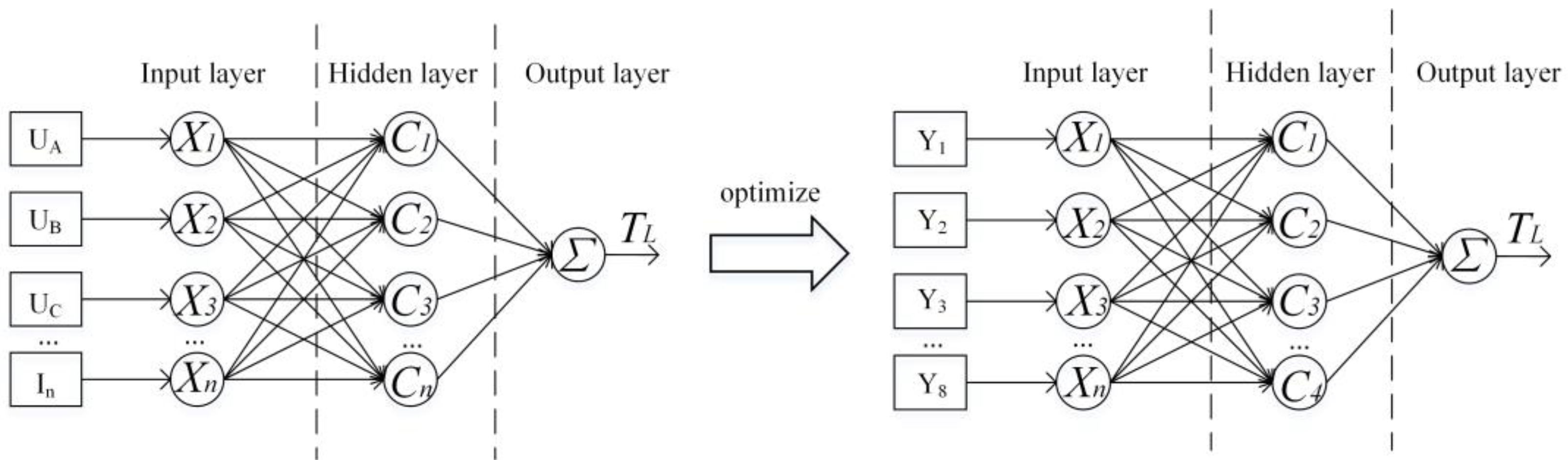
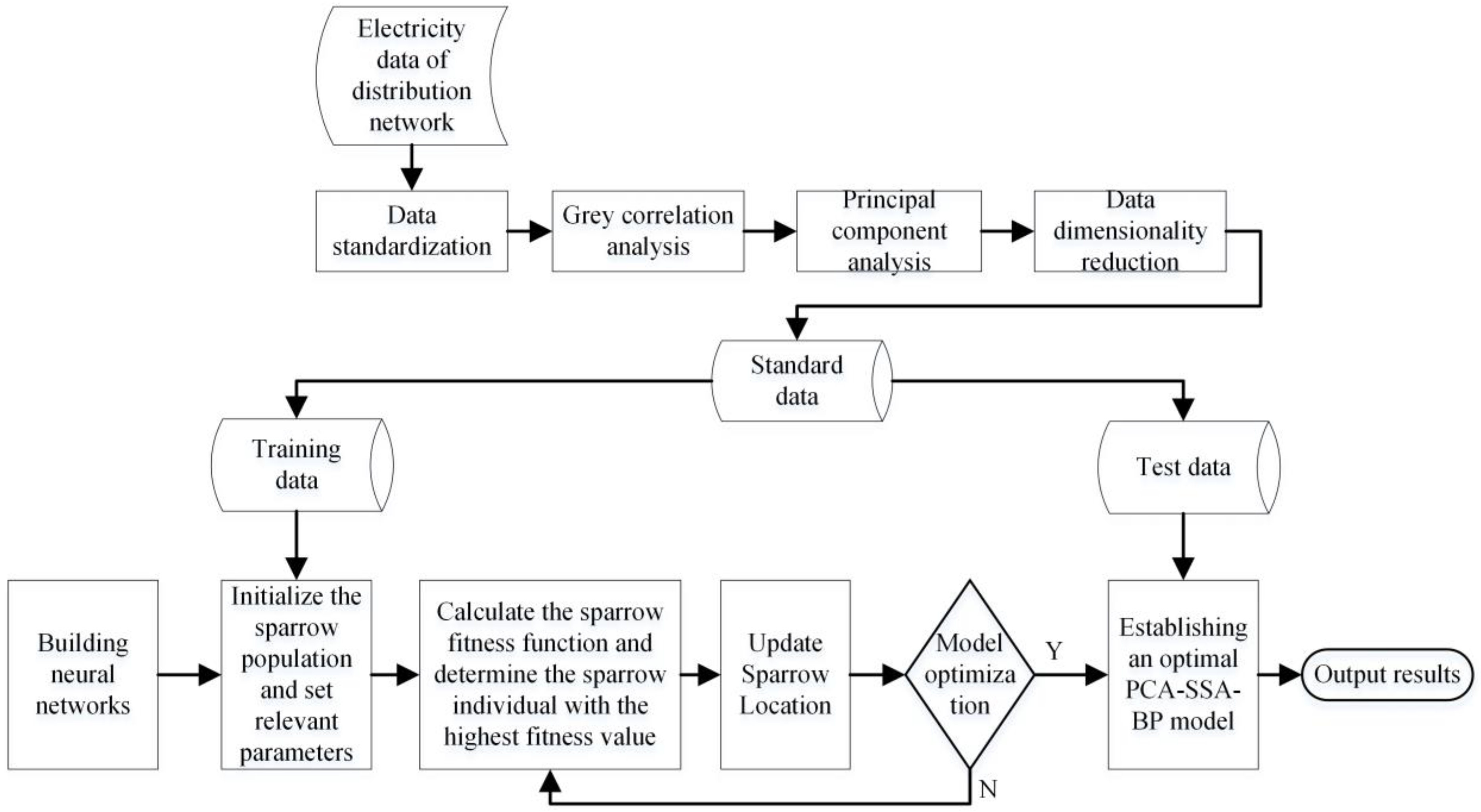
5. Modeling of Transformer Loss Based on PCA-SSA-BP

The total loss of the transformer can be calculated by using the zero-sequence impedance of the transformer, and then the transformer loss prediction model is trained by using the data detected by the distribution network and the total loss of the transformer. Although BP neural network can be optimized by using Sparrow Search Algorithm to seek the global optimal solution if SSA-BP neural network model is used for prediction directly, there is a strong correlation among the parameters, and it will lead to low accuracy of the model. The correlation among variables can be solved effectively by using Principal Component Analysis. By using Principal Component Analysis, the data collected from the distribution network z = {U_A, U_B, U_C, I_A, I_B, I_C, θ_A, θ_B, θ_C, I_n} are decreased to only eight principal components y = {Y₁, Y₂, Y₃, Y₄, Y₅, Y₆, Y₇, Y₈}. In the 2016 groups of data, the 1616 groups of data are used as the training samples, the 400 groups of data are used as test data and the accuracy is evaluated with average error. The input of network optimization is shown in Figure 1.

The modeling process of transformer loss prediction based on PCA-SSA-BP is shown in Figure 2.

The specific modeling process of the transformer loss prediction based on PCA-SSA-BP is described as follows:

• The original power data set detected in distribution network is {U_A, U_B, U_C, I_A, I_B, I_C, θ_A, θ_B, θ_C, I_n};
• The input dimension of the transformer loss prediction model is reduced by using Principal Component Analysis, expressed as {Y₁, Y₂, Y₃, Y₄, Y₅, Y₆, Y₇, Y₈};
• The 2016 groups of data detected in the distribution network are divided into two groups. The 1616 groups of data are used to train the transformer loss prediction model, and the 400 groups of data are used to test the established transformer loss prediction model;
• The initial size of sparrow population n is defined as n = 30, and the maximum number of iteration N is defined as N = 100.
• The topological structure of BP network and the search space dimension dim of sparrow search algorithm are determined, the input layer and hidden layer are defined as M and N, respectively, then the structure is M − N − 1, and the search dimension dim is M × N + N × 1 + N + 1;
• Then, the fitness function is determined. In this paper, the fitness function is defined as the average value of the mean square error of the training set and the mean square error of the test set. The function is shown in (30).

  $$\mathrm{fitness} =\frac{1}{2}\left(\frac{1}{{\mathrm{N}}_1}{\displaystyle \sum _{\mathrm{i}=1}^{{\mathrm{N}}_1}{\left({\mathrm{y}}_{\mathrm{train}(\mathrm{i})}-\mathrm{y}\right)}^2}+\frac{1}{{\mathrm{N}}_2}{\displaystyle \sum _{\mathrm{j}={\mathrm{N}}_1+1}^{\mathrm{N}}{\left({\mathrm{y}}_{\mathrm{test}(\mathrm{j})}-\mathrm{y}\right)}^2}\right),$$

  (30)

  where N₁ is the number of training sets, N₁ = 1616, N₂ is the number of test sets, N₂ = 400, N = N₁ + N₂; y_train is the output value of training set, y_test is the output value of test set and y is the actual value.
• The fitness values of the initial sparrow population are calculated and ranked, and the current corresponding best value f_best and the worst value f_worst are selected.
• The location of the discoverer, the joiner and the sparrow individuals who sense danger are updated according to steps (6) and (7).
• According to the iteration rules, if the current optimal value is better than the last iteration result, the update will continue, otherwise it will not be updated, and the iteration will continue.
• Set iteration termination criteria. When the fitness value is less than the accuracy of the initial model or the number of iterations is exhausted, the iteration will be terminated, and the optimal fitness value and its corresponding global optimal position best_x will be output.
• The BP network is optimized by using the global optimal position best_x, the optimal weight and threshold parameters are obtained and assigned to the BP network model, so as to realize training and simulation prediction of the network.

6. Example Verification

6.1. Verification of Zero-Sequence Impedance

According to the model and operation data of the transformer provided in [16], it is used to verify the correctness of the CGO algorithm. The specific information of the transformer is shown in

Table 9. Basic parameters of distribution transformer.

Type	Connection Layout	Capacity/kVA	Short Circuit Impedance/%	Rated Voltage/kV	Short Circuit Loss/W
S11	Yyn0	315	4	10/0.4	3830

. The comparison results are shown in

Table 10. Calculation results comparison of zero-sequence impedance.

Paper Data/Ω	Measured Data/Ω	Calculated Data/Ω	Error Percentage
0.094	0.087	0.094	8.44%
0.108	0.110	0.110	0.17%
0.112	0.112	0.113	0.90%
0.089	0.094	0.094	0.42%
0.103	0.109	0.106	2.57%

.

The percentage error in Table 10 is calculated by using (31).

$$\mathrm{E}\mathrm{r}\mathrm{r}\mathrm{o}\mathrm{r} \mathrm{p}\mathrm{e}\mathrm{r}\mathrm{c}\mathrm{e}\mathrm{n}\mathrm{t}\mathrm{a}\mathrm{g}\mathrm{e}=\left(\frac{\left(\mathrm{M}\mathrm{e}\mathrm{a}\mathrm{s}\mathrm{u}\mathrm{r}\mathrm{e}\mathrm{d} \mathrm{d}\mathrm{a}\mathrm{t}\mathrm{a}-\mathrm{C}\mathrm{a}\mathrm{l}\mathrm{c}\mathrm{u}\mathrm{l}\mathrm{a}\mathrm{t}\mathrm{e}\mathrm{d} \mathrm{d}\mathrm{a}\mathrm{t}\mathrm{a}\right)}{\mathrm{M}\mathrm{e}\mathrm{a}\mathrm{s}\mathrm{u}\mathrm{r}\mathrm{e}\mathrm{d} \mathrm{d}\mathrm{a}\mathrm{t}\mathrm{a}}\right)\times 100\%.$$

(31)

In addition to comparison of the zero-sequence impedance of the transformer, the three-phase voltage and neutral current of the transformer can also be compared, as shown in

Table 11. Calculated results comparison of transformer voltage.

A Phase Voltage/V	B Phase Voltage/V	C Phase Voltage/V	Three-Phase Voltage Source Value/V
243.10	233.60	237.50	238.87
240.40	234.00	228.70	235.27
242.70	237.20	231.40	237.88
237.10	232.50	230.50	234.46
238.70	233.40	233.40	235.96

and

Table 12. Calculation results comparison of neutral line current.

Paper Data/A	Calculation Data/A	Error Percentage
52.76	52.76	0.008%
60.46	60.39	0.111%
55.90	55.87	0.046%
42.00	42.10	0.248%
32.30	32.33	0.095%

.

From Table 10, Table 11 and Table 12, it can be seen that the error between calculated data and the measured data is very small. It proves the correctness of transformer calculated by the CGO algorithm.

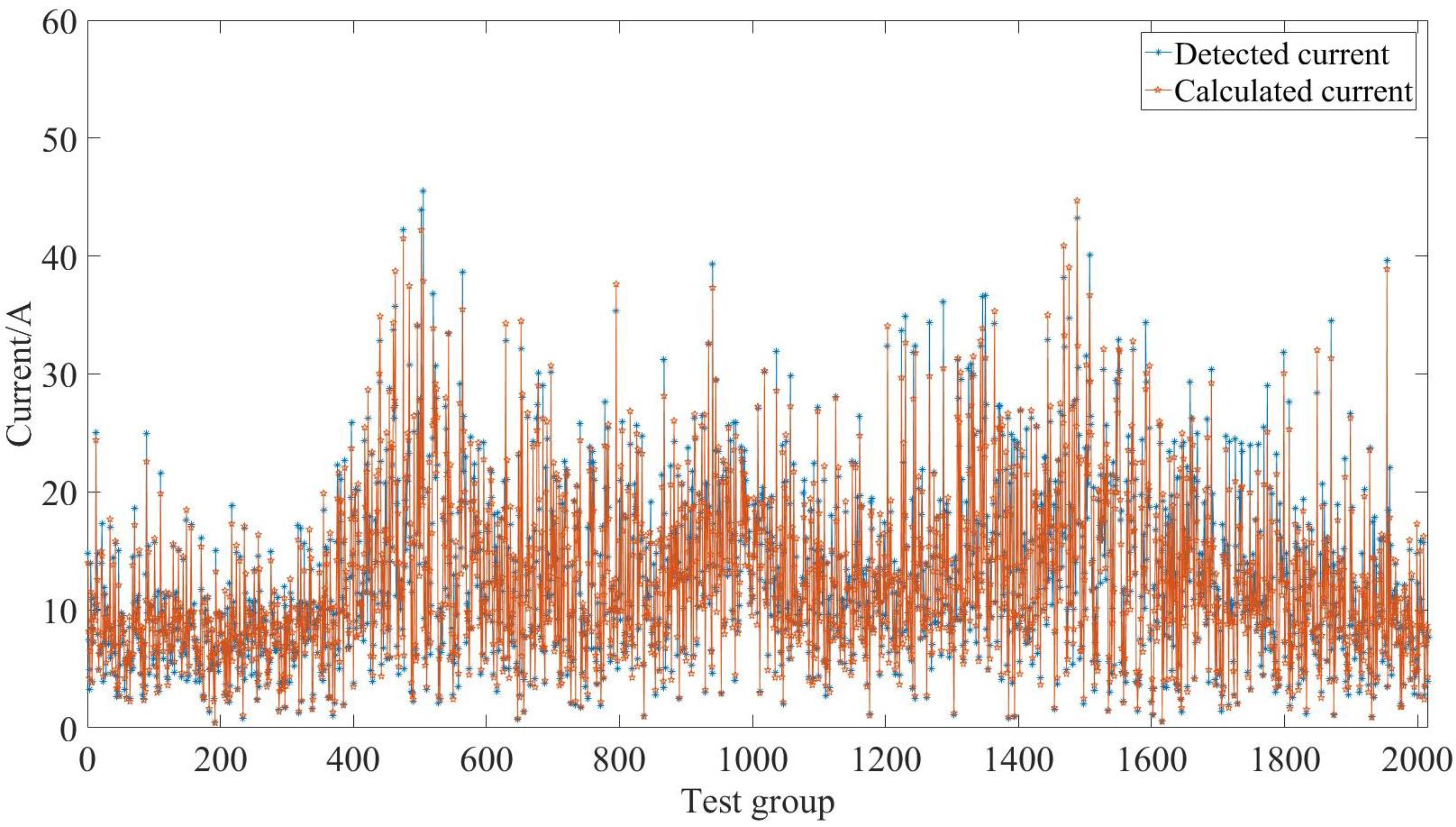
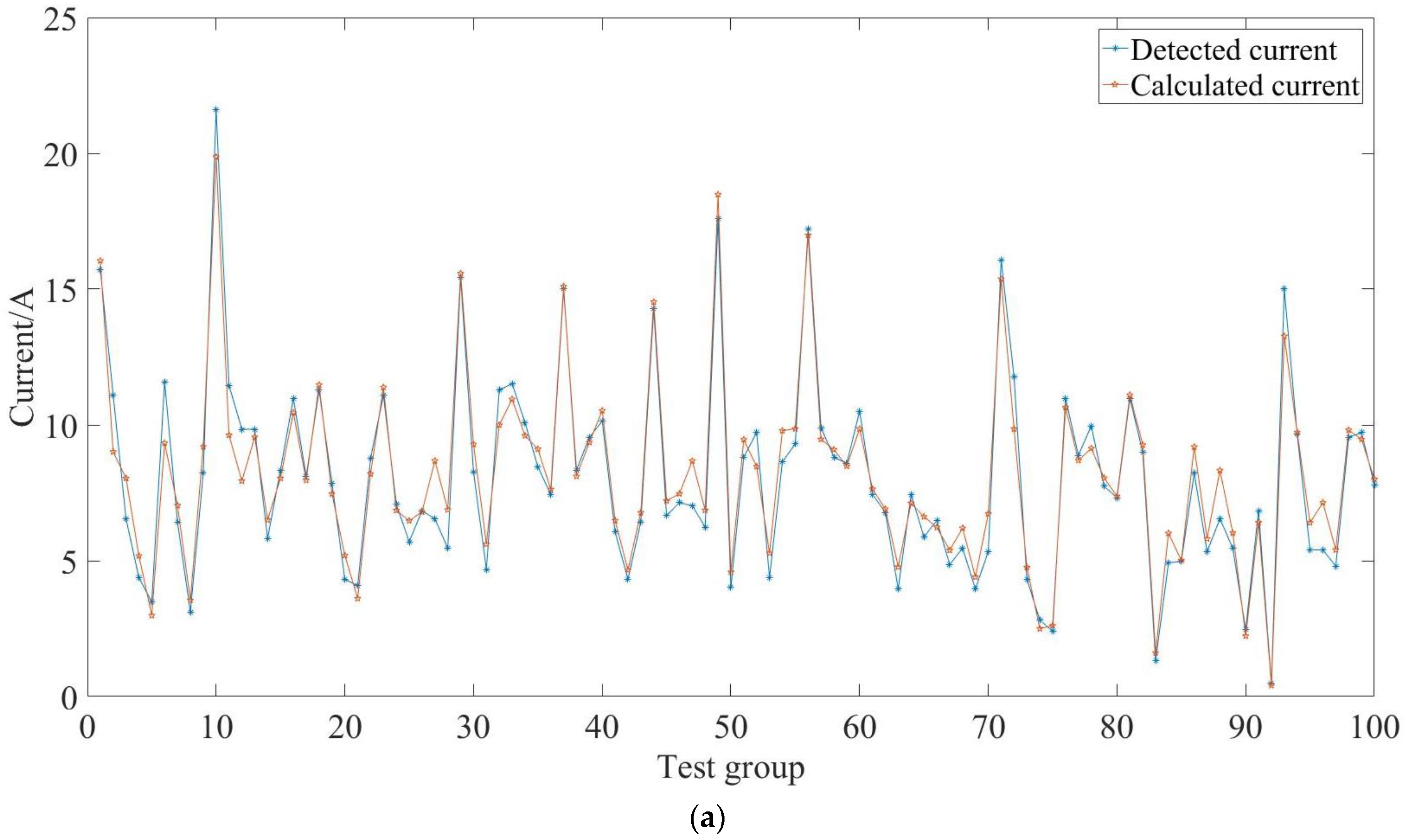
6.2. Verification of Neutral Line Current

The operation data of a transformer for 21 days provided by a power supply company in Liaoning Province is selected. For the normal operation of the transformer, the voltage, current and power data of the transformer should be detected every 15 min. So 96 groups of transformer data can be detected in a day, and there are 2016 groups of data in 21 days. The total loss of the transformer is regarded as the decisive factor. Partial operation data of distribution transformer are shown in Table 2. The specific information of the transformer is shown in

Table 13. Basic parameters of distribution transformer.

Type	Connection Layout	Capacity/kVA	Short Circuit Impedance/%	Rated Voltage/kV	Short Circuit Loss/W
S13	Dyn11	50	4	10/0.4	870

.

The voltage, current and power data detected in the distribution network can be written as 2016 groups of nonlinear equations, and each nonlinear equation is equivalent to an objective function, it is solved by CGO optimization algorithm. The comparison result between the neutral line current calculated by this algorithm and the actual detected is shown in Figure 3, and the error of the calculation result is shown in Figure 4.

As can be seen from Figure 4, the maximum error of the calculation results is less than 20%, and the average error percentage of the 2016 groups of data is 7.32%. Due to the large amount of data, the data from 1 to 100 and 101 to 200 are selected to observe, as shown in Figure 5.

As can be seen from Figure 5, the calculated current and the detected current have the same changes and the error is very small, it can prove the correctness of the CGO algorithm in calculating the neutral point current of the transformer.

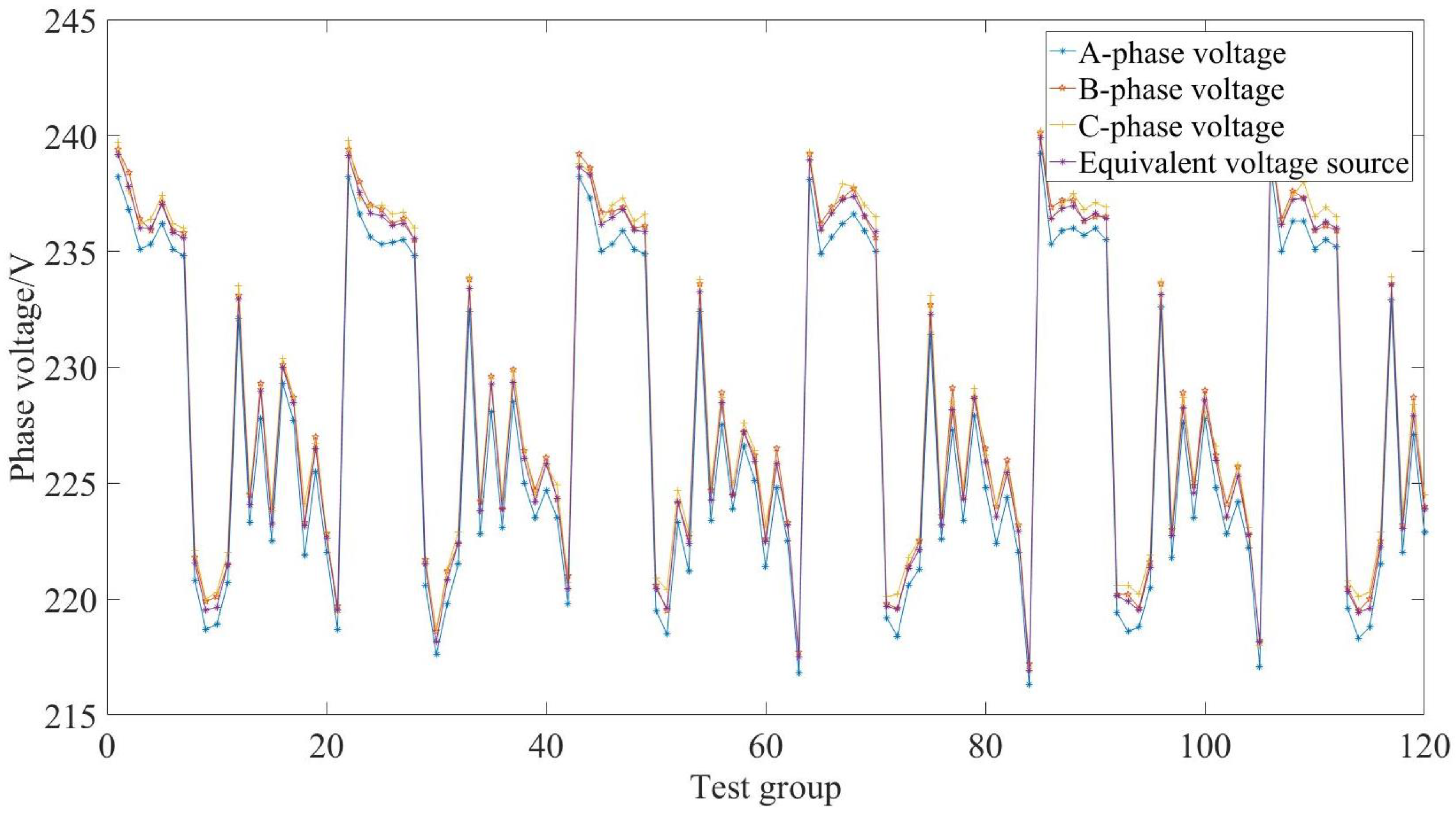
6.3. Verification of Transformer Voltage

The comparison diagram between the three-phase voltage source value calculated by the CGO algorithm and the three-phase voltage detected by the distribution network is now listed. The comparison diagram is shown in Figure 6.

There are 2016 groups of original electricity data. Due to the large amount of data, the 120 groups of voltage data are now listed. The comparison diagram is shown in Figure 7.

As can be seen from Figure 7, the changes of the three-phase voltage source of the transformer calculated by the CGO algorithm is consistent with the actual detected voltage, and the error is very small, it proves the correctness of the CGO algorithm in calculating the equivalent voltage source of the transformer.

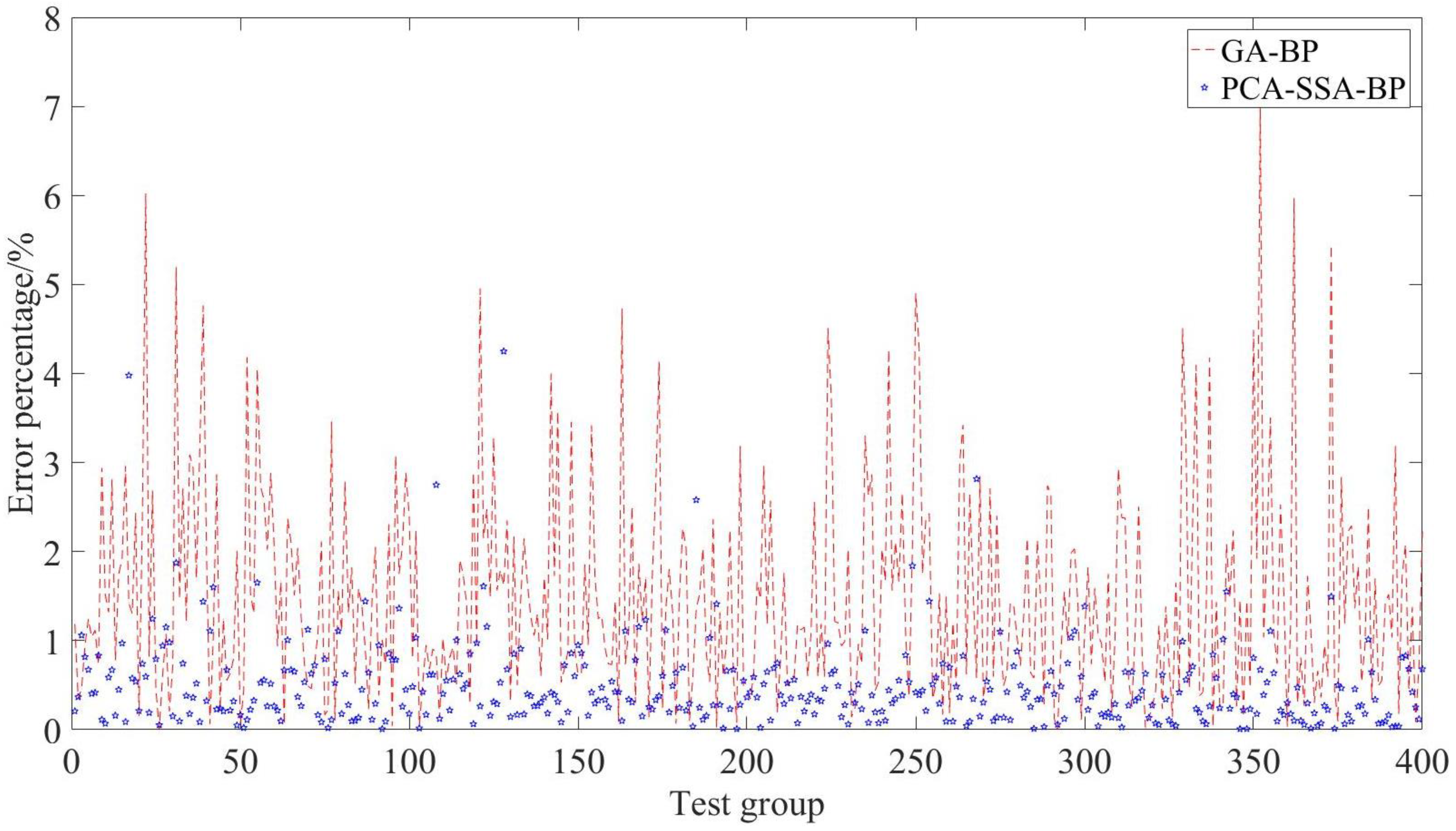
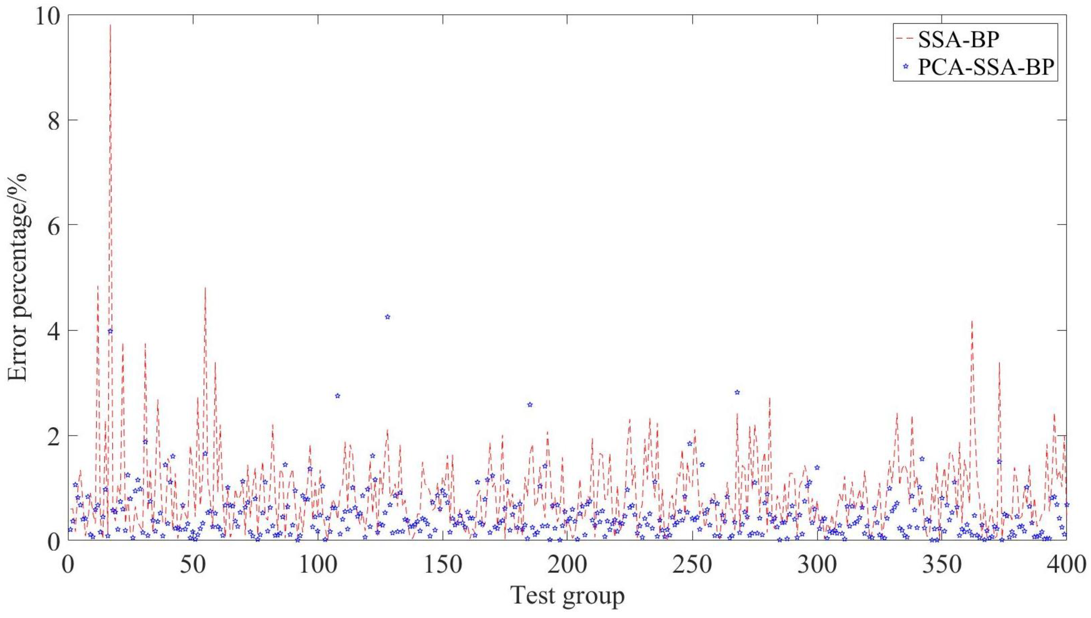
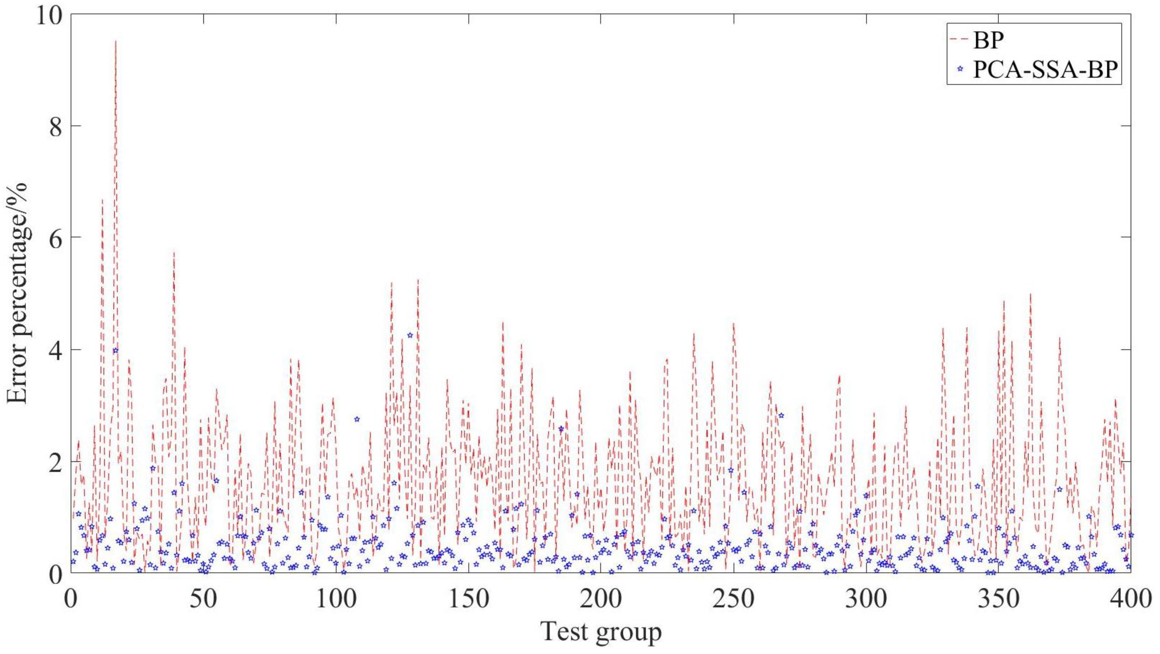
6.4. Intelligent Prediction of Transformer Loss Based on PCA-SSA-BP

In this paper, 1616 groups of data are used as training samples in the PCA-SSA-BP network, 400 groups of data are used as prediction data and the accuracy is evaluated by using the average error. To verify the effectiveness of this algorithm, this algorithm is compared with GA-BP, SSA-BP, BP and PSO-BP network prediction models. The comparison diagrams are shown in Figure 8, Figure 9, Figure 10 and Figure 11 below.

The average error percentages of transformer loss predicted by BP, GA-BP, PSO-BP, SSA-BP and PCA-SSA-BP neural networks are shown in

Table 14. Error comparison of predicting transformer loss for five algorithms.

Value	GA-BP	SSA-BP	BP	PSO-BP	PCA-SSA-BP
Minimum value	0.004%	0.003%	0.005%	0.001%	0.002%
Maximum value	7.035%	9.806%	9.515%	9.920%	4.250%
Median value	1.228%	0.765%	1.532%	1.005%	0.364%
Average value	1.64%	0.94%	1.75%	1.45%	0.63%

.

From Table 14, it can be seen that although the minimum error percentage of the PCA-SSA-BP model is not the smallest, the median and maximum error percentages are reduced compared to the other four algorithms. Therefore, the accuracy of the transformer loss prediction model can be improved by using PCA-SSA-BP. Compared with the transformer loss prediction model based on the BP network, the accuracy of the transformer loss prediction model based on PCA-SSA-BP has been improved by 1.12%; Compared with the transformer loss prediction model based on the GA-BP network, the accuracy of the transformer loss prediction model based on PCA-SSA-BP has been improved by 1.01%; Compared with the transformer loss prediction model based on PSO-BP network, the accuracy of transformer loss prediction model based on PCA-SSA-BP has been improved by 0.82%; Compared with the transformer loss prediction model based on SSA-BP network, the accuracy of transformer loss prediction model based on PCA-SSA-BP has been improved by 0.31%. The transformer loss prediction model based on PCA-SSA-BP is accurate by using 2016 groups of data. It is suitable for the loss estimation of power flow calculation in the distribution network.

7. Conclusions

An intelligent transformer loss prediction model based on PCA-SSA-BP is proposed to solve the problem of low accuracy in transformer loss calculation under three-phase unbalanced loads. The prediction model for transformer loss is optimized and an accurate transformer loss prediction model is obtained. Compared with the transformer loss prediction model based on the BP network, GA-BP network, PSO-BP network and SSA-BP network, the transformer loss prediction model based on the PCA-SSA-BP network has been proven to be accurate by using actual data. The highest improvement in prediction accuracy is 1.12%. The effectiveness and feasibility of this algorithm is verified in the transformer loss prediction with an unbalanced load.

References

1. Xie, F.; Yin, Z.; Luo, A.; Yuan, J. Prediction of Distribution Network Line Loss Based on Grey Relation Analysis and XGboost. In Proceedings of the 2021 IEEE 2nd International Conference on Big Data, Artificial Intelligence and Internet of Things Engineering (ICBAIE), Nanchang, China, 26–28 March 2021; pp. 279–284. [Google Scholar]
2. Li, G.; Li, J.; Li, L.; Yu, S.; Wang, N.; Pan, S.; Ding, H.; Su, Z. Research on the Influence of Distributed Photovoltaics on Distribution Network Voltage in Three-phase Unbalanced State. In Proceedings of the 2022 4th International Conference on Power and Energy Technology (ICPET), Beijing, China, 28–31 July 2022; pp. 715–720. [Google Scholar]
3. Wang, W.; Wang, W.; Song, S.; Hu, W.; Guo, Q. Study on Daily Line Loss Calculation Based on Operation Data and Resistance Characteristics of Low Voltage Distribution Transformer Area. In Proceedings of the 2021 International Conference on Power System Technology (POWERCON), Haikou, China, 8–9 December 2021; pp. 2093–2096. [Google Scholar]
4. Mikic, O.M. Variance-Based Energy Loss Computation in Low Voltage Distribution Networks. IEEE Trans. Power Syst. 2007, 22, 179–187. [Google Scholar] [CrossRef]
5. Fan, Y.; Jun, L.; Bingbing, L. Design and application of integrated distribution network line loss analysis system. In Proceedings of the 2016 China International Conference on Electricity Distribution (CICED), Xi’an, China, 10–13 August 2016; pp. 1–4. [Google Scholar]
6. Chen, B.; Xiang, K.; Yang, L.; Su, Q.; Huang, D.; Huang, T. Theoretical Line Loss Calculation of Distribution Network Based on the Integrated Electricity and Line Loss Management System. In Proceedings of the 2018 China International Conference on Electricity Distribution (CICED), Tianjin, China, 17–19 September 2018; pp. 2531–2535. [Google Scholar]
7. Guihong, F.; Jianbin, Z.; Shuqiu, G.; Bingyi, Z. Line Losses Analysis and Management System of Distribution Networks Based on Local Area Network. In Proceedings of the 2005 IEEE/PES Transmission & Distribution Conference & Exposition: Asia and Pacific, Dalian, China, 18 August 2005; pp. 1–4. [Google Scholar]
8. Feng, N.; Jianming, Y. Line losses calculation in distribution network based on RBF neural network optimized by hierarchical GA. In Proceedings of the 2009 International Conference on Sustainable Power Generation and Supply, Nanjing, China, 6–7 April 2009; pp. 1–5. [Google Scholar]
9. Wang, W.; Wang, J.; Song, S.; Hu, W.; Guo, Q. Distribution Network Monthly Line Loss Calculate and Improvement with Convolutional Neural Network. In Proceedings of the 2021 China International Conference on Electricity Distribution (CICED), Shanghai, China, 7–9 April 2021; pp. 1035–1039. [Google Scholar]
10. Huang, W.; Chen, J.; Liu, C.; Shi, W.; Lin, C.; Lyu, X.; Gao, H. Research on Line-Loss Correlation Analysis Technology of Distribution Network Based on Apriori Algorithm. In Proceedings of the 2020 5th Asia Conference on Power and Electrical Engineering (ACPEE), Chengdu, China, 4–7 June 2020; pp. 1399–1403. [Google Scholar]
11. Xu, Y. Optimization of BP artificial neural network regression prediction model based on Improved Sparrow search algorithm with Sine chaotic mapping and its application. In Proceedings of the 2021 IEEE International Conference on Emergency Science and Information Technology (ICESIT), Chongqing, China, 22–24 November 2021; pp. 231–234. [Google Scholar]
12. Yin, L.; Chen, A.; Wu, M. The Application of Grey Relational Analysis Model in the Detection of Communication Interrupt in Self-Organizing Network. In Proceedings of the 2014 Fourth International Conference on Instrumentation and Measurement, Computer, Communication and Control, Harbin, China, 18–20 September 2014; pp. 435–438. [Google Scholar]
13. Chen, J.; Dong, Q.; Ni, X.; Hu, M. Quantitative Analysis of Heavy Metal Components in Soil by Laser-Induced Breakdown Spectroscopy Based on Principal Component Analysis. In Proceedings of the 2019 18th International Conference on Optical Communications and Networks (ICOCN), Huangshan, China, 5–8 August 2019; pp. 1–4. [Google Scholar]
14. Allcock, R.; Haydock, L.; Holland, S. Calculation of zero phase sequence impedance for power transformers using numerical methods. IEEE Trans. Magn. 1995, 31, 2048–2051. [Google Scholar] [CrossRef]
15. Ramadan, A.; Kamel, S.; Hussein, M.M.; Hassan, M.H. A New Application of Chaos Game Optimization Algorithm for Parameters Extraction of Three Diode Photovoltaic Model. IEEE Access 2021, 9, 51582–51594. [Google Scholar] [CrossRef]
16. An, Y.; Fan, R.; Liu, B.; Deng, C.; Cai, M.; Lin, S. A method for calculating the zero sequence impedance of distribution transformers. Transformer 2018, 55, 1–4. [Google Scholar] [CrossRef]
Figure 1. Optimal input of transformer loss prediction model.
Energies 16 04432 g001
Figure 2. Transformer loss prediction model based on PCA-SSA-BP.
Energies 16 04432 g002
Figure 3. Comparison diagram of neutral point current.
Energies 16 04432 g003
Figure 4. Error percentage of calculated current.
Energies 16 04432 g004
Figure 5. Comparison diagram of partial neutral point current. (a) Comparison diagram of neutral point current from 1 to 100; (b) Comparison diagram of neutral point current from 101 to 200.
Energies 16 04432 g005aEnergies 16 04432 g005b
Figure 6. Voltage comparison diagram.
Energies 16 04432 g006
Figure 7. Partial voltage comparison diagram.
Energies 16 04432 g007
Figure 8. Error percentage of GA-BP and PCA-SSA-BP.
Energies 16 04432 g008
Figure 9. Error percentage of SSA-BP and PCA-SSA-BP.
Energies 16 04432 g009
Figure 10. Error percentage of BP and PCA-SSA-BP.
Energies 16 04432 g010
Figure 11. Error percentage of PSO-BP and PCA-SSA-BP.
Energies 16 04432 g011