Article

Comparing Machine Learning Strategies for SoH Estimation of Lithium-Ion Batteries Using a Feature-Based Approach †

Department of Electronics, Information and Bioengineering, Politecnico di Milano, 20133 Milan, Italy
*
Author to whom correspondence should be addressed.
This paper is an extended version of our paper published in the 18th IMEKO TC10 Conference on Measurement for Diagnostic, Optimization and Control to Support Sustainability and Resilience 2022, pp. 109–113.
Energies 2023, 16(11), 4423; https://doi.org/10.3390/en16114423
Submission received: 20 April 2023 / Revised: 16 May 2023 / Accepted: 19 May 2023 / Published: 30 May 2023
(This article belongs to the Special Issue Battery Modelling, Applications, and Technology)

Abstract

:
Lithium-ion batteries play a vital role in many systems and applications, making them the most commonly used battery energy storage systems. Optimizing their usage requires accurate state-of-health (SoH) estimation, which provides insight into the performance level of the battery and improves the precision of other diagnostic measures, such as state of charge. In this paper, the classical machine learning (ML) strategies of multiple linear and polynomial regression, support vector regression (SVR), and random forest are compared for the task of battery SoH estimation. These ML strategies were selected because they represent a good compromise between light computational effort, applicability, and accuracy of results. The best results were produced using SVR, followed closely by multiple linear regression. This paper also discusses the feature selection process based on the partial charging time between different voltage intervals and shows the linear dependence of these features with capacity reduction. The feature selection, parameter tuning, and performance evaluation of all models were completed using a dataset from the Prognostics Center of Excellence at NASA, considering three batteries in the dataset.

1. Introduction

One of the primary challenges of modern life is global warming caused by the emission of greenhouse gases from burning fossil fuels, as well as the urgency to diminish reliance on non-renewable resources. Renewable energy generation has become a top priority for governments all around the world. Focusing on photovoltaics (PVs) and wind, which are generally considered non-dispatchable and only partially participate in maintaining grid stability [1], makes battery and other energy storage systems essential. Out of the various battery technologies currently in use, lithium-ion batteries have become the preferred choice, owing to their high power and energy density as well as long service life [2]. For these reasons, exclusively Li-ion batteries are used in electric vehicles [3], where maximizing energy density and minimizing the weight of the battery pack is crucial. Continuous research and investments are focused on this technology to improve its performance, robustness, and stability.
A battery management system (BMS) is commonly used to ensure safe and efficient operation of the battery pack by controlling the charge and discharge processes of the cells and providing cell balancing. To achieve this task, the BMS must accurately estimate crucial battery parameters, such as state of charge (SoC), state of health (SoH), and the remaining useful life (RUL) [4]. The SoC is related to the available capacity of the batteries. By knowing this factor, the BMS prevents overcharging or discharging of batteries. The SoH provides information about the aging status of the battery and is indicated by the rise of internal resistance or capacity decrease. On the other hand, the goal of the RUL prediction is to understand how long a battery will continue to operate before it fails or has unacceptable performance. Battery degradation is a highly variable process, depending on cell chemistry, the BMS, ambient conditions, and use patterns. For this reason, a considerable amount of model-based [5,6,7,8,9] and data-driven battery aging methods used for the SoH and end-of-life predictions of batteries can be found in the literature.
Recently, data-driven methods have gained popularity due to the availability of vast amounts of data, gathered through sensors and other monitoring devices, and advancements in the field of machine learning (ML). They do not necessarily rely on prior knowledge of the particular battery cell and are less expensive to develop compared to the model-based ones. Data-driven methods use large data sets to identify patterns and relationships that may not be easily discernible using traditional analytical techniques. Many different features, otherwise known as health indicators (His), have been used to build various ML strategies. Apart from capacity and resistance changes, these His are based on voltage charge–discharge limits, the amount of current, battery temperature [10,11,12,13,14], and incremental capacitance analysis (ICA) [15,16,17,18], as well as features derived from statistical analysis of the other health indicators [19].
In the literature, many machine learning techniques have been studied and used to perform SoH estimation [20,21] apply regression to model battery aging behavior and compare the RUL-prediction capabilities of two fitting functions, while in [22], a combination of an exponential function and regression analysis is used. The authors of [23] discuss a strategy based on support vector regression (SVR) and ICA curves obtained from partial charging data. Similarly, [14] uses partial charging segments of voltage under constant current charging and a support vector machine model. Another SVR strategy is presented in [24], based on curves of battery voltage as a function of charging capacity (V-Q). Finally, in [25], a solution is proposed based on the random forest algorithm. In [13], a gaussian process regression (GPR) model is used with four specific inputs extracted from the charging curves, and a grey relational analysis method is applied to analyze the relationship between features and SoH. The authors of [26] apply GPR to discover the relationship between capacity, storage temperature, and SoC of lithium-ion batteries. By optimizing the feature selection process with an automatic-relevance-determination (ARD) structure, they provide predictions for the calendar aging of batteries tested under different conditions. GPR combined with electrochemical impedance spectroscopy is used in [27], adopting many wave shapes to obtain an estimation of the capacity of the batteries. Novel health indicators related to the lithium diffusion coefficient are provided and validated.
In [28], a capacity-estimation method based on back-propagation neural networks (NN) and partial charging voltage segments, corresponding to 10–50% SOC, has been developed. Another solution based on recurrent neural networks (RNNSs) is proposed in [29], while in [30], an echo state network (ESN) has been used together with a model-based approach to predict the SoH evolution curve of the tested batteries, starting from cycles 80, 100, or 120. From the generated curves, predictions are made for the RUL. Due to the problem of vanishing or exploding gradient, traditional RNNs are not capable of dealing with long sequences in practice. The emergence of long short-term memory (LSTM) has provided a solution to this problem [31], and [32] utilized LSTM to build a RUL model of the lithium-ion battery. In [33], another method is proposed based on LSTM NNs and signal processing methods for SoH monitoring and RUL prediction of lithium-ion batteries.
In [34], the authors proposed an approach for SoH estimation based on SVR and a feature extraction procedure. In this paper, SVR is compared to other ML approaches, including multiple linear and polynomial regression and random forest. These classical ML strategies have been chosen because they offer a good compromise between light computational effort, applicability, and accuracy of results, while also providing higher model interpretability than complex NNs. The performances of all strategies are compared using a dataset from the Prognostics Center of Excellence at NASA, considering three batteries of the dataset. This work differentiates itself from the other aforecited papers, including the ones employing the same NASA dataset [10,11,12,13,18,28,30,33], based on the specific ML strategies implemented, the features used, and their feature numbers. Discussion is provided on the feature selection process based on partial charging times between different voltage limits, as well as the parameter tuning process of the different strategies. Finally, this research had the goal of minimizing the necessary number of features, considering models based on one-to-four features, and achieving optimal results with only two features for all considered ML strategies.

2. NASA Dataset

The NASA Ames Prognostics Center of Excellence (PCoE) released a data repository composed of six datasets of aged Li-ion batteries [35]. However, only the first of these datasets is suitable for prognostic degradation prediction, according to their guidelines. In this work, batteries 5, 6, and 7 were considered, which were tested until failure. The charging process follows the constant-current (CC) and constant-voltage (CV) protocol. More specifically, the cells are charged with a current of 1.5 A until the upper voltage limit of 4.2 V is met, after which CV charging proceeds until the current drops below 20 mA. The discharge phase is carried out at 2.7 V, 2.5 V, and 2.2 V, depending on the battery. Cycles are grouped into charge, discharge, or impedance cycles. For every cycle of every cell, various quantities are measured, including current, time, temperature, voltage, and discharge capacity. To control the environmental temperature, the tests were carried out in a climatic chamber.

3. Considered Machine Learning Strategies

3.1. Multiple Linear Regression and Stepwise Regression

Multiple linear regression (MLR) is a statistical approach for modeling the relationship between a target variable (y) and two or more available descriptor variables (xi), otherwise called features, using a linear equation. Regression models are usually fitted using the least-squares approach, which minimizes the sum of the squared differences between the predicted and actual values of the target variable. However, fitting based on other criteria can be performed, such as least absolute deviations or minimization of a penalized version of the least-squares function, as in the case of ridge and lasso regression. MLR is a powerful tool for analyzing complex relationships between variables, but it assumes that the relationships are linear. When this is not the case, better results could be obtained using polynomial regression, which is a statistical technique that models the relationship between xi and y as an n-th degree polynomial, thus fitting a nonlinear relationship. Polynomial regression utilizing multiple features can have many potential terms resulting from the features raised to a certain power or their combination.
Stepwise regression can be used to automatically identify the most important terms. It involves iteratively adding or removing different terms according to a stopping criterion, which can be based on the p-value, Akaike information criterion (AIC), Bayesian information criterion (BIC), value of the coefficient of determination (R2), or adjusted R2. The most popular stepwise methods are forward selection (FS), backward elimination (BE), and bidirectional elimination. In FS, the model starts with no terms and iteratively adds them until a stopping criterion is met. In BE, the model starts with all combinations and iteratively removes terms until a stopping criterion is met. For both the BE and the FS methods, the decision regarding a term is final and is not reconsidered. This is not the case with bidirectional elimination, which is a combination of forward and backward stepwise regression and starts with no terms. If the adjusted R2 is considered as a stopping criterion, this method will first add the terms that produce the largest increase in the adjusted R2 value. Eventually, the removal of terms can also occur if this results in maximum increases of the adjusted R2.
In this work, models based on MLR, as well as second- and third-degree polynomial terms, have been constructed using bidirectional-elimination stepwise regression. The generated models based on stepwise regression were limited to second- and third-degree polynomial terms, including combinational terms. The adjusted R2 was used as the stopping criterion. In all cases, fitting was performed by using the least-squares method.

3.2. Support Vector Regression

The support vector machine (SVM), in ML, is a well-known supervised learning model, used mainly for binary classification tasks. It has been extensively applied in predictive and diagnostic tasks, such as in [36], where a partial-discharge-curve approach is combined with the least-squares SVM to estimate the state of health (SoH) of Li-ion batteries. Similarly, in [37], the SVM is utilized on an electric-vehicle (EV) battery-usage-profile dataset generated by simulations to determine the SoH. The SVM searches for the optimal hyperplane that maximizes the distance from each training point, making it not only effective in classifying points but also in finding the most robust hyperplane. When the points are not linearly separable and a higher-dimensional feature space is needed, the kernel trick is used.
SVR is a version of the SVM adapted to perform regression tasks. SVR fits the error of its predictions within the limit ϵ while minimizing the loss function in Equation (1), which is called the L2 loss:
min 1 2 β β Y n ( X n β + b ) ϵ n
where
β , β —values that weight arrays, normal and transposed
Y n —target values
X n —transposed descriptor array
b —bias
ϵ —maximum allowed error.
The ϵ constraint is then relaxed, introducing the slack variables and applying what is called the soft margin approach.
min 1 2 β β + C n = 1 N ( ξ n + ξ n * ) Y n X n β + b ϵ + ξ n n X n β + b Y n ϵ + ξ n * n
where
ξ n , ξ n * —slack variables for positive and negative error
C—weight associated with slack variables.
The prediction is expressed as a function of the training samples in Equation (3), in particular of those data points with either αi or α i * different from 0, which are called support vectors.
β = n = 1 N α n α n * X n f x = n = 1 N α n α n * ( X n X ) + b
In this paper, the SVR hyperparameters have been initially tuned with the MATLAB built-in function for SVR models, using the Bayesian optimization algorithm, and run for 500 iterations to define a good starting point for the hyperparameters. The tunable hyperparameters are as listed:
Box constraint: Coefficient C that weights the slack variables in Equation (1) and helps regulate overfitting.
Epsilon (ε): The value that defines the radius of the epsilon tube where the algorithm tries to contain the points or, in other words, the maximum error allowed.
Kernel scale: The value that rescales the predictors. Each value in the predictors is divided by the kernel scale value.
Kernel function: The value used to compute the similarity between data points in a higher-dimensional feature space.
Additional tuning of the hyperparameters was carried out during the validation process. The final values of the hyperparameters are shown in Table 1. The linear kernel function was selected because the features are quite proportional to the target value to estimate and working in a higher-dimensional space was unnecessary. In fact, different kernel functions led to lower validation accuracy.

3.3. Random Forest

A random forest (RF) is an ensemble learning method that puts together many decision trees (DT) as weak learners and is one of the best-known and most used algorithms for supervised learning tasks. In [38], a RF is used to perform an incremental capacity analysis to estimate the capacity of lithium batteries by only feeding raw measurements of new data to the model.
A decision tree is a non-parametric algorithm that develops a tree by splitting the dataset over the values of its features and associates different subsets of the dataset to different nodes of the tree. First, the entire dataset is paired with the root of the tree. Next, the dataset is split into two parts according to a decision made over some of the features, and each part is associated with a new node child of the root, forming the second level of the tree. This behavior is recursively iterated until subsets of the dataset contain only one value or a stop criterion is met, with the final subsets representing the leaves of the tree. Each splitting is made over the value of typically one feature, and the choice for the optimal split is made by finding the feature and its splitting value that optimize a given metric. MSE metric minimization was used in this work:
M S E S = 1 N i = 1 N y i y ¯ 2 s p l i t M S E F , V = N L N M S E S L + N R N M S E S R F * , V * = a r g m i n ( s p l i t M S E F , V )
where y ¯ is the mean of the target values in the set S, yi is the i-th target value, and N is the number of samples in the set. SplitMSE, SL, and SR are the weighted error, left, and right subsets, respectively, generated by splitting S over the feature F at value V, while NL and NR are the numbers of data points, respectively, in the left and right subsets. F* and S* are the optimal feature-value pair to split the set. Other metrics, such as Gini impurity or information gain, can be used.
However, decision trees are considered weak learners and strongly tend to overfit. A random forest is an ensemble algorithm whose mechanism consists of combining multiple decision trees with a bagging technique to provide higher accuracy and robustness than a single tree, reducing overfitting. Bagging is, in fact, known for reducing the variance of the model (as opposed to boosting, which reduces bias) by training each tree (or learner in general) on a randomly selected subset of the training data with replacement (bootstrapping), hence introducing diversity in the training data. What diversifies the random forest from the standard tree bagging ensemble is the use of subsets of randomly selected features for each tree in the forest, which helps to reduce correlation between each learner, thus reducing overfitting. In this work, one-third of the total features were randomly used to train each single decision tree.

4. Feature Selection

As aforementioned, the considered approaches were applied by considering a specific feature of the batteries. In most battery applications, the charging stage is conducted in a more repeatable way. While different chargers can be used, which will result in different charging profiles, many charging cycles will be the same or very similar. On the other hand, the battery discharge cycles vary greatly depending on the application and use patterns. Even though the charging phase is more similar between different cycles, complete charging cycles are by no means guaranteed. For this reason, a small portion of the charging curve of voltage was used to extract useful information. More specifically, the extracted feature is the partial charging time (PCT) necessary for the battery to charge by some small voltage range.
In Figure 1, the battery voltage versus time during charging for different cycles is represented. Unsurprisingly, the charging time decreases as the battery ages and the global capacity decreases. In fact, the charging time is halved near the final cycles compared to the initial ones. It is further noted that the beginning of the charging process is characterized by a high derivative and is therefore difficult to appreciate the time differences between different cycles. On the other hand, the middle part extends for a longer period of time and is more suitable for PCT feature extraction. This is why, in this work, the lower voltage limit of 3.7 V was set for the feature extraction process.

5. Results and Discussion

The initial choice of the voltage range and limits was made empirically by computing four features over the limits of 3.7–4.1 volts with a voltage range of 0.1 V. More specifically, the first feature represents the evolution of the charging time between 3.7 V and 3.8 V over the number of cycles, the second feature uses the range of 3.8 V to 3.9 V, etc. In Figure 2, the value of the considered features as a function of the number of cycles is plotted. The first PCT feature computed for the lowest voltage values, from 3.7 V to 3.8 V, appeared to be an almost flat curve, containing no variance and thus very little information regarding the data. Conversely, the features computed from 3.8 V to 4.1 V have a higher variance and hence are more descriptive of the aging phenomena.
To find the optimal features and model parameters, from the voltage limits of 3.7–4.1 V, many feature sets were created. These sets differ from each other depending on the number of features, the upper and lower voltage limits used, and the voltage range. For each feature set, the models obtained using the different ML strategies are compared.
The fitting accuracy of the various models was assessed through the value of the coefficient of determination (R2). It is a measure used in statistics, indicating how much a hypothesis describes the variance of the data. In other words, it is a measure of how well a model can fit the data. R2 is described as
R 2 = 1 S S r S S t S S r = i y i f i 2 S S t = i y i y ¯ 2
where
S S r —residual sum of squares
S S t —total sum of squares
y i —target value
f i —estimated value
y ¯ —mean of the target values.
A three-fold cross-validation (CV) procedure was applied to the three batteries of the dataset to find the best features and ML strategies. This means the SoH evolution of each battery was estimated based on the data of the other two batteries. The results are shown in Table 2 and Table 3 for the voltage ranges of 0.1 V and 0.05 V, respectively. Initially, a smaller voltage range of 0.025 V and a larger voltage range of 0.2 V were also considered. However, the smaller voltage range resulted in features with low variability for most voltage limits and produced inferior results compared to the ones presented in Table 2 and Table 3. The larger range of 0.2 V and higher ranges did not improve the SoH-estimation capability of the models. Since minimizing the voltage range was one of the objectives to ensure that the features would be available, even in the case of partial charging cycles, the ranges of 0.05 V and 0.1 V were regarded as optimal, and the higher voltage ranges were not further analyzed or presented.
Table 2 shows the feature sets of partial charging times obtained for a voltage range of 0.1 volts. The first four single feature sets (A1–A4) explore the whole voltage range of 3.7 to 4.1 volts. Unsurprisingly, they show that all ML strategies perform better when the voltage limits of 3.8–3.9 V (A2) or 3.9–4 V (A3) are used as a feature. More specifically, the best results are obtained for the voltage limits 3.9–4 V when a single feature is used. Additionally, Table 2 shows that if the feature set is built from two features based on the limits of 3.8–3.9 V and 3.9–4 V (A6), there is only a marginal improvement in the R2 value. In any case, the best results for single and double feature sets are A3 and A6.
Table 3 presents the feature sets obtained for a voltage range of 0.05 volts. In this case, feature sets consisting of one to four features were constructed. For example, B1 is a feature set of a single feature, which is the PCT between the voltage limits of 3.8 V to 3.85 V, while B6 consists of two features, which are the PCTs between the limits of 3.8 to 3.85 V and 3.85 to 3.9 V. The best results, per number of features, are B3, B7 B10, and B14. Using a single feature, even for the voltage range of 0.05 V, is sufficient if the voltage limits are between 3.85 and 4 volts. There is marginal improvement when two features are used; however, a further increase in the number of features does not lead to any meaningful increase of R2. Considering the models of both tables, it can be noted that SVR delivers slightly better results than the other considered ML strategies for all feature sets. Still, using MLR also leads to satisfactory results. Furthermore, when comparing the three strategies based on regression, no significant improvement in the R2 value is observed when increasing the polynomial order using stepwise regression. That means the PCT features and capacity reduction, as functions of the number of cycles, have a strong linear dependence. Hence, high model complexity will not result in an improvement of the results if the correct voltage range of 3.8–4 V has been selected. Actually, a drop in the mean validation R2 value can even be observed in some cases due to overfitting the training data of the higher-complexity models. This is especially apparent in models built from a higher number of features (A7 and B12 to B14). However, some improvement when increasing the polynomial order can also be observed for the voltage range of 3.7–3.8 V, which has low variance. Finally, the models based on RF demonstrated worse performance than those of MLR and SVR.
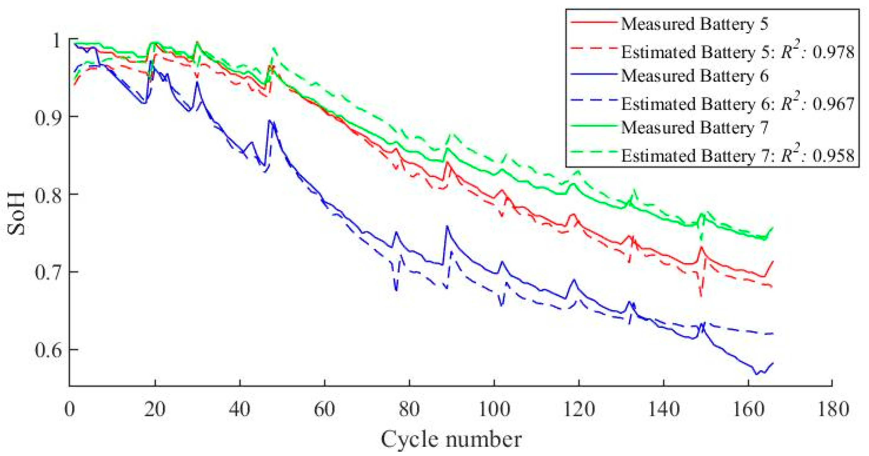
The models based on feature sets A3, A6, B3, B7, B10, and B14 all represent satisfactory performance. Having the goal of minimizing the number of features and the voltage range, the authors consider the models based on feature set B7 as the overall best. The plots for the capacity estimation of all the batteries using MLR, SVR, and RF are plotted in Figure 3, Figure 4 and Figure 5, respectively.
All three figures display the previously mentioned three-fold CV. For example, the SoH estimation of battery 5 was done with a model trained using the data of the chosen feature set of batteries 6 and 7. The full lines represent the measured SoH for the batteries, while the dashed lines represent the estimated SoH over the number of cycles. Figure 3 and Figure 4 show that MLR and SVR accurately model the SoH of the batteries, even registering the peaks in the SoH function that are due to the rest time of the battery. Likewise, the RF is able to model batteries 5 and 7 with similar success, but the same cannot be said about battery 6, as is evident in Figure 5. After the SoH of battery 6 falls to around 0.7, the estimation begins to diverge from the measurement because batteries 5 and 7, which were used for training, do not contain data with SoH lower than 0.7.
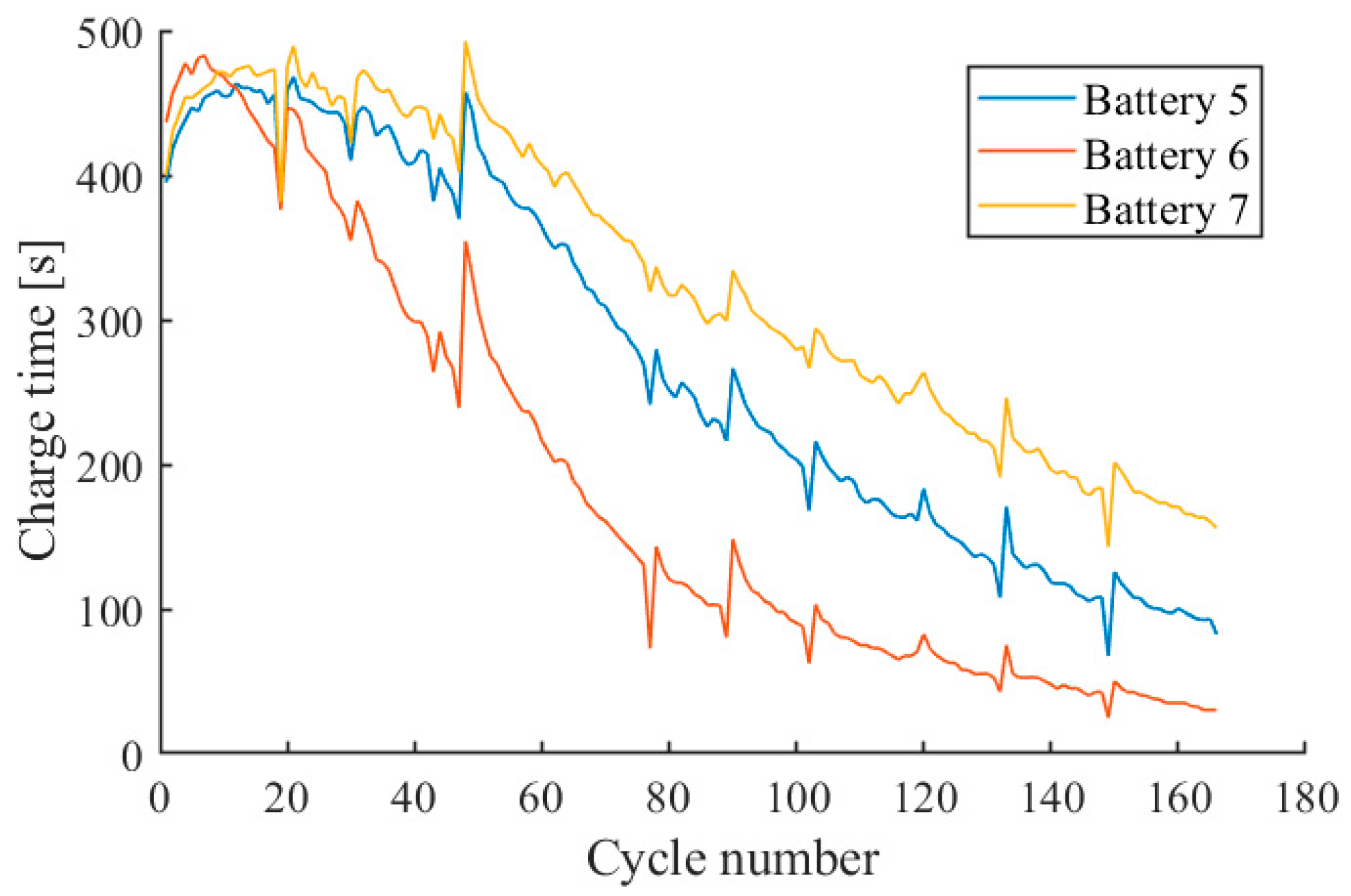
The random forest and decision trees are indeed well known for their inability to extrapolate, that is, make estimations for predictor values lying outside of the range of the observed data. From Figure 5, it is clear that the SoH value of battery 6 from cycle 90 onwards is lower than that of any other cycle of the training batteries; hence, the decision trees will not be able to correctly estimate that target value. Furthermore, Figure 6 shows that also the feature value for battery 6 is lower than that of the other batteries. Consequently, the branches of the decision trees built on batteries 5 and 7 will “explore” the features in a range that does not include the values of battery 6 predictors after cycle 90. Hence, after this cycle number, all the decision trees of the random forest will infer the lowest observed SoH value for battery 6, which will be around 0.7 because the training data is composed of batteries 5 and 7. This is the reason for the observed flat line output. It is important to specify that this result does not imply that the RF is not a suitable solution for the general problem of battery prognostic because this precise case is strictly related to the dataset distribution and data scarcity.

6. Conclusions

Accurate SoH estimation is essential for the safe and reliable operation of lithium-ion batteries. This paper compares SoH-estimation models based on the classical ML strategies of MLR, polynomial regression, SVR, and RF, which offer good trade-offs between applicability, light computation effort, and accuracy of results. Discussion is provided on the feature selection process and optimal number of features.
The partial charging time proved to be a good indicator of battery aging as long as the proper voltage limits were selected, and the partial charging phase was equal at every cycle. To find the optimal features, 21 feature sets were built considering different voltage limits and the two voltage ranges of 0.1 and 0.05 V. The best results were obtained when considering the voltage limits of 3.8 to 4 volts for both ranges of 0.1 V and 0.05 V. The quality of the features degrades significantly for a minimum voltage of less than 3.7 V due to small variance. Results showed that models based on one or two features are optimal.
Furthermore, the PCT feature demonstrated a linear dependence with capacity reduction as a function of number of cycles. Consequently, MLR produced very accurate results, and the use of polynomial regression was not justified. The overall best performance for all feature sets was achieved using SVR, especially when slightly lower voltage limits were considered. Finally, the RF had the worst performance when facing the limited dataset.

Author Contributions

Conceptualization, E.P., I.M. and L.C.; methodology, E.P. and I.M.; software, I.M. and E.P.; validation, I.M. and M.F.; formal analysis, E.P.; investigation, I.M.; resources, I.M.; data curation, L.C.; writing—original draft preparation, E.P. and I.M.; writing—review and editing, E.P. and I.M.; visualization, I.M.; supervision, L.C., M.F. and E.P.; project administration, L.C. and M.F.; funding acquisition, L.C. and M.F. All authors have read and agreed to the published version of the manuscript.

Funding

This research received no external funding.

Data Availability Statement

Not applicable.

Conflicts of Interest

The authors declare no conflict of interest.

References

  1. Cristaldi, L.; Faifer, M.; Laurano, C.; Ottoboni, R.; Petkovski, E.; Toscani, S. Power Generation Control Algorithm for the Participation of Photovoltaic Panels in Network Stability. IEEE Trans. Instrum. Meas. 2023, 72, 1–9. [Google Scholar] [CrossRef]
  2. Pelletier, S.; Jabali, O.; Laporte, G.; Veneroni, M. Battery Degradation and Behaviour for Electric Vehicles: Review and Numerical Analyses of Several Models. Transp. Res. Part B Methodol. 2017, 103, 158–187. [Google Scholar] [CrossRef]
  3. Werling, T.; Geuting, P.; Höschele, P.; Ellersdorfer, C.; Sinz, W. Investigation of the Electro-Mechanical Behavior of Automotive High Voltage Busbars under Combined Electrical Load with Varying Indenter Geometry and Environmental Conditions. J. Energy Storage 2020, 32, 101861. [Google Scholar] [CrossRef]
  4. Campestrini, C.; Horsche, M.F.; Zilberman, I.; Heil, T.; Zimmermann, T.; Jossen, A. Validation and Benchmark Methods for Battery Management System Functionalities: State of Charge Estimation Algorithms. J. Energy Storage 2016, 7, 38–51. [Google Scholar] [CrossRef]
  5. Tanim, T.R.; Rahn, C.D.; Wang, C.Y. A Temperature Dependent, Single Particle, Lithium Ion Cell Model Including Electrolyte Diffusion. J. Dyn. Syst. Meas. Control Trans. ASME 2015, 137, 011005. [Google Scholar] [CrossRef]
  6. Li, X.; Fan, G.; Rizzoni, G.; Canova, M.; Zhu, C.; Wei, G. A Simplified Multi-Particle Model for Lithium Ion Batteries via a Predictor-Corrector Strategy and Quasi-Linearization. Energy 2016, 116, 154–169. [Google Scholar] [CrossRef]
  7. Petit, M.; Prada, E.; Sauvant-Moynot, V. Development of an Empirical Aging Model for Li-Ion Batteries and Application to Assess the Impact of Vehicle-to-Grid Strategies on Battery Lifetime. Appl. Energy 2016, 172, 398–407. [Google Scholar] [CrossRef]
  8. Barcellona, S.; Colnago, S.; Dotelli, G.; Latorrata, S.; Piegari, L. Aging Effect on the Variation of Li-Ion Battery Resistance as Function of Temperature and State of Charge. J. Energy Storage 2022, 50, 104658. [Google Scholar] [CrossRef]
  9. Xu, B.; Oudalov, A.; Ulbig, A.; Andersson, G.; Kirschen, D.S. Modeling of Lithium-Ion Battery Degradation for Cell Life Assessment. IEEE Trans. Smart Grid 2018, 9, 1131–1140. [Google Scholar] [CrossRef]
  10. Cui, Z.; Wang, C.; Gao, X.; Tian, S. State of Health Estimation for Lithium-Ion Battery Based on the Coupling-Loop Nonlinear Autoregressive with Exogenous Inputs Neural Network. Electrochim. Acta 2021, 393, 139047. [Google Scholar] [CrossRef]
  11. Liu, D.; Zhou, J.; Liao, H.; Peng, Y.; Peng, X. A Health Indicator Extraction and Optimization Framework for Lithium-Ion Battery Degradation Modeling and Prognostics. IEEE Trans. Syst. Man. Cybern. Syst. 2015, 45, 915–928. [Google Scholar] [CrossRef]
  12. Cao, M.; Zhang, T.; Wang, J.; Liu, Y. A Deep Belief Network Approach to Remaining Capacity Estimation for Lithium-Ion Batteries Based on Charging Process Features. J. Energy Storage 2022, 48, 103825. [Google Scholar] [CrossRef]
  13. Yang, D.; Zhang, X.; Pan, R.; Wang, Y.; Chen, Z. A Novel Gaussian Process Regression Model for State-of-Health Estimation of Lithium-Ion Battery Using Charging Curve. J. Power Sources 2018, 384, 387–395. [Google Scholar] [CrossRef]
  14. Feng, X.; Weng, C.; He, X.; Han, X.; Lu, L.; Ren, D.; Ouyang, M. Online State-of-Health Estimation for Li-Ion Battery Using Partial Charging Segment Based on Support Vector Machine. IEEE Trans. Veh. Technol. 2019, 68, 8583–8592. [Google Scholar] [CrossRef]
  15. Tian, J.; Xiong, R.; Yu, Q. Fractional-Order Model-Based Incremental Capacity Analysis for Degradation State Recognition of Lithium-Ion Batteries. IEEE Trans. Ind. Electron. 2019, 66, 1576–1584. [Google Scholar] [CrossRef]
  16. Ansean, D.; Garcia, V.M.; Gonzalez, M.; Blanco-Viejo, C.; Viera, J.C.; Pulido, Y.F.; Sanchez, L. Lithium-Ion Battery Degradation Indicators Via Incremental Capacity Analysis. IEEE Trans. Ind. Appl. 2019, 55, 2992–3002. [Google Scholar] [CrossRef]
  17. Stroe, D.I.; Schaltz, E. SOH Estimation of LMO/NMC-Based Electric Vehicle Lithium-Ion Batteries Using the Incremental Capacity Analysis Technique. In Proceedings of the 2018 IEEE Energy Conversion Congress and Exposition (ECCE), Portland, OR, USA, 23–27 September 2018; pp. 2720–2725. [Google Scholar] [CrossRef]
  18. He, J.; Wei, Z.; Bian, X.; Yan, F. State-of-Health Estimation of Lithium-Ion Batteries Using Incremental Capacity Analysis Based on Voltage-Capacity Model. IEEE Trans. Transp. Electrif. 2020, 6, 417–426. [Google Scholar] [CrossRef]
  19. Severson, K.A.; Attia, P.M.; Jin, N.; Perkins, N.; Jiang, B.; Yang, Z.; Chen, M.H.; Aykol, M.; Herring, P.K.; Fraggedakis, D.; et al. Data-Driven Prediction of Battery Cycle Life before Capacity Degradation. Nat. Energy 2019, 4, 383–391. [Google Scholar] [CrossRef]
  20. Barcellona, S.; Cristaldi, L.; Faifer, M.; Petkovski, E.; Piegari, L.; Toscani, S. State of Health Prediction of Lithium-Ion Batteries. In Proceedings of the 2021 IEEE International Workshop on Metrology for Industry 4.0 & IoT (MetroInd4.0&IoT), Virtual Event, 7–9 June 2021; pp. 12–17. [Google Scholar]
  21. Lashgari, F.; Petkovski, E.; Cristaldi, L. State of Health Analysis for Lithium-Ion Batteries Considering Temperature Effect. In Proceedings of the 2022 IEEE International Workshop on Metrology for Extended Reality, Artificial Intelligence and Neural Engineering, MetroXRAINE 2022—Proceedings, Rome, Italy, 26–28 October 2022; pp. 40–45. [Google Scholar] [CrossRef]
  22. Chen, C.; Pecht, M. Prognostics of Lithium-Ion Batteries Using Model-Based and Data-Driven Methods. In Proceedings of the IEEE 2012 Prognostics and System Health Management Conference, PHM-2012, Beijing, China, 23–25 May 2012; pp. 12–17. [Google Scholar] [CrossRef]
  23. Weng, C.; Cui, Y.; Sun, J.; Peng, H. On-Board State of Health Monitoring of Lithium-Ion Batteries Using Incremental Capacity Analysis with Support Vector Regression. J. Power Sources 2013, 235, 36–44. [Google Scholar] [CrossRef]
  24. Weng, C.; Sun, J.; Peng, H. Model Parametrization and Adaptation Based on the Invariance of Support Vectors with Applications to Battery State-of-Health Monitoring. IEEE Trans. Veh. Technol. 2015, 64, 3908–3917. [Google Scholar] [CrossRef]
  25. Chen, Z.; Sun, M.; Shu, X.; Shen, J.; Xiao, R. On-Board State of Health Estimation for Lithium-Ion Batteries Based on Random Forest. In Proceedings of the 2018 IEEE International Conference on Industrial Technology (ICIT), Lyon, France, 19–22 February 2018; pp. 1754–1759. [Google Scholar]
  26. Liu, K.; Li, Y.; Hu, X.; Lucu, M.; Widanage, W.D. Gaussian Process Regression with Automatic Relevance Determination Kernel for Calendar Aging Prediction of Lithium-Ion Batteries. IEEE Trans. Industr. Inform. 2020, 16, 3767–3777. [Google Scholar] [CrossRef]
  27. Su, X.; Sun, B.; Wang, J.; Zhang, W.; Ma, S.; He, X.; Ruan, H. Fast Capacity Estimation for Lithium-Ion Battery Based on Online Identification of Low-Frequency Electrochemical Impedance Spectroscopy and Gaussian Process Regression. Appl. Energy 2022, 322, 119516. [Google Scholar] [CrossRef]
  28. Tian, Y.; Dong, Q.; Tian, J.; Li, X.; Kukkapalli, V.K.; Kim, S.; Thomas, S.A. Capacity Estimation of Lithium-Ion Batteries Based on Multiple Small Voltage Sections and BP Neural Networks. Energies 2023, 16, 674. [Google Scholar] [CrossRef]
  29. Eddahech, A.; Briat, O.; Bertrand, N.; Delétage, J.Y.; Vinassa, J.M. Behavior and State-of-Health Monitoring of Li-Ion Batteries Using Impedance Spectroscopy and Recurrent Neural Networks. Int. J. Electr. Power Energy Syst. 2012, 42, 487–494. [Google Scholar] [CrossRef]
  30. Catelani, M.; Ciani, L.; Fantacci, R.; Patrizi, G.; Picano, B. Remaining Useful Life Estimation for Prognostics of Lithium-Ion Batteries Based on Recurrent Neural Network. IEEE Trans. Instrum. Meas. 2021, 70, 3524611. [Google Scholar] [CrossRef]
  31. Zhang, Y.; Xiong, R.; He, H.; Pecht, M.G. Long Short-Term Memory Recurrent Neural Network for Remaining Useful Life Prediction of Lithium-Ion Batteries. IEEE Trans. Veh. Technol. 2018, 67, 5695–5705. [Google Scholar] [CrossRef]
  32. Marri, I.; Petkovski, E.; Cristaldi, L.; Faifer, M. Battery Remaining Useful Life Prediction Supported by Long Short-Term Memory Neural Network. In Proceedings of the IEEE International Instrumentation and Measurement Technology Conference (I2MTC), Kuala Lumpur, Malaysia, 22–25 May 2023; pp. 1–6. [Google Scholar]
  33. Qu, J.; Liu, F.; Ma, Y.; Fan, J. A Neural-Network-Based Method for RUL Prediction and SOH Monitoring of Lithium-Ion Battery. IEEE Access 2019, 7, 87178–87191. [Google Scholar] [CrossRef]
  34. Marri, I.; Petkovski, E.; Cristaldi, L.; Faifer, M. Lithium-Ion Batteries Soh Estimation, Based on Support-Vector Regression and a Feature-Based Approach. In Proceedings of the 18th IMEKO TC10 Conference on Measurement for Diagnostic, Optimisation and Control to Support Sustainability and Resilience, Warsaw, Poland, 26–27 September 2022; pp. 109–113. [Google Scholar]
  35. Saha, B.; Goebel, K. Nasa Ames Prognostic Data Repository. NASA Ames Moffet Field, CA, USA. 2007. Available online: https://www.nasa.gov/content/prognostics-center-of-excellence-data-set-repository (accessed on 15 January 2022).
  36. Chen, Z.; Xia, X.; Sun, M.; Shen, J.; Xiao, R. State of Health Estimation of Lithium-Ion Batteries Based on Fixed Size LS-SVM. In Proceedings of the 2018 IEEE Vehicle Power and Propulsion Conference (VPPC), Chicago, IL, USA, 27–30 August 2018; pp. 1–6. [Google Scholar]
  37. Klass, V.; Behm, M.; Lindbergh, G. A Support Vector Machine-Based State-of-Health Estimation Method for Lithium-Ion Batteries under Electric Vehicle Operation. J. Power Sources 2014, 270, 262–272. [Google Scholar] [CrossRef]
  38. Li, Y.; Zou, C.; Berecibar, M.; Nanini-Maury, E.; Chan, J.C.W.; van den Bossche, P.; Van Mierlo, J.; Omar, N. Random Forest Regression for Online Capacity Estimation of Lithium-Ion Batteries. Appl. Energy 2018, 232, 197–210. [Google Scholar] [CrossRef]
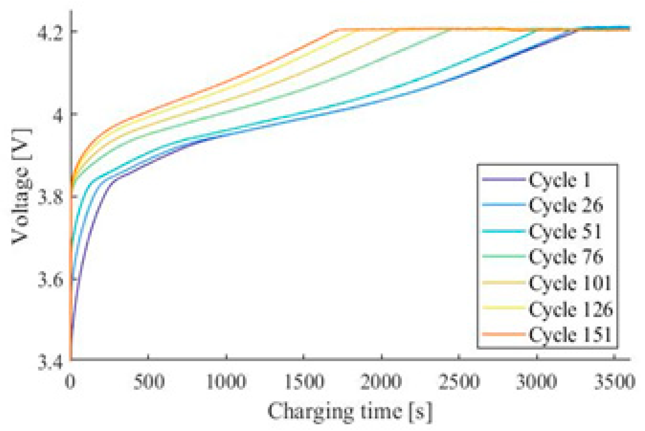
Figure 1. Charging curves at different cycles for battery 5.
Energies 16 04423 g001
Figure 2. PCT values calculated considering the voltage limits of 3.7 V to 4.1 V, with a voltage range of 0.1 V, as a function of number of cycles, for battery 5.
Energies 16 04423 g002
Figure 3. SoH estimation of each battery achieved using a model based on MLR and trained on the other two batteries.
Energies 16 04423 g003
Figure 4. SoH estimation of each battery achieved using a model based on SVR and trained on the other two batteries.
Energies 16 04423 g004
Figure 5. SoH estimation of each battery achieved using a model based on RF and trained on the other two batteries.
Energies 16 04423 g005
Figure 6. PCT for voltage range 3.9–3.95 V for all three batteries.
Energies 16 04423 g006
Table 1. Hyperparameter values tuned for the implemented SVR model.
HyperparameterValue
1Box constraint0.1989
2Kernel scale11.55
3Epsilon0.030
4Kernel functionLinear
Table 2. Three-fold CV results for a voltage range of 0.1 V.
Feature SetVoltage RangeNumber of Features Mean   Validation   R 2
Linear RegressionSecond-Degree Polynomial RegressionThird-Degree Polynomial RegressionSVRRandom Forest
A13.7–3.8 V10.5380.5950.6310.6130.660
A23.8–3.9 V10.9180.9160.9210.9390.902
A33.9–4 V10.9470.9270.9300.9630.904
A44–4.1 V10.5540.535/0.7590.743
A53.7–3.9 V20.9010.8970.8940.9170.838
A63.8–4 V20.9450.9390.9460.9710.909
A73.9–4.1 V20.9420.8350.6520.9610.877
Table 3. Three-fold CV results for a voltage range of 0.05 V.
Feature SetVoltage RangeNumber of Features Mean   Validation   R 2
Linear RegressionSecond-Degree Polynomial RegressionThird-Degree Polynomial RegressionSVRRandom Forest
B13.8–3.85 V10.7810.8960.8970.8100.878
B23.85–3.9 V10.9390.9000.9470.9470.908
B33.9–3.95 V10.9370.9180.9160.9490.896
B43.95–4 V10.8950.9000.8800.9380.898
B53.8–3.9 V20.9310.9090.9280.9410.901
B63.85–3.95 V20.9340.9280.9360.9470.909
B73.9–4 V20.9500.9120.9220.9680.903
B83.75–3.9 V30.9150.8850.8930.9350.883
B93.8–3.95 V30.8990.9110.8950.9480.905
B103.85–4 V30.9430.9380.8960.9640.910
B113.9–4.05 V30.9390.7560.8840.9620.898
B123.8–4 V40.9360.9220.8850.9660.907
B133.85–4.05 V40.9310.864/0.9580.911
B143.9–4.1 V40.9340.775/0.9720.892
Disclaimer/Publisher’s Note: The statements, opinions and data contained in all publications are solely those of the individual author(s) and contributor(s) and not of MDPI and/or the editor(s). MDPI and/or the editor(s) disclaim responsibility for any injury to people or property resulting from any ideas, methods, instructions or products referred to in the content.