Classification of Anomaly Patterns in Integrated Energy Systems Based on Conditional Variational Autoencoder and Attention Mechanism

Abstract

By studying the classification of anomaly patterns in integrated energy systems, a deeper understanding of their operational status can be gained, leading to improved reliability and efficiency. This can ultimately result in reduced energy consumption and carbon emissions, contributing to sustainability efforts. This paper proposes a classification method that employs a conditional variational autoencoder and attention mechanism for deep clustering to identify anomaly patterns and distinguish between normal and anomaly datasets. The proposed model effectively addresses the issue of detecting anomalous periods in traditional anomaly detection methods. To account for the periodicity and coupling relationships of different loads, the model integrates sliding windows and attention mechanisms to improve the accuracy of detecting anomaly patterns. Firstly, during the encoder stage, a spatial attention mechanism is incorporated to extract features at each time step of the model input. Secondly, during the decoder stage, a temporal attention mechanism is introduced to perform feature extraction among the multiple time-step hidden layer states of the model input. The proposed method is applied to a typical integrated energy system and compared with existing methods. The experimental results demonstrate the effectiveness of the proposed method in accurately classifying the normal and anomaly patterns of integrated energy systems due to the internal clustering evaluation index.

1. Introduction

As shown in Figure 1, integrated energy systems integrate various forms of energy supply, conversion, and storage devices, enabling the coupling of different types of energy in source, network, load, and storage [1]. Comprising several energy subsystems, including power, thermal, gas, and energy storage systems, the integrated energy system enables the interaction and exchange of energy, information, and services through various technologies and equipment.

The power system, serving as the core of the integrated energy system, encompasses the generation, transmission, distribution, and consumption of electricity. The thermal system involves heating and cooling processes, which are coupled with the power system to realize various forms of energy complementarity, such as combined heat and power (CHP) and district heating. The gas system mainly consists of natural gas and liquefied petroleum gas supply and storage facilities, which can be coordinated with the power and thermal systems for optimal multi-energy utilization. The energy storage system, comprising various forms of storage technologies such as batteries, supercapacitors, and compressed air energy storage, can alleviate energy fluctuations and improve energy utilization efficiency.

The integration and interaction of these subsystems are achieved through diverse technologies and equipment, forming an efficient energy ecosystem. For example, the power and thermal systems can coordinate with each other to realize energy complementarity and optimize energy utilization through various forms of CHP and district heating. Meanwhile, the energy storage system can smooth out energy fluctuations, thus enhancing energy utilization efficiency.

This integration is a significant manifestation of new-generation energy systems. Accurate short-term load forecasting serves as the foundation for the effective operation and dispatch of integrated energy systems, and the importance of its accuracy is self-evident [2].

The adoption of accurate prediction methods can enhance the stability and reliability of integrated energy systems (IESs). In recent years, load prediction methods, particularly those based on deep learning, have gained widespread use due to their ability to handle nonlinear data and achieve high prediction accuracy [3]. Over the years, numerous studies have investigated different methods for electrical load forecasting. These approaches range from fuzzy theory [4] and support vector machines [5] to gray models [6], random forests [7], autoregressive difference sliding average models [8], neural networks, and combinatorial models [9].

Compared to a single energy system, an integrated energy system couples different types of energy sources to each other through energy conversion equipment, resulting in varying coupling relationships between different types of loads. Therefore, in the load forecasting of integrated energy systems, it is imperative to consider the coupling relationship between different types of loads. The consideration of such coupling relationships is essential in making accurate load forecasts for integrated energy systems.

Multiple scholars have incorporated multi-task learning (MTL) into IES multiple-load forecasting. In the literature, MTL and deep belief networks (DBNs) have been utilized to develop short-term electric, thermal, and gas load forecasting models [10]. Additionally, the weight-sharing mechanism in MTL and least squares support vector machine (LSSVM) has been employed to predict electric, heat, cooling, and gas loads in IESs [11]. In the literature, MTL-LSTM based on IES multiple-load forecasting has been proposed [12]. Additionally, an IES multiple-load ultra-short-term forecasting model based on long-term and short-term time series networks has been proposed [13]. This model considers the uncertainty, periodicity, and interdependence of electric, cooling, and heating loads. Furthermore, it significantly reduces the training cost while maintaining high prediction accuracy.

To date, most studies have focused on comprehensive energy load forecasting in conventional patterns, which do not meet the actual system operation requirements with diverse patterns and variable operating conditions. Existing work has failed to fully exploit and utilize anomaly scenarios. Therefore, it is critical to select a suitable method for anomaly patterns classification.

Anomaly detection involves identifying outliers in a dataset that do not conform to the expected pattern, which can be seen as a classification problem for unbalanced data [14]. The essence of anomaly detection lies in constructing a suitable model to automatically learn the deep features of the data and obtain the decision boundary between normal and abnormal data points, thus effectively distinguishing normal and abnormal samples.

Time series data comprise a sequence of metric data collected at regular time intervals. Examples of such data include network traffic changes, quantitative transactions in banks, and environmental monitoring in industrial Internet of Things. The data analyzed in this paper focus on the integrated energy system and fall under the category of time series data.

Traditional statistical methods, such as moving difference autoregression, can decompose and smooth time series, while anomaly detection can be applied to non-stationary time series with clear seasonality and trend [15]. However, these methods may not be able to capture high-dimensional or nonlinear relationships due to the curse of dimensionality, and may struggle with ambiguous classification of data into normal and anomalous. Classification techniques such as support vector machines [16], decision trees [17], and random forests, and regression algorithms such as XGBoost [18], can solve these issues by better fitting nonlinear or high-dimensional data, reducing overfitting, and improving the model’s generalization ability. However, traditional anomaly detection methods for key performance indicators often do not fully incorporate contextual information of the time series data, which can make it difficult to capture the relationship between anomalies and the full-text information.

Attention mechanisms have been widely used in various fields of machine learning and artificial intelligence, including natural language processing, image recognition, speech recognition, and recommendation systems. In the context of IESs, there have been several recent studies that have utilized an attention mechanism to improve the performance of algorithms.

Yue et al. proposed a multi-task learning approach based on a gated recurrent unit and attention mechanism for multi-load prediction in integrated energy systems [19]. An attention mechanism was used to extract important features from the shared layer for different sub-tasks. They showed that the attention mechanism helped the model to focus on the most informative features and improve the detection accuracy.

Another relevant study is “Short-term Prediction of Urban Energy Multi-load based on MRMR and Dual Attention Mechanism” by Bai et al., where the authors proposed a novel short-term prediction method for the multi-load of urban energy systems by combining the minimum redundancy maximum relevance (MRMR) analysis method with a dual attention mechanism and a sequence-to-sequence (Seq2Seq) neural network. Based on the Seq2Seq model, the dual attention mechanism was integrated into the long-short term memory network, enhancing the algorithm’s ability to learn spatiotemporal features of feature sequences. The attention mechanism was used to highlight the most relevant information and improve the accuracy of anomaly detection [20].

Furthermore, attention mechanisms have also been used in other domains related to anomaly detection. For instance, in the paper “A Novel Deep Policy Gradient Action Quantization for Trusted Collaborative Computation in Intelligent Vehicle Networks” by Chen et al., the authors proposed a trusted deep reinforcement learning (DRL) cybersecurity approach for computation offloading to evaluate the safety and reliability performance in IoT edge networks, including our intelligent system model and a Deep Policy Gradient Action Quantization (DPGAQ) scheme. By introducing a reputation record table and designing a highly decisive communication trusted computing mode, they can accurately predict the untrusted selfish attack of vehicles in the task offloading of the Internet of Things [21].

Overall, these studies demonstrate the effectiveness of the attention mechanism in improving the performance of machine learning models in the domain of IESs, including forecasting. However, further research is still required in the field of classification problems for IESs.

The Classification of Anomaly Patterns in Integrated Energy Systems Based on Conditional Variational Autoencoder and Attention Mechanism provides an innovative advance in the domain of anomaly detection in integrated energy systems. By incorporating a conditional variational autoencoder and an attention mechanism, the model can effectively extract and analyze the complex relationships between different energy sources, enabling accurate identification and classification of anomalous patterns. This approach represents a significant improvement over traditional anomaly detection methods, which often struggle to detect time period anomalies and do not fully consider the complex interactions between different energy systems. Thus, this study provides a valuable contribution to the field of integrated energy system monitoring and management, with the potential to improve energy efficiency and reduce system downtime. The experimental results demonstrate the effectiveness of the proposed method in accurately classifying the normal and anomaly patterns of integrated energy systems. The main contributions of this paper are described as follows:

• Definition of the manifestations of anomaly patterns in the operation scenarios of integrated energy systems;
• The paper proposes a novel approach to anomaly detection in integrated energy systems, specifically by using a conditional variational autoencoder (CVAE) and attention mechanism. The use of CVAE allows for the modeling of conditional distributions, which is important in the context of integrated energy systems where anomalies may occur in specific conditions or contexts. The attention mechanism is used to enhance feature extraction and capture complex dependencies between the multivariate load and other input features in the system.
• The paper demonstrates the effectiveness of the proposed approach through experiments on real-world data, showing improved performance compared to traditional methods such as K-means and autoencoder-based approaches in the internal clustering evaluation index.

2. Conditional Variational Autoencoder Based on Attention Mechanism (CVAE-A) Mode

2.1. Definition of Anomaly Patterns in Integrated Energy Systems

Multiple-load forecasting involves anomaly patterns that are rare but can have a significant impact on load forecasts. These patterns may arise from unexpected events, natural disasters, technical failures, or policy changes. Anomaly patterns in load forecasting can cause the load to deviate from expected values, thereby affecting energy supply and consumption.

Anomaly patterns can include a variety of scenarios, as follows:

• Emergencies such as severe weather, power outages, and natural disasters, can lead to rapid increases or decreases in load;
• Policy changes such as adjustments in government policies, can also have an impact on energy use, which may affect changes in load;
• Sudden demand such as during holidays or special events, can lead to rapid increases or decreases in load;
• New technologies: The introduction of new technologies can have an impact on energy consumption, which may also result in changes in load.

For the different anomaly pattern scenarios mentioned above, the anomaly patterns in the integrated energy system have the following characteristics, as shown in

Table 1. Features of the anomaly pattern.

Features	Causes
Sharp changes	These patterns often result in abrupt changes in load, such as a sudden drop in load due to natural disasters or technical failures, or a rapid increase in load due to a surge in electricity demand during special events.
Long duration	Anomaly patterns may persist for a period of time. For example, a prolonged increase in electricity consumption for air conditioning during consecutive hot weather days may result in a continuous rise in load.
Non-periodic	Anomaly patterns are usually non-periodic, i.e., their timing and periodicity are irregular and difficult to predict with conventional periodic models.
High volatility	The volatility of load usually increases in the anomaly pattern. The variation in load values becomes larger, which may result in an increase in forecast errors.

.

The proposed method in this paper distinguishes between normal and anomaly patterns by utilizing deep clustering. Anomaly patterns are identified by the presence of large clustering losses between the load data and the clustering center. Thus, the clustering loss can be used as an indicator to detect whether a load change at a specific time is indicative of an anomaly pattern.

2.2. Data Preparation

In order to enhance the model’s ability to classify load data, it is necessary to consider various features that can affect load classification, such as historical electrical, cooling, and thermal load data, calendar data, and other relevant information. In this study, we use the IES [22] of Arizona State University Tempe campus, USA, as an example, and the dataset from 1 January 2020 to 31 December 2020 is used for analysis. The original dataset is divided into three types of loads: electric, cooling, and heating, with a sampling period of 1 h. To ensure the maximum expressiveness of the model, we take into account all relevant features that may influence load classification.

Considering the time series characteristics of multiple loads, when classifying anomaly patterns of multiple loads, not only are the forecasted historical loads considered, including cooling, heat, and electric load, but also the weather factors, such as temperature and humidity at the current moment.

The original time series plot of electricity, cooling, and heating loads in May is shown in Figure 2. The raw data are sampled hourly, with a total of 8784 time steps. The x-axis range in this figure is from 2905 to 3648, corresponding to the date range from 1 May at 0:00 to 31 May at 23:00.

2.2.1. Autocorrelation Analysis

To test whether there is a cyclical relationship between the loads, autocorrelation graphs for selected data in each load are plotted in Figure 2. This has important implications for the selection of the number of sliding windows and the application of the temporal attention mechanism.

The autocorrelation coefficient is the degree of correlation between the same event in different periods. It can also be understood as the correlation between the past and present of the same individual. The equation for the autocorrelation coefficient is shown in Equation (1):

$$\rho \left(t,s\right)=\frac{E\left(x_t-\mu \right)\left(x_s-\mu \right)}{\sqrt{D{x}_t{x}_s}}$$

(1)

where E is the expectation, D is the variance, $\mu$ is the mean value, and $x_t$, $x_s$ represent the load series signal at moment t.

Figure 3 clearly shows a short-term repetitive pattern with a period of days and an ultra-long-term repetitive pattern with a period of weeks. This is significant for the classification of multiple-load anomaly patterns. As previously mentioned, anomaly patterns lack periodicity, but the temporal attention mechanism can aid in learning the periodic relationships within the dataset. This enables the detection of anomaly patterns present in the dataset.

2.2.2. Data Pre-Processing

In order to effectively utilize the electrical, cooling, and thermal load data, which have different units and value ranges, normalization is necessary. The load data in this study are scaled to the range of [0, 1] using min-max standardization. This transformation results in dimensionless values, enabling the comparison and weighting of different data sequences. Additionally, normalization prevents gradient explosion during the training process, leading to more efficient network training. Furthermore, to handle individual data abnormalities during acquisition, the mean correction method is used to deal with outliers and ensure the high quality of the dataset.

$$\tilde{x}\left(i\right)=\frac{x\left(i\right)-x_{min}}{x_{max}-x_{min}}$$

(2)

$x\left(i\right)$ is the input feature sequence, $\tilde{x}\left(i\right)$ is the normalized sequence, and $x_{max}$ and $x_{min}$ are the minimum and maximum values of the sample data, respectively. After the normalization process, the values of the data are within [0, 1].

2.2.3. Analysis of Multiple-Load Related Factors

In an IES, multiple loads are interdependent, and when one load is in the anomaly pattern, it is highly likely that other loads are also in the anomaly pattern. Therefore, the data of other loads, such as cooling and heating loads, can be utilized to identify the pattern to which they belong. To improve the accuracy of anomaly pattern judgment, different loads are assigned different weights based on the input data. By taking into account the interdependence of loads and their correlations, the proposed method uses deep clustering to distinguish between normal and anomaly patterns, where the latter is characterized by a large clustering loss between the load data and the clustering center. This clustering loss can be utilized to determine if a load change at a certain time is an anomaly pattern.

In this study, Spearman’s rank correlation coefficient is employed to examine the correlation between electric, cooling, and heating loads.

As can be seen from Figure 4, there is an extremely strong correlation between electric, cooling, and heating loads, proving the superiority of using multiple loads for anomaly pattern classification.

2.3. Conditional Variational Autoencoder (CVAE)

As a specific type of encoder model, a variational autoencoder (VAE) is typically employed for data generation. By projecting the input observed variables into a low-dimensional feature space, VAE aims to ensure minimal reconstruction error and to have their feature distributions as closely aligned as possible with a pre-assumed prior distribution. Usually, the prior distribution is set to be the standard normal distribution N (0,1). As a result, the distribution of the data generated from the prior distribution can be approximated to be the same as the distribution of the real observed data. However, the simple assumption of the prior distribution can result in poor performance of traditional VAE for modeling complex distributions.

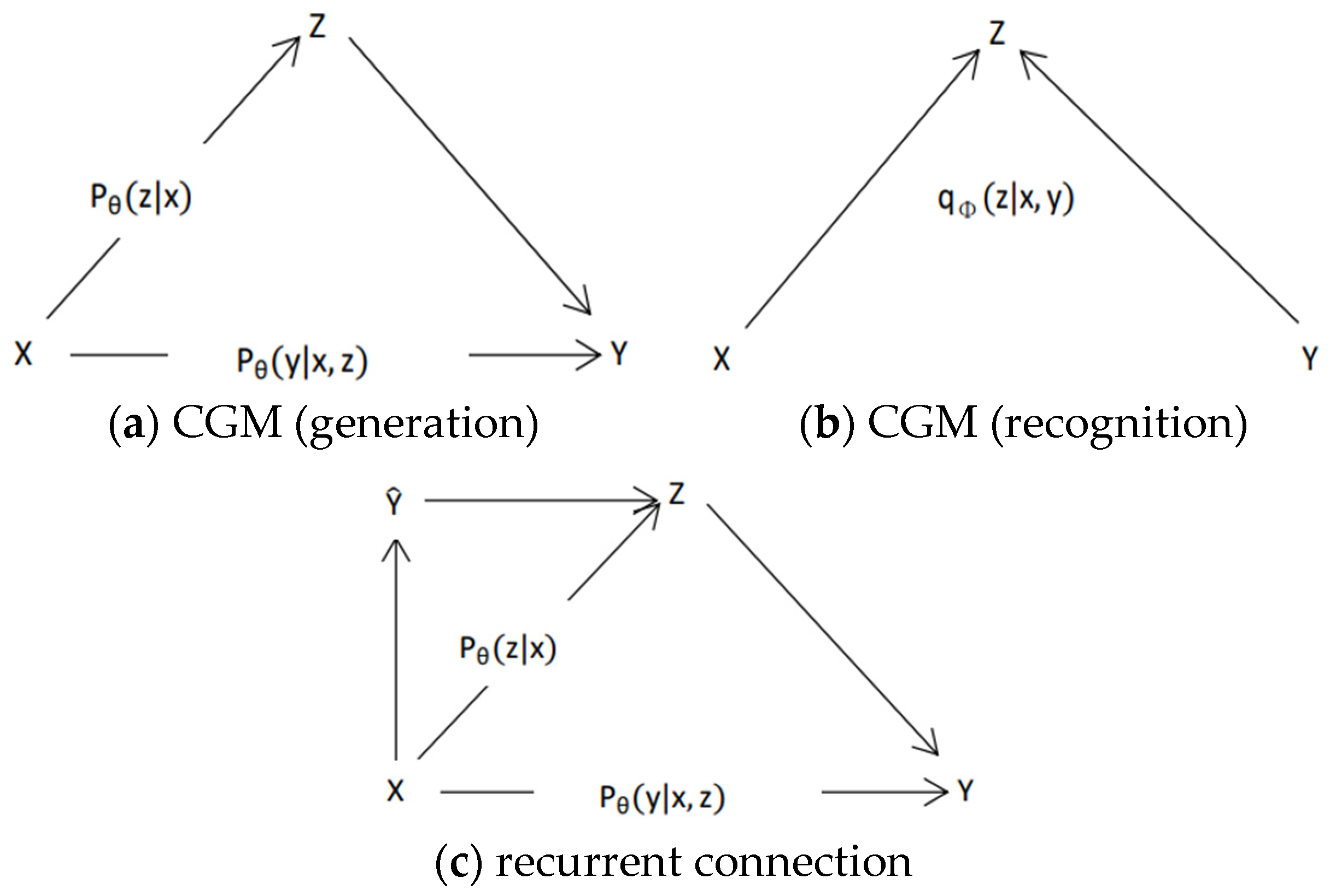
To capture more complex distributions, CVAE includes conditional constraints on the traditional VAE model to determine the prior distribution based on input conditions. Like VAE, CVAE also involves two processes: generation and recognition. The CVAE model is comprised of three components: a prior network, a recognition network, and a generation network, as depicted in Figure 5 [23].

The identification network determines the posterior distribution $q_{\varphi }(z|x,c)$ in the identification process, where the inputs are the observed variable x and the condition c. In the generative process, the prior distribution $p_{\theta }\left(z,c\right)$ is determined by the input c of the prior network. The generative network $p_{\theta }(x|z,c)$ uses the latent variable z and condition c as inputs to generate the observed variables. If CVAE is used for data generation, the latent variable z is generated according to the conditional distribution $p_{\theta }\left(z,c\right)$. If CVAE is used for data reconstruction, the latent variable z is sampled from the distribution $q_{\varphi }(z|x,c)$. The computational framework of CVAE is shown in Figure 6. The dashed line in the figure indicates the loss term of the objective function.

The training objective of the CVAE model is to maximize the conditional log-likelihood of:

$$\max \log p(X|C)=\max {\sum }_{\mathrm{i}=1}^{\mathrm{N}}\log p(x_i|c_i)$$

(3)

Given the training sample ($x_i$,$c_i$), the distribution $q_{\varphi }(z|x_i,c_i)$ and $p_{\theta }(x|x_i,c_i)$ the KL scatter between them is:

$$\begin{gathered} D_{KL}[q_{\varphi }(z|x_i,c_i)\left|\right|p_{\theta }(x|x_i,c_i)] \\ =-E_{z~q}\left[\log p_{\theta }\left(x|z,c_i\right)\right]+D_{KL}[\log q_{\varphi }\left(z|x_i,c_i\right)||\log p_{\theta }\left(z|x_i\right)]+\log p_{\theta }(x_i|c_i) \end{gathered}$$

(4)

The posterior distribution $q_{\varphi }(z|x_i,c_i)$ is a variational approximation of the true distribution $p_{\theta }(x|x_i,c_i)$. When the posterior distribution is close enough to the true distribution, the KL scatter is close to 0. When the posterior distribution is sufficiently close to the true distribution, the KL scatter is close to 0. Due to the non-negativity of the KL scatter, the variational low bound of log p(x|c) is used as the optimization objective function of the model:

$$\mathrm{L}\left(\theta ,\varphi ;x_i,c_i\right)=\log p_{\theta }(x_i|c_i) -\mathit{KL} \left[q_{\varphi }\left(z|x_i,c_i\right)\right||p_{\theta }\left(z|x_i,c_i\right)$$

(5)

The training objective of CVAE is to maximize $\mathrm{L}\left(\theta ,\varphi ;x_i,c_i\right)$:

$$\mathrm{L}\left(\theta ,\varphi ;x_i,c_i\right)=E_{z~q}[\log p_{\theta }\left(x_i|z,c_i\right)] - D_{KL}[q_{\varphi }\left(z|x_i,c_i\right)\left|\right|p_{\theta }\left(z|c_i\right)]$$

(6)

2.4. Conditional Variational Autoencoder Based on the Attention Mechanism (CVAE-A)

This paper presents a classification of anomaly patterns in integrated energy systems based on the conditional variational autoencoder and attention mechanism. The conditional variational autoencoder is a probabilistic graphical model that combines variational inference with deep learning, in which using reconstruction probabilities as anomaly scores is more principled and objective than reconstruction errors.

Furthermore, this method explicitly explores the potential variations and diversities inherent in the training samples by introducing an attention mechanism that acquires dynamic weights for each variable. By fusing the variation factors found in the samples with the final latent variables, the attention mechanism enhances the model’s classification ability.

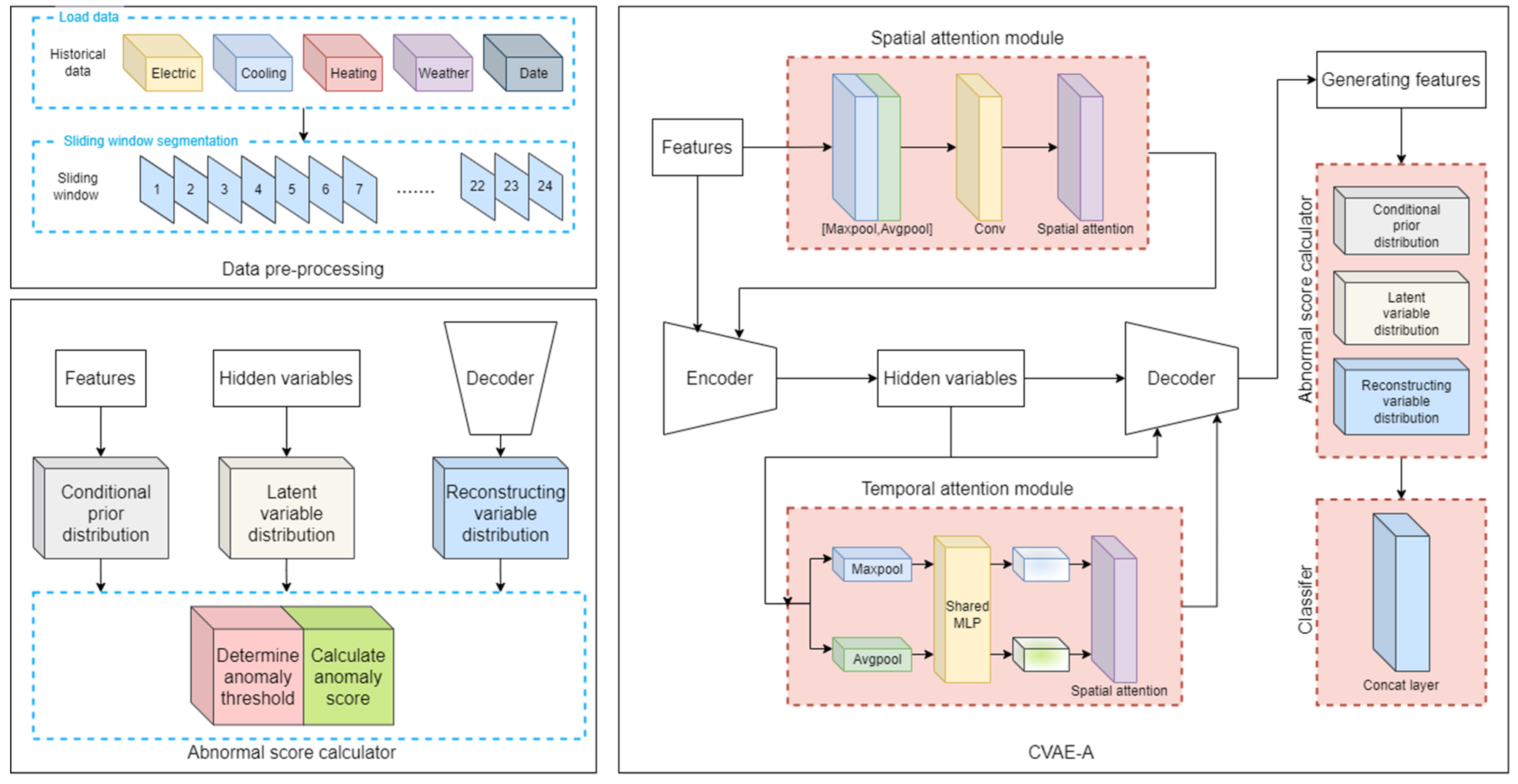
This paper presents the framework of the CVAE-A model, as illustrated in Figure 7, which consists of three steps.

Firstly, a spatial attention mechanism is introduced in the encoder stage to extract features in each time step of the model input. The feature vector sequence with the highest value at that time step is analyzed.

Secondly, a temporal attention mechanism is introduced in the decoder stage to weight and sum the intermediate latent variables, which yields the final latent variables.

Finally, the final latent variables are decoded. By extracting and integrating the rich feature information of the original samples, the proposed method enhances the accuracy of the model’s classification.

2.4.1. Attention Mechanism

The traditional attention mechanism is effective in filtering and extracting information within the model. It can address the issues of inefficient convergence and information loss that arise due to unreasonable input length and order in general RNNs. Therefore, it performs well in the mode classification of general electric loads. However, in an integrated energy system, there are multiple energy sources operating simultaneously, such as cooling, heating, and electricity, and there are complex coupling relationships between them. The data input includes the information of many features that are difficult to intuitively describe but are significantly related. Therefore, a dual attention (DA) mechanism is needed to enhance feature extraction.

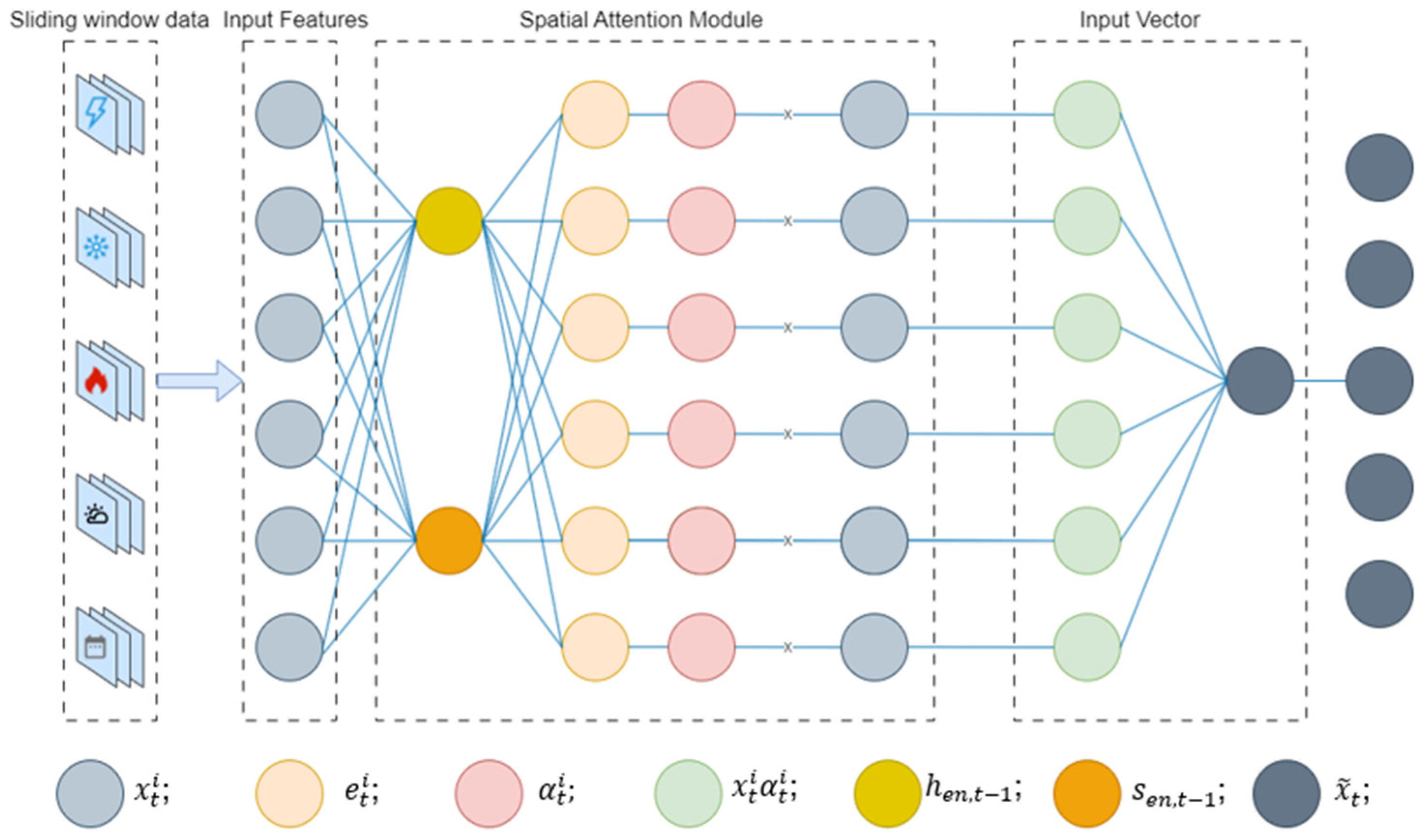
Under the DA mechanism, the encoder and decoder each contain an attention layer that can find correlations between feature representations and target sequences in space and time, respectively. They assign different weights to different information to more accurately identify anomaly patterns. The encoder attention mechanism and the decoder attention mechanism are illustrated in Figure 8 and Figure 9, respectively.

2.4.2. Encoder (Spatial Attention Module)

As shown in Figure 7, during the encoder stage, a spatial attention mechanism is incorporated to extract features at each time step of the model input. This mechanism analyzes the higher value set of all feature vector sequences at each time step and assigns higher weights to them, thus learning the spatial dependencies between the multivariate load and other input features.

The original input sequence is X = [$x^1$, $x^2$, …, $x^n$] consisting of a total of n input features, where $x^{\mathrm{i}}$ = [$x_1^i$, $x_2^i$, …, $x_T^i$] represents the i-th feature sequence with step size T. $x_T^i$ is the input sequence at moment t in the i-th feature sequence, i = 1, 2, …, n, and t = 1, 2,…, T. Thus, the input sequence at the same step is $x_t$ = [$x_t^1$, $x_t^2$, …, $x_t^n$].

The state $h_{en,t}$ of the hidden layer in the encoder stage can be expressed as:

$$h_{en,t}=f_{en}(h_{en,t-1}, x_t)$$

(7)

Then, each feature weight ${\alpha }_t^i$ is calculated based on $h_{en,t-1}$ of the previous time and the neuron state $s_{en,t-1}$ of the encoder.

$${\alpha }_t^i=\frac{\exp \left(e_t^i\right)}{{\sum }_{k=1}^n\exp \left(e_t^k\right)}$$

(8)

$$e_t^i=v_e^{\prime }\tan \mathrm{h} (W_e\left[h_{en,t-1},s_{en,t-1} \right]+U_e{x}^i)$$

(9)

where $v_e^{\prime }$,$W_e$, and $U_e$ represent the parameters to be learned; $e_t^i$ is the weight of the ith feature sequence at time t; ${\alpha }_t^i$ is the result of normalizing the weight of the ith feature sequence at time t.

By using the attention mechanism, the model combines information from the hidden layers for each dimension feature with specific weights to obtain a new input sequence, ${\tilde{x}}_t$:

$${\tilde{x}}_t=\left[x_t^1{\alpha }_t^1,x_t^2{\alpha }_t^2, \dots ,x_t^n{\alpha }_t^n\right]$$

(10)

The hidden layer state $h_{en,t}$ is recalculated:

$$h_{en,t}=f_{en}(h_{en,t-1}, {\tilde{x}}_t)$$

(11)

2.4.3. Decoder (Temporal Attention Module)

As shown in Figure 8, the temporal attention mechanism is introduced during the decoder stage to perform feature extraction among the multiple time-step hidden layer states of the model input. The mechanism analyzes the hidden layer states of different time steps and assigns higher weights to the ones with higher values.

The decoder hidden layer state $h_{de,t-1}$ and the neuron state $s_{de,t-1}$ are weighted and averaged over the encoder hidden layer state $h_{en,t}$ by using the attention mechanism of the decoder.

First, the weights ${\beta }_t^m$ are calculated based on the encoder’s hidden layer state and the decoder’s neuron state; the hidden layer state is:

$${\beta }_t^m=\frac{\exp \left(l_t^m\right)}{{\sum }_{j=1}^T\exp (l_t^j)}$$

(12)

$$l_t^m=v_d^{\prime }\tan \mathrm{h} \left(W_d\left[h_{de,t-1},s_{de,t-1} \right]+U_d{h}_{en,m}\right)$$

(13)

The semantic vector $c_t$ is obtained after weighting:

$$c_t=\sum _{m=1}^T{\beta }_t^m{h}_{en,m}$$

(14)

where $v_d^{\prime }$,$W_d,\mathrm{and} U_d$ represent the learnable parameters; $l_t^m$ denotes the weight of the hidden layer state $h_{en,m}$ at the encoder step m; and ${\beta }_t^m$ represents the normalized weight.

The hidden layer state $h_{de,t}$ is computed using the updated ${\tilde{y}}_{t-1}$ as follows:

$$h_{de,t}=f_{de}\left(h_{de,t-1}, {\tilde{y}}_{t-1}\right)$$

(15)

2.4.4. Classification Process

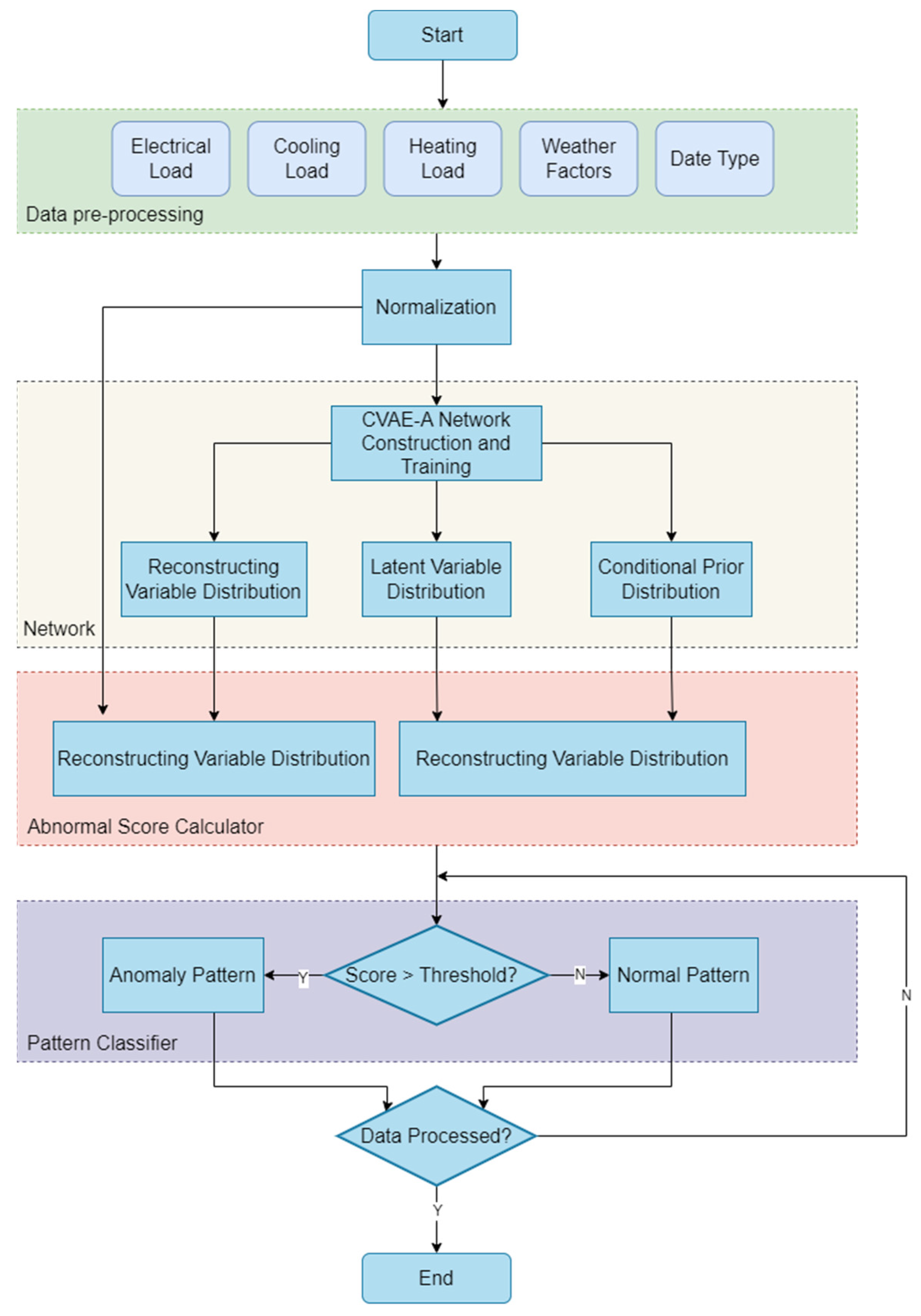
The flowchart of the classification model in this paper is illustrated in Figure 10. The process consists of three main stages: raw data processing, neural network construction, and anomaly score calculation. The neural network construction adopts the classification model of the integrated energy system based on the conditional variational autoencoder and double attention mechanism proposed in this paper. Finally, the final classification results of the normal and abnormal modes of the integrated energy system are obtained.

2.5. Experimental Procedure

The hardware configuration of the experimental platform included an NVIDIA GeForce RTX 2080 8G graphics card and software with the Windows 10 operating system and MATLAB R2022b. Both the generative and recognition models of the CVAE model were designed as three-layer neural networks (i.e., containing only one hidden layer), with Tanh as the hidden layer activation function and a hidden layer dimension of 50. The model is trained using the Adam gradient update strategy, and the learning rate is set to ${10}^{-3}$.

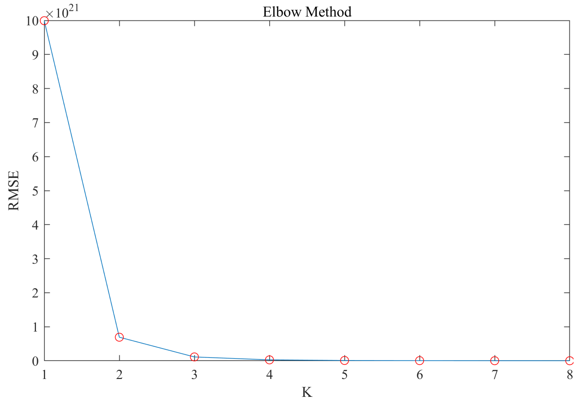
To be more precise, the experiment used the load data of an integrated energy system from 1 January 2020 to 31 December 2020. To calculate the similarity between any two days’ load data, the minimum cumulative distance method was used. Then, the elbow criterion was applied to determine the number of clustering centers, and the K-means method was used to cluster the load data. The clustering error of the load data on a certain day was used to determine whether the load change on that day belonged to an anomaly pattern.

Subsequently, the load data from 1 April 2021 to 31 May 2021 were divided into sliding windows of size 24. CVAE-A was used to detect anomalous data based on whether the data in the sliding windows belonged to anomaly patterns. The proposed method’s accuracy in predicting extreme patterns was evaluated by comparing it with that of other anomalous pattern detection methods, such as statistical, K-means, autoencoder, variational autoencoder, conditional variational autoencoder, and isolated forest. The parameters for each comparison algorithm were selected and set as shown in

Table 2. Selection of parameters.

Algorithm	Parameter Values
Statistical Method	Confidence level is 95%;
K-means	The number of clusters is 2;
CVAE	Both the generative and recognition models of the CVAE model are designed as three-layer neural networks (i.e., containing only one hidden layer), with Tanh as the hidden layer activation function and a hidden layer dimension of 50. The model is trained using the Adam gradient update strategy, and the learning rate is set to 10−3.
Isolated Forest	The number of random trees is 100.
CVAE-A	Both the generative and recognition models of the CVAE-A model are designed as three-layer neural networks (i.e., containing only one hidden layer), with Tanh as the hidden layer activation function and a hidden layer dimension of 50. The model is trained using the Adam gradient update strategy, and the learning rate is set to 10−3.

.

By conducting these experiments, we aimed to demonstrate the effectiveness of the proposed method in detecting extreme patterns in load data. This can contribute to improving the reliability and efficiency of the system, reducing energy consumption and carbon emissions, and promoting the application and development of deep learning and anomaly pattern recognition in the field of integrated energy systems.

3. Results

In this study, clustering is employed to distinguish between normal and anomaly load patterns. Before clustering the load data, the optimal number of cluster centers (i.e., classifications) K is determined using the elbow rule. The elbow rule works by measuring the minimum cumulative distance between load data and the cluster center to determine the degree of distortion of the data. A curve representing all minimum cumulative distances is plotted, and the optimal k value is determined where the curve decreases the most.

Figure 11 illustrates the distortion curves for different numbers of cluster centers. As shown in the figure, the degree of distortion decreases faster when k = 1 and slower when k > 2. Therefore, the number of clustering centers, k, is chosen to be 2.

For this section, six anomaly detection methods were selected to be compared with the methods presented in this paper to evaluate the effectiveness of the proposed methods. The load data anomalies in the conventional mode are mainly manifested by missing data values, including single or continuous data; the load data anomalies in the anomaly patterns are mainly manifested by sudden changes in data values and abnormal data in short time periods.

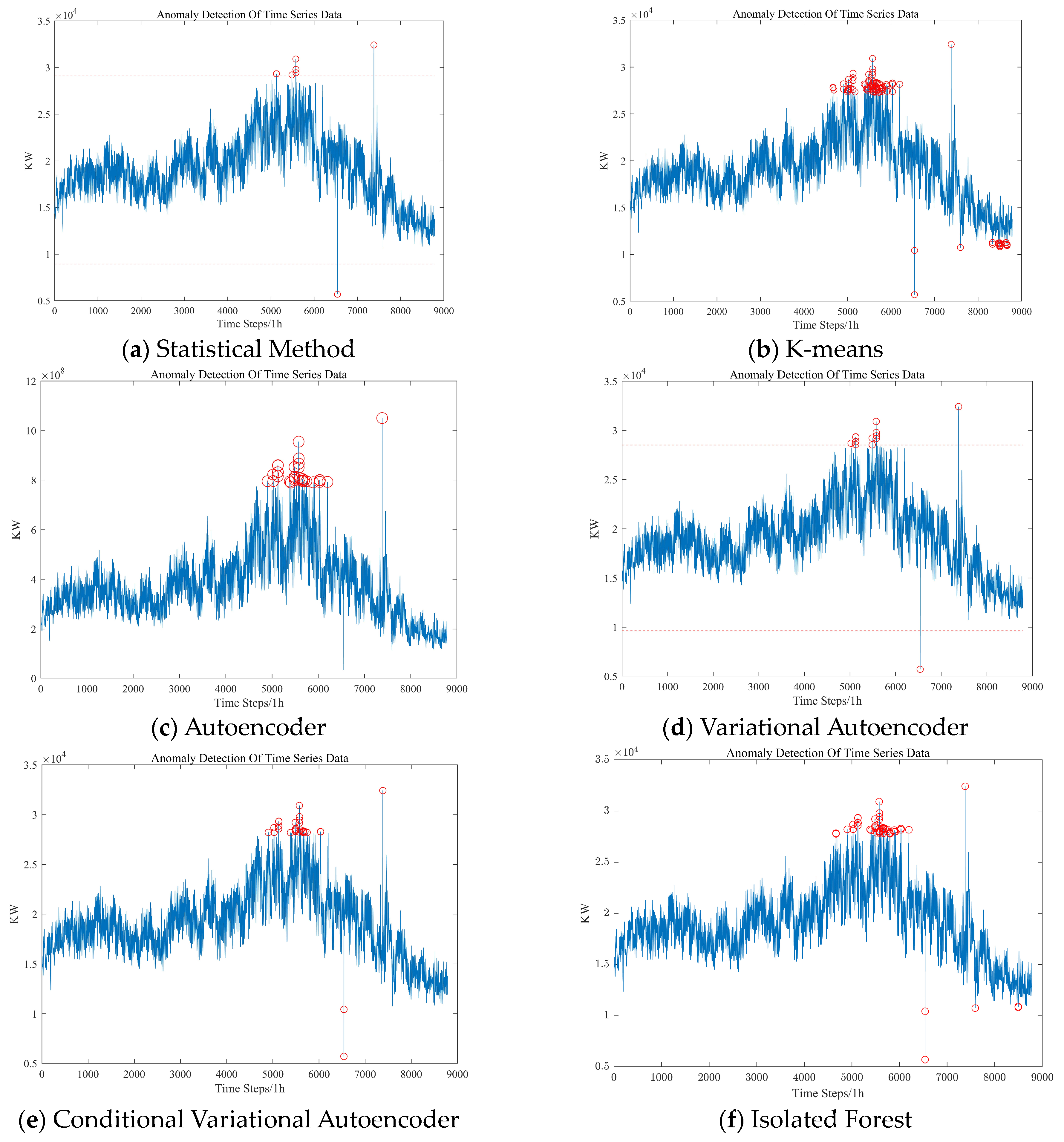
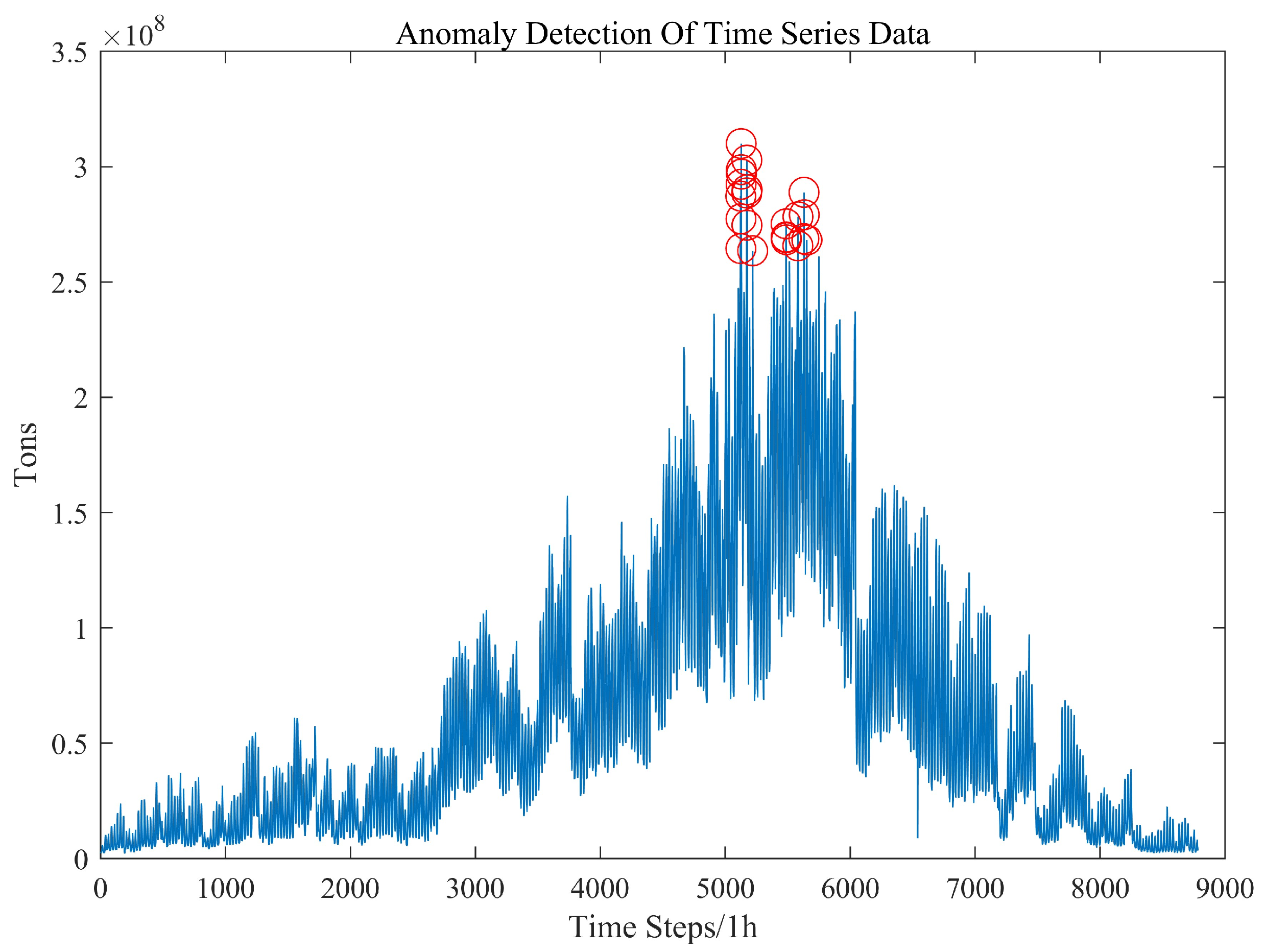
Figure 12 shows the labeling of abnormal electric load data by different methods.

As shown in Figure 12a,d, the red circle represents the anomaly time point, while the red dot line represents the threshold for determining anomaly time points. If it exceeds the threshold, it is considered an anomalous time point.

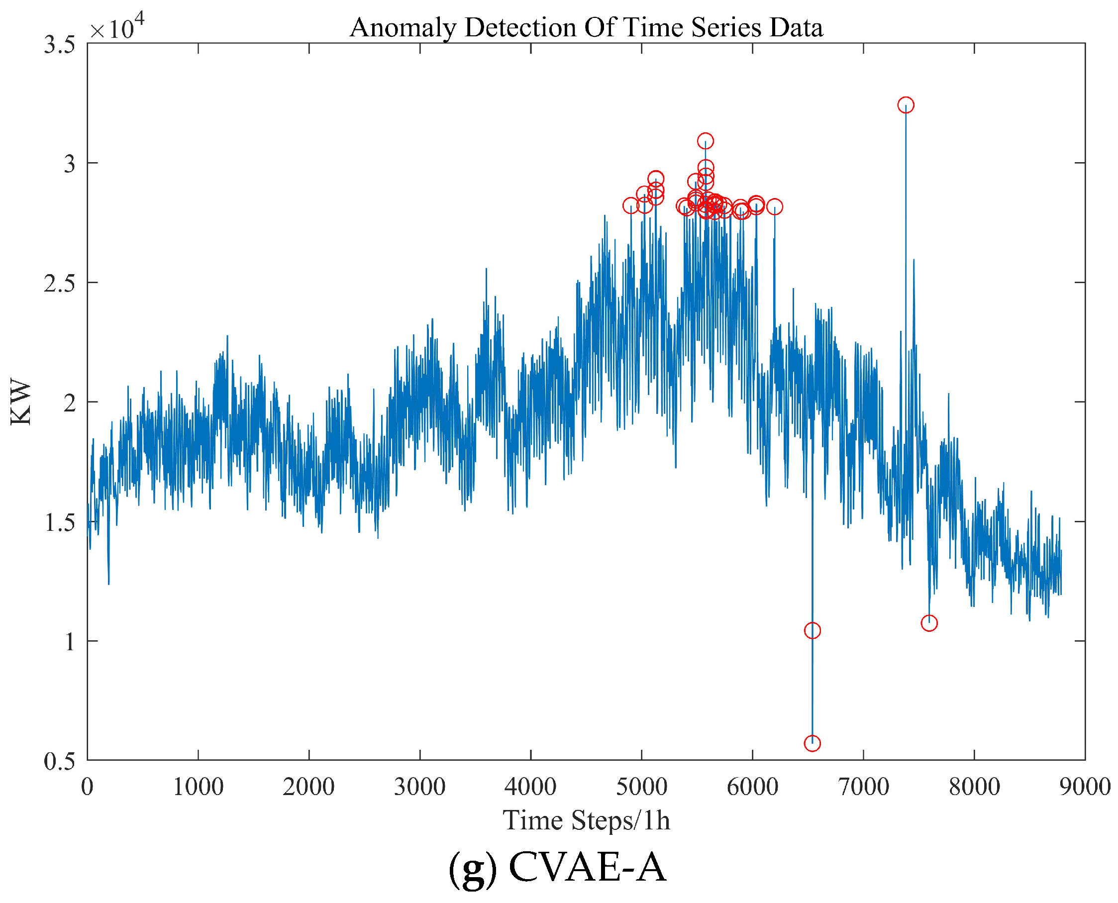
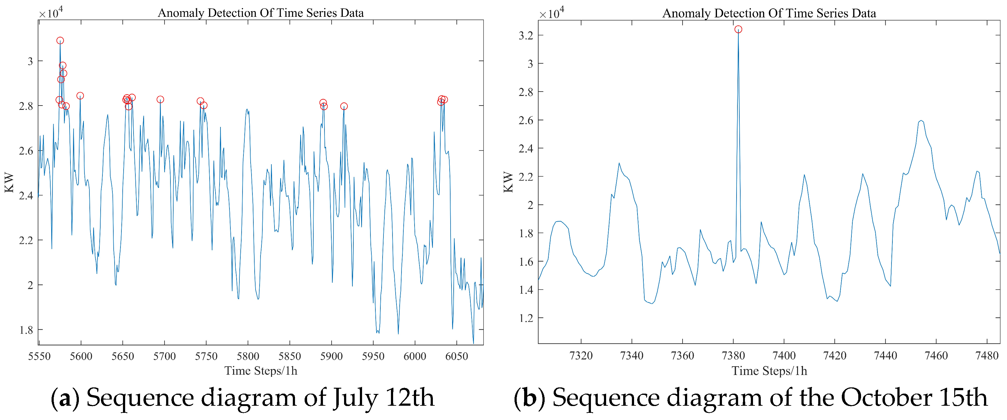
As shown in Figure 12g, a total of 11 days of load variation were selected as anomaly patterns, out of which 5 days were chosen for analysis. Among these anomaly patterns, load variations on 12 July and 15 October were considered anomalies due to missing data.

As shown in Figure 13, since the load data for the two consecutive days following 12 July also belong to the anomaly pattern, it can be presumed that the load change on 12 July was an anomaly. However, the load change around 15 October did not show an anomaly pattern, leading to the judgment that the load change on October 15th did not belong to an anomaly.

Combining the load data with other variables, such as the cooling load, number of classrooms, total number of lights, and greenhouse gas emissions on July 12th, July 13th, July 20th, and September 4th, all showed changes that corresponded to the electric load. Thus, it can be concluded that the load changes on the dates mentioned belonged to the anomaly pattern generated by changes in the operating environment of the integrated energy system.

Figure 14 displays the classification results of cooling load anomaly patterns using the CVAE-A model, which integrates anomaly data from electric, cooling, and heating loads to categorize anomaly patterns in the dataset.

The evaluation methods for clustering results can be generally divided into internal evaluation and external evaluation. The external evaluation method refers to the evaluation of the clustering results with the knowledge of the true labels. Internal evaluation is a method that assesses the quality of clustering results based solely on the properties of the samples and the clustering algorithm used, without relying on external information or labels.

Since the object of this paper is an unlabeled dataset, the effectiveness of the proposed method is evaluated by the internal evaluation method. Common internal assessment methods include Silhouette Coefficient, Calinski–Harabasz Score, and Davies–Bouldin Score. Due to the characteristics of the multivariate load dataset, this paper uses both Silhouette Coefficient and DBI evaluation indices.

Figure 15 shows the performance index values of the different methods.

Considering the characteristics of the multiple-load dataset, the SC and DBI evaluation are used to evaluate the performance of the proposed method. A lower DBI value indicates better clustering results, whereas a higher SC value indicates better performance. The experimental results demonstrate that the proposed method outperforms all the comparison methods in terms of accuracy.

As shown in Figure 13, Figure 14 and Figure 15, the proposed method outperforms all the compared methods in terms of accuracy. The main reasons for this are discussed below.

• The traditional method is sensitive to the distribution of abnormal data. However, in the anomaly pattern, the distribution of load data changes, which can lead to misclassification of normal load data of the anomaly pattern as anomalous by the traditional method.
• The traditional method has a good detection effect on load anomalous data in normal mode, such as single or continuous vacancy values. However, it is less effective in detecting continuous data anomalies in short periods. CVAE-A, on the other hand, can better detect data anomalies in short periods.
• Finally, the proposed method not only detects load data anomalies but also avoids misclassification of extreme mode load normal data, making it suitable for the classification of normal and anomaly patterns of integrated energy systems.

4. Conclusions

In the context of achieving the “dual-carbon” goals, building a new power system that relies on new energy sources as the main source is an important prerequisite and inevitable trend to promote the low-carbon transformation and development of modern power systems. Studying the classification of anomaly patterns in integrated energy systems can lead to a better understanding of the system’s operational status, which in turn can improve its reliability and efficiency while also reducing energy consumption and carbon emissions. Improving the classification methods can provide a more detailed description of the anomaly patterns in integrated energy systems, improve the accuracy and robustness of anomaly pattern classification, and provide better reference and decision-making support for system operation and management. Furthermore, this research can promote the application and development of deep learning and anomaly pattern recognition in the field of integrated energy systems, thereby contributing to the promotion of high-quality, efficient development and carbon reduction in integrated energy systems.