Energy Consumption Prediction of Electric City Buses Using Multiple Linear Regression

Abstract

The widespread electrification of public transportation is increasing and is a powerful way to reduce greenhouse gas (GHG) emissions. Using real-world driving data is crucial for vehicle design and efficient fleet operation. Although electric powertrains are significantly superior to conventional combustion engines in many aspects, such as efficiency, dynamics, noise or pollution and maintenance, there are several factors that still hinder the widespread penetration of e-mobility. One of the most critical points is the high costs—especially of battery electric buses (BEB) due to expensive energy storage systems. Uncertainty about energy demand in the target scenario leads to conservative design, inefficient operation and high costs. This paper is based on a real case study in the city of Seville and presents a methodology to support the transformation of public transportation systems. We investigate large real-world fleet measurement data and introduce and analyze a second-stage feature space to finally predict the vehicles’ energy demand using statistical algorithms. Achieving a prediction accuracy of more than 85%, this simple approach is a proper tool for manufacturers and fleet operators to provide tailored mobility solutions and thus affordable and sustainable public transportation.

1. Introduction

Substituting conventional energy sources in the mobility sector is currently one of the most discussed topics related to climate change, reduction in greenhouse gas (GHG) emissions and sustainability worldwide. While in many sectors GHG emissions have been reduced since the 1990s, traffic causes approximately $25\%$ of the European GHG emissions and is still rising [1]. Legal regulations, demand and public awareness for low-emission vehicles have turbocharged the race to electric mobility [2,3]. The efficiency of electric vehicles (EV) surpasses internal combustion engine vehicles (ICV) by far (up to $77\%$) [4] and powertrain electrification brings many other benefits, such as better vehicle dynamics and reduced noise or pollution levels [4,5,6,7]. Thus, the changeover to alternative powertrains plays a crucial role in the continuously growing [8] global transportation sector. However, planning alternative public transportation systems is challenging because of the comparably high costs of BEVs compared to ICVs [9]. Initial investments for battery electric buses (BEB) are almost double compared to diesel [10]. However, studies also show the enormous difference in energy consumption, life cycle CO₂ emissions and life cycle costs of ICV, PHEV or BEV and reveal the high potential of alternative powertrains [5]. Consequently, the first step to efficient vehicle and fleet operation is accurate knowledge of the energy consumption of each route [11]. Nevertheless, existing approaches are limited by the fact that they either use complex physical models, which cannot adequately consider all influencing factors, or they use data-driven techniques that require a large number of driving, mechanical and roadway measurements. Therefore, it seems necessary to explore ways to simplify the problem.

The starting point for this research is the municipal bus company in Seville that plans the replacement of its Diesel powered fleet with a fully electric one, as well as assessing the feasibility of the manufacturer that will supply the vehicles. We were provided with comprehensive data on the fleet operator, along with information about the vehicle by the manufacturer, to predict the energy demand of the electric buses that will soon be serving the routes. Our main contribution and key difference to previous studies lies in the reduced number of physical quantities to be measured: we prove that it is sufficient to know the vehicle speed and additional payload due to passengers on the bus to accurately predict the consumption on the route. This paper introduces a set of explanatory variables that are used by statistical means to predict the vehicle’s energy demand. This research increases understanding and transparency of vehicles’ energy economy and the simplicity of the final implementation will be useful for manufacturers and operators alike to answer questions, such as what capacity the batteries should have, what is the state of charge of the batteries at any given time or what is the best distribution of charging stations along the route.

Therefore, the paper is structured as follows. First, we identify the challenges in this field and review the state of the art in Section 1. Secondly, our materials and methods are explained in Section 2. The experiments and results are presented in Section 3. Finally, in Section 4, we discuss and conclude our paper.

State of the Art

The prediction of energy demand, for EVs and BEBs in particular, has been thoroughly investigated in previous studies. The majority utilize complex physics-based analytical vehicle models, though they vary in focus and objective [12,13,14,15,16,17,18]. The authors in [12] find that the drivetrain efficiency, the auxiliary power demand and the rolling resistance are the most influential factors affecting the energy consumption of BEVs. Another study by De Cauwer et al. [13] combined a vehicle dynamics model with a data-driven approach to detect and quantify correlations between the kinematic parameters and the vehicle’s energy consumption. Commonly used kinematic parameters are extended by additional factors such as travel distance and time or temperature. Wang et al. [15] present an energy consumption model for BEVs considering the effects of road surface-dependent rolling resistance and changing weather conditions. The authors in [16] use a prediction model that consists of a longitudinal dynamics model complemented by measurements from a dynamometer, as well as coastdown tests, to reduce the model’s uncertainty. All these approaches investigate the interrelation of factors of influence and provide valuable insights; however, they incorporate complex equations and require precise modeling of vehicles and components, which are prone to simplifications, and thus, of limited validity due to simulation restrictions. Additionally, the studies focus mainly on passenger vehicles, and scaling to BEBs is not easily possible because of completely different operational behavior and vehicle dynamics.

In recent years, the prediction of energy consumption for heavy-duty vehicles, especially BEBs in urban areas, became a research field of growing interest. As mentioned before, vehicle dynamics, duty cycle and driving conditions of BEBs differ heavily from that of other BEVs, shifting the focus from kinematic relationships to route, schedule and passenger load. Therefore, the authors in [19] review state-of-the-art energy-consumption estimation models for EVs and study BEBs using logistic regression and neural networks on real-world data. Lajunen [20] presented a comprehensive comparison of hybrid and electric buses, discovering that fully electric vehicles such as BEBs are less sensitive to variations in mission profiles than hybrid or diesel buses. In a similar way, the authors in [21] propose a computationally efficient surrogate model derived from an electro-mechanical model of a BEB. After a factor identification process, they found the payload mass, the temperature and the rolling resistance, albeit in different proportions, to be most important. The aforementioned studies buttress the need for energy consumption and prediction models for BEBs, respectively. However, the underlying data they use are mainly based on a single route or vehicle and miss important variances of driving characteristics. Additionally, none of them investigate the huge feature space and metadata as possible input to machine learning models to precisely predict energy consumption in the end.

More recently, Abelaty et al. [22,23] estimated the energy consumption E_c of BEBs using a Simulink model, where the inputs were chosen by means of a handful of data-driven machine learning algorithms and statistical models from a combination of vehicular, operational, topological and external variables. They identified the road gradient and the battery state of charge as the most influential factors, whereas the vehicle’s drag coefficients seemed to have a comparatively minor impact. In another approach, Pamula et al. [24] recently used deep learning as well as classical neural networks to predict the energy demand of electric buses using real data from different bus lines. They used input variables readily and only available from fleet operators, such as the location of bus stops, bus route, schedule, travel time between bus stops and peak hour. Similar real-world data-driven approaches that use machine-learning or deep learning algorithms can be found in [25,26,27,28,29,30,31,32,33,34]. In particular, Kontu and Miles [30] investigate factors of influence such as route and driver characteristics. Another study on characteristics and driving patterns in real traffic was conducted by Ericsson [31]. They studied the consumption and emissions of combustion vehicles, starting with 62 features. After factorial analysis, they reduced this initial set of features to the 16 most important ones. Although this work is not about BEBs, it clearly demonstrates on the one hand the impact of typical kinematic driving pattern parameters (such as speed, acceleration and deceleration) on consumption, and on the other, the usefulness of feature analysis, selection and reduction. Finally, Simonis and Sennefelder [32] accurately describe drivers’ behavior as a function of a set of selected characteristics that can be used in a second step to predict the energy demand of BEVs.

All studies in the field show the variety of techniques for data-driven energy consumption estimation models of EVs and especially the need for BEBs. Although they provide insights into energy consumption and factors of influence, and confirm the potential of data-based algorithms in the field, the following research gaps are identified:

• Most studies investigate only a few inputs, which are mainly focused on kinematic parameters or features that standard vehicles in many cases are not equipped to measure by themselves, such as the road slope or the location of bus stops. Characterizing speed profiles including, e.g., frequency and time domain reveals hidden and valuable information leading to higher prediction accuracy and generalization in the end.
• Often operational features such as route or trip length are considered. Explicitly, these are heavily dependent on the target scenario and vary from case to case, making them non-generally meaningful.
• Most data-driven studies typically use support vector machines or neural networks and do not consider statistical methods. Consequently, the models are comparably complex and of high computational costs, and extra caution has to be paid during training. As statistical methods are just a set of parameterized functions, they are likewise precise, robust and of low complexity at the same time and can be readily used in vehicle applications straight away.
• The database in almost all studies comes from a single vehicle or single route. Whole fleet data on the other side covers many vehicles, several routes and various drivers, capturing a huge number of different traffic situations and driving styles.

The present paper completes the state of the art by working on an abstract and yet, at a generic level, it formulates a feature extraction process based on only a pair of physical magnitudes that can be easily measured by the end user, namely the speed and payload mass.

In summary, the scientific relevance and innovation of this work can be explained by the following. Firstly, widespread electrification is essential to reduce GHG emissions in the transport sector. In particular, public bus transit can contribute significantly to a reduction. Secondly, more and more data is available, and the infrastructure and computing power increases rapidly, so a clear trend and need for big data solutions and predictive analysis arises. Thirdly, the socio-economic problem of e-mobility, which is high costs, low range and lack of infrastructure, can be addressed by novel machine learning methods. The motivation is clear, not only for academia but also for the economy and society.

2. Materials and Methods

Within this section, we explain our work methodology, and as a guideline, a schematic summary is provided in Figure 1. Typically, data-based approaches begin with a brief summary of the data collection and preprocessing steps. Next, we explain our route segmentation algorithm, which leads us to the final prepared data set from which the explanatory variables are calculated. All features are used as inputs to a multiple linear regression model to predict the vehicle’s energy consumption.

2.1. Data Collection and Pre-Processing

For all data-based algorithms, integrity and a solid database are essential. The data for this research were originally provided by the Seville (Spain) public bus fleet operator. They comprise measurements of 30 conventional diesel-powered buses for 11 consecutive days in June 2019. We emphasize that buses in Seville typically run several different routes per day, changing drivers every few hours. Consequently, the data include a wide variety of driving styles and traffic situations, which especially distinguishes our database. The measurement setup tracked up to 77 parameters of the vehicles, with the speed profiles and the variation in load being the most relevant for this work. As the energy demand is seldom recorded in conventional vehicles, we use the results from a former study (see [11]) in which we simulated, with exhaustive effort, the battery electric version and energy consumption of these buses in the same scenario.

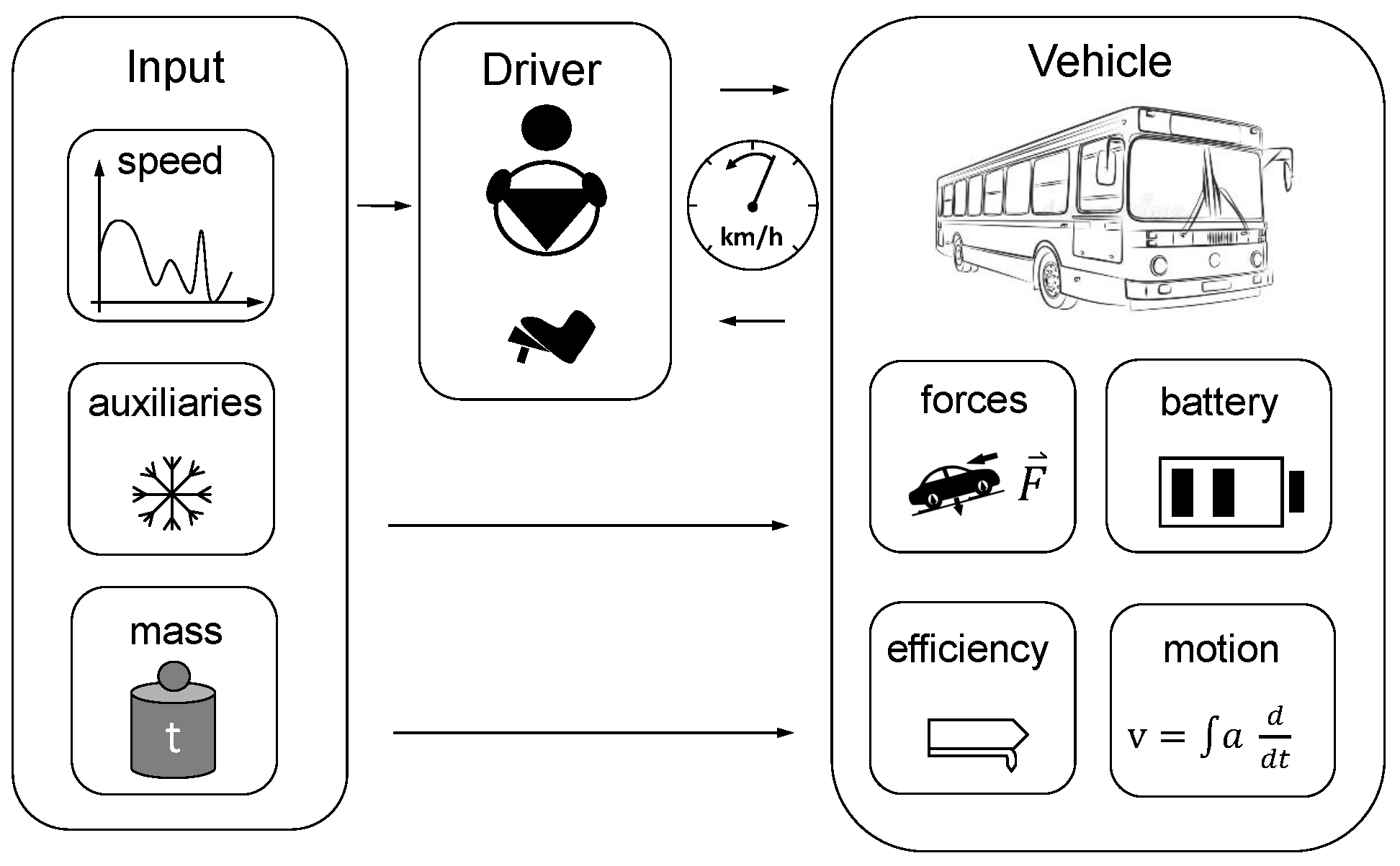
Energy Consumption Model

Figure 2 shows a simple chart of the model used in [11] to calculate the energy consumption of the BEBs, which we use as a database for this research.

The model was designed in the first place to quantify the electrical energy consumption and performance of the overall vehicle as well as different configurations of components and developed in Mathworks Simulink R2021b as a closed loop block-based model, following general modeling guidelines as described, e.g., in [35,36]. It explains the vehicle’s dynamic equations of motion (compare [37]) and the required energy flow to move the BEB from the battery to the wheels (motoring) and vice versa (recuperation). The BEB model and all its components, especially its powertrain and the mechanical body, were initially developed by the manufacturer and validated against the real testing vehicle which was supposed to operate in the target scenario. Furthermore, the model was plausibilized by an in-depth review of engineering experts in the field; in particular, the following steps of validation were performed. First, the vehicle dynamics (speed, respectively, acceleration controller, track deviation, etc.), ambient inputs and consumption rates were checked to ensure a behavior within physically plausible values. Additionally, the authors in [11] ran simulations of standardized on-road test cycles (Manhattan Bus Cycle, Braunschweig City Driving Cycle and European Transient Cycle) to assess and validate the model against comparable studies and publicly accessible real tests. Finally, all results were confirmed by the state of the art (compare, e.g., to [38,39,40,41]), and thus, the data can be considered accurate as if they had been measured experimentally by the test vehicle.

After an initial preprocessing step consisting of discarding incomplete or error-ridden records, we had 149 complete trips from twenty-four vehicles, totaling more than 2832 h of driving data (118 h per bus on average, minimum value 39.75 h, maximum value 167.25 h, standard deviation 38.1 h) available.

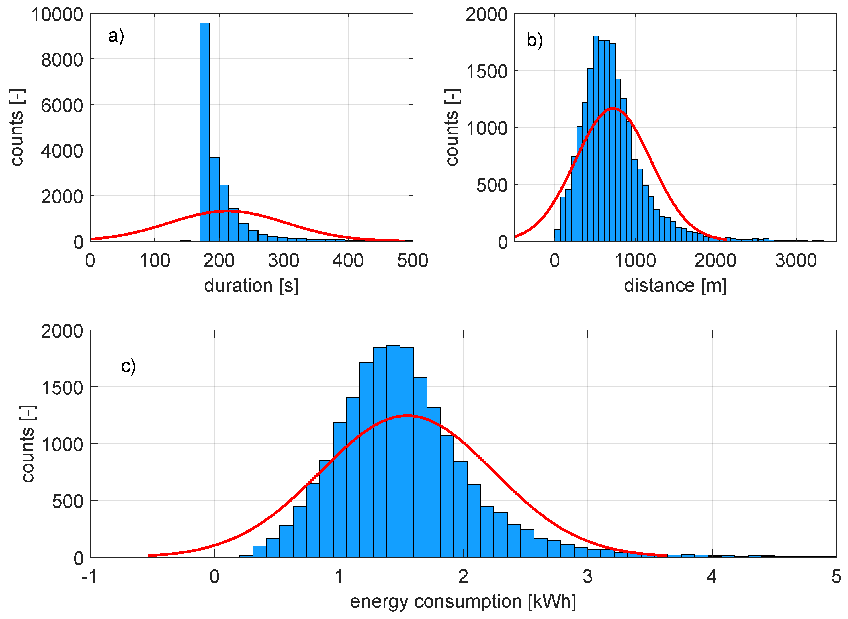
2.2. Segmentation into Microtrips

Research in the field of bus energy consumption often rests on the concept of microtrips. Such a microtrip is defined as the driving interval between two consecutive stops, and may or may not include periods of inactivity or idling. As buses often operate more than 16 h per day and cover hundreds of kilometers, this kind of segmentation is necessary to deal with the non-stationarity of driving conditions. There may be changes in the type of road (urban, suburban or highway) and in the legal speed limits, which together with traffic conditions, traffic lights, intersections, etc., influence the driving characteristics. Thus, this lack of stationarity is addressed by dividing the profile into certain partitions of approximately stationary processes, the microtrips, so that the non-stationary speed profile can be seen as a concatenation of stationary segments.

In the present paper, we define microtrips by applying three criteria for the segmentation: the speed at the beginning and end of each microtrip must be zero, $v\left(t_{start}\right)=v\left(t_{end}\right)=0$; the minimum trip length must equal 3 min, $t_{min}\ge 180$ s, and the minimum trip distance must be 50 m, $d_{min}\ge 50$ m. These values are typical for this vehicle class and in harmony with standardized driving cycles, such as the Manhattan Bus Driving Cycle (MBDC) or the Braunschweig City Driving Cycle (BCDC) (compare [42]). Figure 3 shows the distribution of duration (subplot (a)) and distance (subplot (b)) for all microtrips, which we derive using this segmentation method. It can be seen that the covered distance varies considerably from one microtrip to another, but the duration stays around 180 s in most cases.

In the end, the segmentation algorithm provided a total number of 20,297 microtrips, with an average duration of 187 s (standard deviation = 92 s) and an average distance covered of 653 m (std = 472 m). The average energy consumption is $1.5$ kWh (std = 0.7 kWh) per microtrip. Interestingly, both the Kolmogorov–Smirnov test and the Lilliefors test indicate that the data points follow Gaussian distributions in each microtrip at a significance level of $0.01$.

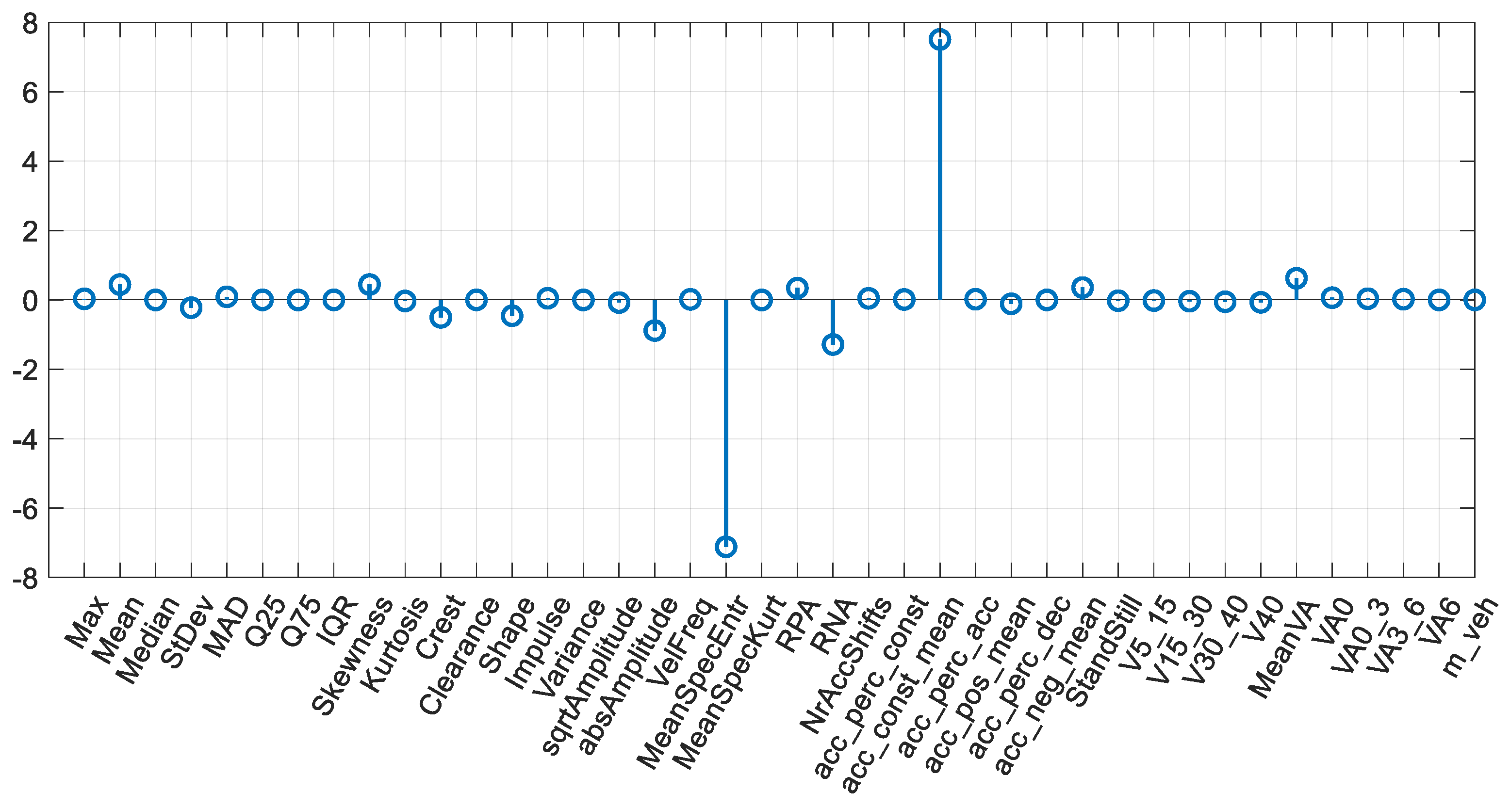
2.3. Feature Extraction

Despite the fact that energy consumption can be accurately estimated by complex physics-based models [12,13,15,16], we opt for data-based regression models based on statistics or machine learning. They can express and learn hidden, underlying relationships between speed and payload mass, on the one hand, and energy demand on the other. Once the equation is set or the model is trained, prediction from new input data is straightforward and, unlike solving physical equations numerically, facilitates real-time application, which is of high interest for the intended use case. We initially selected the 40 explanatory variables, or features, shown in

Table 1. Overview of all features used to characterize speed profiles.

Feature Name	Symbol	Unit
Maximum Speed	Max	km/h
Mean Speed	Mean	km/h
Median Speed	Median	km/h
25th Percentile	Q25	km/h
75th Percentile	Q75	km/h
Inter Quartile Range	IQR	km/h
Standstill	v0	%
Percentage of time in which $5<v\le 15$ km/h	v5_15	%
Percentage of time in which $15<v\le 30$ km/h	v15_30	%
Percentage of time in which $30<v\le 40$ km/h	v30_40	%
Percentage of time in which $v>40$ km/h	v40	%
Standard Deviation	StDev	km/h
Variance	vvariance
Mean Absolute Deviation	MAD	km/h
Skewness	vskewness	-
Kurtosis	vkurtosis	-
Crest	vcrest
Clearance	vclearance
Shape	vshape
Impulse	vimpulse
Sqrt. Amplitude	$\sqrt{v_{amp}}$
Abs. Amplitude	$|v_{amp}|$
Spectral Entropy	ventropy	-
Velocity Oscillation	vfreq	-
Number of Acceleration Shifts	nracc_shifts	-
Spectral Kurtosis	MeanSpecKurt	-
Percentage Constant Drive	accperc_const	%
Mean acceleration constant drive	accconst_mean	m/s2
Percentage Accelerating	accperc_acc	%
Mean acceleration	accpos_mean	m/s2
Percentage Decelerating	accperc_dec	%
Mean deceleration	accneg_mean	m/s2
Relative Positive Acceleration	RPA	m/s2
Relative Negative Acceleration	RNA	m/s2
1 Average $v·a$	MeanVA	m2/s3
1 Percentage of time $v·a\le 0$ m2/s3	va0	%
1 Percentage of time when $0<v·a\le 3$ m2/s3	va0_3	%
1 Percentage of time when $3<v·a\le 6$ m2/s3	va3_6	%
1 Percentage of time when $v·a>6$ m2/s3	va6	%
Total Mass (curb weight plus passengers)	mtotal	kg

¹ The product of velocity and acceleration is a surrogate for inertial and drag power [43,44].

, as the base to start from. They include common measures of tendency and variability, order statistics and non-linear descriptors. Features may also have been automatically selected from the data using techniques such as factor analysis [31], but we prefer these manually selected sets of features as they are more intuitive to interpret than machine-built ones. Consequently, all features $x_i$ with $i=[1\dots 40]$ are stored in the matrix $\mathbf{X}\in {\mathbb{R}}^{n\times i}$, where $x_{ni}$ is the $n^{th}$ observation of feature i.

$$\mathbf{X}=\left\{\begin{array}{cccc}{x}_{11}& x_{12}& \dots & x_{1i}\\ x_{21}& x_{22}& \dots & x_{2i}\\ ⋮& ⋮& \ddots & \\ x_{n1}& x_{n2}& \dots & x_{ni}\end{array}\right\}$$

(1)

On the one hand, a large number of parameters cover various characteristics, and therefore, it is more likely to identify patterns within the speed profile. On the other hand, some variables may be correlated or contain no additional information. Therefore, despite best efforts, not all features are guaranteed to have a high predictive value. Unlike complex machine learning algorithms such as neural networks, statistical approaches such as multiple linear regression cannot learn wrong interrelations and this set of features can be used causing no problems.

We finally emphasize that, whichever algorithm is used, to compare features with different units of measurement, they must first be either min-max-scaled between 0 and 1 or, as we will do in this paper, normalized to zero-mean and unit variance.

2.4. Prediction Model

In this part, we describe the regression method used to predict the energy demand $\widehat{Y}$ of the energy consumption Y. A detailed study of its development and performance is given in the Section 3.

We implement multiple linear regression (MLR), also known as multiple regression, which is essentially the extension of ordinary least-squares or linear regression. MLR is a non-learning, statistical method that allows predictions based on a set of linear functions. The model is trained, defined by as many regression parameters ${\beta }_i$ as explanatory variables $x_i$, as introduced in Section 2.3 before, plus intercept ${\beta }_0$ and offset $ϵ$. Consequently, the following linear equation system is defined:

$$\widehat{y}={\beta }_0+\sum _i{\beta }_i{x}_i+ϵ.$$

(2)

Although this approach seems simple, often good results are achieved in practice. It can be interpreted as the first baseline and assessment of the data, the predictive quality of the features and a feasibility study of the use case.

3. Experiments

The experimental results are shown in this section. All modeling, simulations and calculations were performed using MATLAB R2021b. Note that we split the complete data (20,297 microtrips) randomly into training and test sets. The major proportion of 75% is used for training and validation, while the remaining 25% is reserved for testing. During training, the models are cross-validated by 25% withheld of the training data. The quality of fit will be assessed by means of several indicators commonly used in statistics that complement each other: $r^2$, Root Mean Squared Error (RMSE) and Mean Absolute Error (MAE). They are defined as follows (3)–(6):

$$r^2=1-\frac{{\sum }_{i=1}^n{(y_i-\widehat{y})}^2}{{\sum }_{i=1}^n{(y_i-\overline{y})}^2}$$

(3)

$$MSE=\frac{1}{n}\sum _{i=1}^n{(y_i-{\widehat{y}}_i)}^2$$

(4)

$$RMSE=\sqrt{\frac{{\sum }_{i=1}^n{(y_i-{\widehat{y}}_i)}^2}{n}}$$

(5)

$$MAE=\frac{1}{n}\sum _{i=1}^n|y_i-{\widehat{y}}_i|$$

(6)

where $y_i$ is the energy consumed in the ith microtrip, ${\widehat{y}}_i$ is the ith predicted value, $\overline{y}=\frac{1}{n}{\sum }_{i=1}^n{y}_i$ and n is the total number of microtrips.

First of all, $r^2$, also called the ‘coefficient of determination’, is a metric that describes the distance between the predictions and the original data. It can be interpreted as the proportion of the variance in the response explained by the model. Its value ranges from 0 to 1 (or from 0 to 100%): the higher the value, the better the model fits the data set. MSE is the mean of the squared error and a common measure of the quality of estimation in statistics. RMSE is an intuitive and in statistics often-used metric that describes the distance from predicted values to the observed data. The lower the RMSE value, the better a model fits the dataset. Among others, RMSE has the property of having the same units as the target variable, which makes it easier to understand. Lastly, another fundamental criterion for assessing prediction models is the MAE, which is the absolute arithmetic average deviation between predicted and actual values and thus a good measure of the prediction quality.

3.1. MLR Development

First, we describe the modeling and optimization process for MLR. We use the Matlab function fitlm to implement the multiple linear regression model, which is mathematically expressed by Equation (2) with parameters that best fit according to least squares.

As a reminder of the linear model structure: $\widehat{y}={\beta }_0+x_1{\beta }_1+x_2{\beta }_2+\dots +x_i{\beta }_i+ϵ$, we analyze the model parameters $\beta$, and discover that MLR considers the spectral entropy of speed and the mean acceleration value required for constant drive most; see the following Figure 4. Interestingly, all other parameters are more or less of similar weight, which confirms the high F-statistic in the model stats, compare

Table 2. Overview of MLR model given by anova function. SumSq: Sun of squares explained by the term. DF: Degree of freedom. MeanSq: Mean square defined as $SumSq/DF$. F: F-statistic value for testing the significance of the linear terms.

	SumSq	DF	MeanSq	F	p-Value
Total	7654.5	15220	0.50292
Model	6469.9	40	174.86	2241.3	0
Residual	1184.6	15180	0.07802

. The numbers and statistics of the final model in Table 2 show also that it is significant with a p-value of 0.

3.2. Prediction Results

As the prediction of the energy consumption via MLR is based on the whole feature set (comp. Figure 1), it can be considered as a first indicator to evaluate the predictive quality of our features on the one hand and on the other a baseline against which we can compare other algorithms in future.

Table 3. Results of MLR during training (validation) and test (prediction).

MLR	Training	Test
r2	0.83	0.85
RMSE	0.35	0.27
MSE	0.12	0.07
MAE	0.18	0.18

lists the key indicators mentioned above for the model during training and validation as well as on the test data. Figure 5 shows the prediction results on the test data as well as the residuals of the MLR.

The first finding is that the coefficient of determination $r^2$ for MLR shows that this simple approach explains up to 85% of the variability of the energy consumption. Interestingly, there is no big difference in the goodness of fit for training $r_{train}^2=83\%$ and for test $r_{test}^2=85\%$, which implies the high robustness of this approach. Further, the fact that $r_{train}^2<r_{test}^2$ provokes the assumption that the split of training and test data should be shifted towards a higher training ratio. For example, 80% for training and validation and 20% for testing.

As can be seen in Figure 5, the linear approach works well for most microtrips (>97%), where consumption is between 0 and approximately 3 kWh. For microtrips with a consumption of more than 3 kWh, the deviation of predicted and real observation—the spread of error—raises and the model seems to fail to handle outliers. Particularly above 4 kWh, a constant underprediction may occur. Such systematical behavior is not captured by calculable performance indicators, which makes a deep residual analysis of any statistical or machine learning model inevitable. However, this simple straightforward approach achieves very high model fit (low bias) and excellent prediction (low variance).

4. Discussion

Recalling the importance of residual analysis, we investigate the error distribution of the model closer in Figure 6 and Figure 7 combined with

Table 4. Statistical summary of MLR residuals.

MLR	Mean Error	Std. Error	IQR	Overprediction
	0.0015	0.27	0.27	-

.

We see that the model results show no notable margin of error. Additionally, we calculated the median and skewness of the overall error distribution and found that there might be a trend of underprediction but it is almost not detectable ($<<$1%). The very low overall mean error is remarkable. Another interesting finding is that the inter-quartile range (75th–25th percentile) and the standard deviation of errors are approximately the same. This shows the homogeneity in the spread of residuals as well as the absence of outliers, respectively, and their good coverage. To buttress this result in numbers, only 17 points, which is approximately 0.3% of the complete test data, show an error $e\ge 1$.

5. Conclusions

We conclude that this statistical approach via MLR is a proper baseline to start data-based energy economy assessment for BEBs and confirms the initially formulated set of features in terms of predictive quality by means of energy consumption. Generally, the present work aims at improved mobility solutions for public transport, enhancing urban mobility’s efficiency and thus making it resource effective. Our findings can contribute to solving the socio-economic problem of electrified public transportation, which has high costs, low uncertain range and lack of infrastructure.

The main advantage of this research resides within the second stage of feature-based regression, which mainly relies on vehicle speed profiles. The necessary information is available on any vehicle platform and the low computational costs allow immediate application and are of great convenience for vehicle and fleet energy economy assessment. The overall low complexity and simplicity, particularly during training, and the high prediction accuracy and robustness underline the relevance of BEBs system design and operations planning. Furthermore, we emphasize that several stakeholders would clearly benefit from our framework. Firstly, the vehicle operator as he is provided with reliable information about the state of charge or remaining range of the BEB. Consequently, the entire fleet may be centrally monitored, managed and operated, enabling an efficient deployment. Another important group of stakeholders is the vehicle manufacturers. Exact knowledge of the energy demand is a tremendous benefit for a vehicle’s system design and would reduce safety buffers and conservative energy storage systems, which still make up to a third of vehicle costs [9]. Among others, the benefits on the highest level, e.g., for the community in Seville, can be summarized to:

• Reliable and affordable public transportation;
• Improved quality of inner-city climate;
• Overall resource effectiveness and sustainability.

On the other hand, there are also some inherent inaccuracies within this approach that are in the nature of MLR, s.a. the blurriness of prediction results or the inability to learn non-linear interrelations as, e.g., support vector machines or neural networks could do. Furthermore, the presented selection of handcrafted features is only a small fraction of a huge feature space and there may be other interesting explanatory variables of even higher predictive value that could substitute and complete the presented set. Additional metadata, such as road or weather conditions, potentially increase the prediction accuracy, which is why locally and seasonally changing conditions ought to be investigated in future research. In any case, more data will be available in the future, and thus, data-based predictive energy consumption is rising in this field. It would be interesting to investigate more and different types of features combined with other regression models and compare them against the here presented baseline.

However, all these mentioned aspects combined, and this is the important message from the presented paper, would increase the vehicle’s efficiency and thus reduce the total costs of ownership. This is finally reflected in transportation costs per mileage, which in turn has a positive impact on the final user. Affordability is key to the acceptance of alternative public transportation systems and an imminent pillar of future mobility. In summary, this huge economical, and thus in the long run environmental, leap could be realized as sustainable change emerges only from the market.

References

1. Directorate-General for Mobility and Transport (European Commission). EU Transport in Figures: Statistical Pocketbook 2019; Publications Office of the European Union: Luxembourg, 2019. [CrossRef]
2. European Parliament, Council of the European Union Directive 2009/33/EC of the European Parliament and of the Council of 23 April 2009 on the Promotion of Clean and Energy-Efficient Road Transport Vehicles. 2009. Available online: https://eur-lex.europa.eu/LexUriServ/LexUriServ.do?uri=OJ:L:2009:120:0005:0012:En:PDF (accessed on 30 April 2023).
3. Hertzke, P.; Müller, N.; Schenk, S.; Wu, T. The Global Electric-Vehicle Market is Amped up and on the Rise. EV-Volumes.com; McKinsey Analysis. 2018. Available online: https://www.mckinsey.com/industries/automotive-and-assembly/our-insights/the-global-electric-vehicle-market-is-amped-up-and-on-the-rise (accessed on 30 April 2023).
4. Braun, A.; Rid, W. Energy consumption of an electric and an internal combustion passenger car. A comparative case study from real world data on the Erfurt circuit in Germany. Transp. Res. Procedia 2017, 27, 468–475. [Google Scholar] [CrossRef]
5. Propfe, B.; Redelbach, M.; Santini, D.; Friedrich, H. Cost analysis of Plug-in Hybrid Electric Vehicles including Maintenance & Repair Costs and Resale Values. World Electr. Veh. J. 2022, 5, 886–895. [Google Scholar] [CrossRef] [Green Version]
6. Keller, V.; Lyseng, B.; Wade, C.; Scholtysik, S.; Fowler, M.; Donald, J.; Palmer-Wilson, K.; Robertson, B.; Wild, P.; Rowe, A. Electricity system and emission impact of direct and indirect electrification of heavy-duty transportation. Energy 2019, 172, 740–751. [Google Scholar] [CrossRef]
7. Koroma, M.S.; Costa, D.; Philippot, M.; Cardellini, G.; Hosen, M.S.; Coosemans, T.; Messagie, M. Life cycle assessment of battery electric vehicles: Implications of future electricity mix and different battery end-of-life management. Sci. Total Environ. 2022, 831, 154859. [Google Scholar] [CrossRef] [PubMed]
8. Kalghatgi, G. Is it really the end of internal combustion engines and petroleum in transport? Appl. Energy 2018, 225, 965–974. [Google Scholar] [CrossRef]
9. König, A.; Nicoletti, L.; Schröder, D.; Wolff, S.; Waclaw, A.; Lienkamp, M. An Overview of Parameter and Cost for Battery Electric Vehicles. World Electr. Veh. J. 2021, 12, 21. [Google Scholar] [CrossRef]
10. Lajunen, A.; Lipman, T. Lifecycle cost assessment and carbon dioxide emissions of diesel, natural gas, hybrid electric, fuel cell hybrid and electric transit buses. Energy 2016, 106, 329–342. [Google Scholar] [CrossRef]
11. Sennefelder, R.M.; Micek, P.; Martin-Clemente, R.; Risquez, J.C.; Carvajal, R.; Carrillo-Castrillo, J.A. Driving Cycle Synthesis, Aiming for Realness, by Extending Real-World Driving Databases. IEEE Access 2022, 10, 54123–54135. [Google Scholar] [CrossRef]
12. Asamer, J.; Graser, A.; Heilmann, B.; Ruthmair, M. Sensitivity analysis for energy demand estimation of electric vehicles. Transp. Res. Part Transp. Environ. 2016, 46, 182–199. [Google Scholar] [CrossRef]
13. De Cauwer, C.; Van Mierlo, J.; Coosemans, T. Energy Consumption Prediction for Electric Vehicles Based on Real-World Data. Energies 2015, 8, 8573–8593. [Google Scholar] [CrossRef] [Green Version]
14. Gallet, M.; Massier, T.; Hamacher, T. Estimation of the energy demand of electric buses based on real-world data for large-scale public transport networks. Appl. Energy 2018, 230, 344–356. [Google Scholar] [CrossRef]
15. Wang, J.; Besselink, I.; Nijmeijer, H. Battery electric vehicle energy consumption modelling for range estimation. Int. J. Electr. Hybrid Veh. 2017, 9, 79–102. [Google Scholar] [CrossRef]
16. Beckers, C.; Besselink, I.; Frints, J.; Nijmeijer, H. Energy consumption prediction for electric city buses. In Proceedings of the 13th ITS European Congress, Brainport, The Netherlands, 3–6 June 2019; pp. 3–6. [Google Scholar]
17. Hjelkrem, O.A.; Lervåg, K.Y.; Babri, S.; Lu, C.; Södersten, C.J. A battery electric bus energy consumption model for strategic purposes: Validation of a proposed model structure with data from bus fleets in China and Norway. Transp. Res. Part D Transp. Environ. 2021, 94, 102804. [Google Scholar] [CrossRef]
18. Maybury, L.; Corcoran, P.; Cipcigan, L. Mathematical modelling of electric vehicle adoption: A systematic literature review. Transp. Res. Part D Transp. Environ. 2022, 107, 103278. [Google Scholar] [CrossRef]
19. Chen, Y.; Wu, G.; Sun, R.; Dubey, A.; Laszka, A.; Pugliese, P. A Review and Outlook on Energy Consumption Estimation Models for Electric Vehicles. Sae Int. J. Sustain. Transp. Energy Environ. Policy 2021, 2, 79–96. [Google Scholar] [CrossRef]
20. Lajunen, A. Energy consumption and cost-benefit analysis of hybrid and electric city buses. Transp. Res. Part Emerg. Technol. 2014, 38, 1–15. [Google Scholar] [CrossRef]
21. Vepsäläinen, J.; Otto, K.; Lajunen, A.; Tammi, K. Computationally efficient model for energy demand prediction of electric city bus in varying operating conditions. Energy 2019, 169, 433–443. [Google Scholar] [CrossRef]
22. Abdelaty, H.; Mohamed, M. A Prediction Model for Battery Electric Bus Energy Consumption in Transit. Energies 2021, 14, 2824. [Google Scholar] [CrossRef]
23. Abdelaty, H.; Al-Obaidi, A.; Mohamed, M.; Farag, H.E. Machine learning prediction models for battery-electric bus energy consumption in transit. Transp. Res. Part D Transp. Environ. 2021, 96, 102868. [Google Scholar] [CrossRef]
24. Pamuła, T.; Pamuła, D. Prediction of Electric Buses Energy Consumption from Trip Parameters Using Deep Learning. Energies 2022, 15, 1747. [Google Scholar] [CrossRef]
25. Abdelaty, H.; Mohamed, M. A framework for BEB energy prediction using low-resolution open-source data-driven model. Transp. Res. Part D Transp. Environ. 2022, 103, 103170. [Google Scholar] [CrossRef]
26. Basso, R.; Kulcsár, B.; Sanchez-Diaz, I. Electric vehicle routing problem with machine learning for energy prediction. Transp. Res. Part Methodol. 2021, 145, 24–55. [Google Scholar] [CrossRef]
27. Sun, C.; Sun, F.; He, H. Investigating adaptive-ECMS with velocity forecast ability for hybrid electric vehicles. Appl. Energy 2017, 185, 1644–1653. [Google Scholar] [CrossRef]
28. Liu, Y.; Li, J.; Gao, J.; Lei, Z.; Zhang, Y.; Chen, Z. Prediction of vehicle driving conditions with incorporation of stochastic forecasting and machine learning and a case study in energy management of plug-in hybrid electric vehicles. Mech. Syst. Signal Process. 2021, 158, 107765. [Google Scholar] [CrossRef]
29. Aljohani, T.M.; Ebrahim, A.; Mohammed, O. Real-Time metadata-driven routing optimization for electric vehicle energy consumption minimization using deep reinforcement learning and Markov chain model. Electr. Power Syst. Res. 2021, 192, 106962. [Google Scholar] [CrossRef]
30. Kontou, A.; Miles, J. Electric Buses: Lessons to be Learnt from the Milton Keynes Demonstration Project. Procedia Eng. 2015, 118, 1137–1144. [Google Scholar] [CrossRef] [Green Version]
31. Ericsson, E. Independent driving pattern factors and their influence on fuel-use and exhaust emission factors. Transp. Res. Part D Transp. Environ. 2001, 6, 325–345. [Google Scholar] [CrossRef]
32. Simonis, C.; Sennefelder, R. Route specific Driver Characterization for Data-Based Range Prediction of Battery Electric Vehicles. In Proceedings of the 2019 Fourteenth International Conference on Ecological Vehicles and Renewable Energies (EVER), Monte-Carlo, Monaco, 8–10 May 2019; pp. 1–6. [Google Scholar] [CrossRef]
33. Li, P.; Zhang, Y.; Zhang, Y.; Zhang, Y.; Zhang, K. Prediction of electric bus energy consumption with stochastic speed profile generation modelling and data driven method based on real-world big data. Appl. Energy 2021, 298, 117204. [Google Scholar] [CrossRef]
34. Chen, Y.; Zhang, Y.; Sun, R. Data-driven estimation of energy consumption for electric bus under real-world driving conditions. Transp. Res. Part D Transp. Environ. 2021, 98, 102969. [Google Scholar] [CrossRef]
35. Hahn, B.H.; Valentine, D.T. Essential MATLAB for Engineers and Scientists; Elsevier: Amsterdam, The Netherlands, 2017. [Google Scholar] [CrossRef] [Green Version]
36. Markel, T.; Brooker, A.; Hendricks, T.; Johnson, V.; Kelly, K.; Kramer, B.; O’Keefe, M.; Sprik, S.; Wipke, K. ADVISOR: A systems analysis tool for advanced vehicle modeling. J. Power Sources 2022, 110, 255–266. [Google Scholar] [CrossRef]
37. Rajamani, R. Longitudinal Vehicle Dynamics. In Vehicle Dynamics and Control; Springer: New York, NY, USA, 2006; pp. 95–122. [Google Scholar] [CrossRef]
38. Kivekäs, K.; Lajunen, A.; Vepsäläinen, J.; Tammi, K. City Bus Powertrain Comparison: Driving Cycle Variation and Passenger Load Sensitivity Analysis. Energies 2018, 11, 1755. [Google Scholar] [CrossRef] [Green Version]
39. Göhlich, D.; Fay, T.A.; Jefferies, D.; Lauth, E.; Kunith, A.; Zhang, X. Design of urban electric bus systems. Des. Sci. 2018, 4. [Google Scholar] [CrossRef] [Green Version]
40. Gao, Z.; Lin, Z.; LaClair, T.J.; Liu, C.; Li, J.M.; Birky, A.K.; Ward, J. Battery capacity and recharging needs for electric buses in city transit service. Energy 2017, 122, 588–600. [Google Scholar] [CrossRef] [Green Version]
41. Göhlich, D.; Kunith, A.; Ly, T.A. Technology Assessment of an Electric Urban Bus System for Berlin; WIT Press: Southampton, UK, 2014; Volume 138. [Google Scholar] [CrossRef] [Green Version]
42. Barlow, T.; Latham, S.; McCrae, I.S.; Boulter, P. A reference book of driving cycles for use in the measurement of road vehicle emissions. In TRL Published Project Report; TRL Limited: Wokingham, UK, 2009. Available online: https://assets.publishing.service.gov.uk/government/uploads/system/uploads/attachment_data/file/4247/ppr-354.pdf (accessed on 30 April 2023).
43. Fomunung, I.; Washington, S.; Guensler, R. A statistical model for estimating oxides of nitrogen emissions from light duty motor vehicles. Transp. Res. Part D Transp. Environ. 1999, 4, 333–352. [Google Scholar] [CrossRef]
44. Huang, D.; Xie, H.; Ma, H.; Sun, Q. Driving cycle prediction model based on bus route features. Transp. Res. Part D Transp. Environ. 2017, 54, 99–113. [Google Scholar] [CrossRef]
Figure 1. Graphical abstract of the papers methodology.
Energies 16 04365 g001
Figure 2. Schematic of the vehicle longitudinal dynamics simulation model used in [11] to calculate the electrical energy consumption. Set of three inputs: speed, auxiliary power and mass. The driver acts as a speed/acceleration controller. The vehicle model translates the torque into electrical power demand from the battery and integrates the driving forces to move the vehicle. Its speed is fed back to the driver where the loop closes.
Energies 16 04365 g002
Figure 3. Distribution of traveled time (subplot (a)) and distance (subplot (b)) per microtrip for the entire database (20,297 microtrips) as well as the corresponding consumed energy (subplot (c)).
Energies 16 04365 g003
Figure 4. Parameter weights of MLR. Spectral entropy and mean acceleration value for constant drive are considered most.
Energies 16 04365 g004
Figure 5. Prediction results of MLR on test data. Color bar shows the residuals, which is the error e between real observation y and predicted value y ^ .
Energies 16 04365 g005
Figure 6. Boxplot and scattered errors of MLR prediction results.
Energies 16 04365 g006
Figure 7. Overview of residuals and distribution of error.
Energies 16 04365 g007