Abstract
Pulse tube refrigerators are widely used in certain special fields, such as aerospace, due to their unique advantages. Compared to a conventional phase shifter, the active displacer helps to achieve a higher cooling efficiency for pulse tube refrigerators. At present, the displacer is mainly studied by one-dimensional simulation, and the optimization method is not perfect due to its poor accuracy, which is not conducive to obtaining a better performance. Based on the current status of displacer research, phase-shift mechanisms of inertance tube pulse tube refrigerators and active displacer pulse tube refrigerators were firstly studied comparatively by multidimensional simulation, and then we determined the crucial effect properties that lead to a better cooling performance for the active displacer pulse tube refrigerator at different cooling temperatures. Finally, an efficient optimization method combining the Kriging model and genetic algorithm is proposed to further improve the cooling performance of the active displacer pulse tube refrigerator. The results show that the active displacer substantially improves the cooling performance compared to the inertance tube mainly by increasing the PV power and enthalpy flow in the pulse tube. The Kriging agent models of active displacer pulse tube refrigerator achieve 98.2%, 98.31%, 97.86%, and 97.32% prediction accuracy for no-load temperature, cooling capacity, coefficient of performance, and total input PV power, respectively. After optimization, the no-load temperature is minimally optimized for a 23.68% reduction compared to the initial one with a relatively high efficiency, and the founded optimization methods can also be weighted for multiple objectives, according to actual needs.
1. Introduction
Pulse tube refrigerators (PTRs) feature no moving parts and possess low mechanical vibration at low temperatures, leading to their widespread use for the cooling of high-precision detectors due to their long lifetime and high reliability [1,2,3]. Since the original basic PTR [4] was proposed, with the update of the phase-shift mechanism, the performance of the PTR has been effectively improved, such as orifice PTR [5,6], double inlet PTR [7], and inertance tube PTR [8]. Recently, the PTR with a new phase-shift structure named active displacer emerged and was widely concerned for its effective function in phase shift [9,10].
For active displacer pulse tube refrigerators (ADPTRs), Shi [11] firstly made the study of PTR with a rod-type displacer experimentally and achieved a no-load temperature of 38.9 K, which verified the feasibility of this phase-shift structure and has now gained a wide range of applications in coaxial PTRs [12,13], two-stage PTRs [14,15,16], hybrid Stirling/pulse tube refrigerators [17,18], etc. The displacer as phase shifter can achieve the function of effectively improving the cooling performance of the refrigerator compared with the traditional phase-shift method. The experimental results of Zhu [15] showed that the relative Carnot efficiency at a 30 K cooling temperature increased from 5.3% to 6.64% when the piston phase shifter was applied to the refrigerator system after replacing the inertance tube and reservoir. Pang [16] experimentally compared the displacer with the double inlet structure, and the relative Carnot efficiency (RCOP) of the refrigerator increased from 3.85% to 6.5% at the temperature of 20 K when the former shifter was applied. In order to comprehend the working mechanism of the displacer in improving the efficiency of the PTR, scholars have performed more detailed studies on the inside of the cold finger. Abolghasemi [19] investigated the phase angle between pressure wave amplitude and mass flow rate amplitude within the refrigerator through one-dimensional simulations, which showed that the main reason for the displacer to improve cooling performance is not achieved by shifting the phase angle between the pressure and the flow but by increasing the mass flow rate amplitude at the end of the pulse tube. In order to investigate the impact of the displacer on improving the cooling performance of the PTR, Chen [20] applied an acoustic impedance model and kinetic model and verified via an experiment. Deng [21] proposed an electroacoustic circuit model for optimizing the operating state based on the thermoacoustic theory. The current theoretical research on the ADPTR is mainly focused on one-dimensional simulation, which has the advantage of high computational efficiency, as well as notable disadvantages of not intuitively and inaccurately reflecting the actual flow and heat-transfer characteristics, which can be better presented by multidimensional modeling. Based on the limitations of the current research approach on ADPTR, we will further investigate the differences in flow and heat transfer characteristics of the working fluid between the ADPTR and the inertance tube pulse tube refrigerator (ITPTR) by using a multidimensional flow simulation method with higher computational accuracy to reveal the internal mechanism of the superiority of its cooling effect over ITPTR.
The mechanism study of the ADPTR can provide a direction for the improvement of its cooling performance, based on which, scholars have performed a lot of optimization work for their structural parameters, such as the displacement of the displacer and phase angle between piston of the compressor and displacement of the displacer [12], the frequency and key parameters of displacer [20], and the length of pulse tube and regenerator [13] in recent years. However, the current optimization method applied to the ADPTR is based on the linear variation of the optimization target with each operating parameter, which may not be so ideal in practice and presents a more complex variation pattern making the optimization more difficult. Therefore, a more scientifically rigorous optimization algorithm of the combination of artificial intelligence optimization algorithms and efficient agent modeling has be applied to PTRs, such as the combination of Response Surface Methodology (RSM) and Non-Sorted Genetic Algorithm II to optimize ITPTR [22], artificial neural network and particle swarm optimization to optimize orifice PTR [23], and artificial neural network (ANN) model to predict and optimize compressor operating condition of ITPTR [24]. The abovementioned main application object of the optimization design research is still focused on PTR with a traditional phase shifter, where there are few studies related to the optimization of design parameters for the ADPTR, and we will perform a further in-depth analysis of the ADPTR with more advanced optimization algorithms in the future.
Although the above RSM and ANN models for PTR structural parameters can improve the optimization efficiency of PTR parameters, there are still shortcomings in the accuracy and efficiency of the modeling process, especially for ADPTRs with complex phase-shift structures, while the Kriging meta-modeling makes up for the deficiencies and is well suited for the design and optimization of ADPTR. Krige first proposed Kriging meta-modeling [25] and is now widely used in various engineering fields of research due to its generality and accuracy. Yang [26] compared five metamodels for the vehicle crash design problem and found that the Kriging meta-model has better accuracy for predicting the key performance index of toe-board intrusion in vehicle crash with a root mean square error of 0.9%. Prebeg [27] conducted extensive tests on a simple barge and demonstrated that the Kriging meta-model can be used with sufficient accuracy for structural design. Zheng [28] used a Kriging meta-model and genetic algorithm to make a correction for the space instrument thermal model, and the average temperature error of the two components after the correction was reduced from 5.57% to 3.23% and 25.53% to 11.57%, respectively. In summary, due to the high accuracy and efficiency of the optimization method combining Kriging model and genetic algorithm, it is more applicable to the optimization of the ADPTR, and this method was used for the optimization study of ADPTR in this paper.
Based on the current state of research, we developed a two-dimensional model for the conventional ITPTR and the ADPTR with excellent cooling performance, computational fluid dynamics (CFD) multidimensional simulations were performed to analyze and compare their flow and heat-transfer characteristics within the cold finger. Two key parameters of the displacer of the ADPTR, namely the maximum piston displacement (xd) and the phase angle (θ) of the displacer, were further analyzed, and the optimization of these two variables was accomplished through the Kriging agent model combined with the Non-Sorted Genetic Algorithm, with the aim of obtaining a lower no-load temperature and higher cooling capacity of the ADPTR. A CFD analysis of the ADPTR helps to gain insight into its cooling mechanism, and the optimization results may provide new and simpler design optimization ideas for ADPTR.
2. Theoretical Analysis
2.1. Numerical Modeling
The two-dimensional axisymmetric models established for ITPTR and ADPTR are shown in Figure 1; the displacer is equivalent to a phase-shift single side compressor, and its motion parameters can be controlled by electrical parameters. The geometric parameters and boundary conditions of all components in the two models are shown in Table 1.
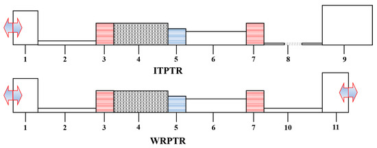
Figure 1.
Physical model of ITPTR and ADPTR: (1) compressor; (2) transfer line 1; (3) after cooler (WHX1); (4) regenerator; (5) cold end heat exchanger (CHX); (6) pulse tube; (7) hot end heat exchanger (WHX2); (8) inertance tube; (9) reservoir; (10) transfer line 2; and (11) displacer.

Table 1.
Geometry details and boundary conditions.
The commercial CFD software ANASYS Fluent was used to simulate the above PTR model. Since both the compressor and displacer need to be simulated for the motion of the piston, and there exists a phase angle between two pistons of the compressor and displacer, making the motion of the two pistons not synchronizing, a dynamic mesh is used to simulate the motion of the piston.
Displacement of compressor piston:
where ω = 2πf; f is the operating frequency of pistons in the compressor and displacer with a magnitude of 34 Hz; Xc is the piston displacement of the compressor; xc is the maximum value of the piston displacement of the compressor with a magnitude of 4.511 mm; and the displacement of the displacer piston is
where Xd is the piston displacement of the displacer, xd is the maximum value of the piston displacement of the displacer with a magnitude of 1.5 mm, and θ is the phase angle between them in operation with a magnitude of 220°.
The governing equations solved by Fluent for helium in the refrigerator simulation are as follows:
where ε is the porosity, taking the value as 1 for the hollow tube region, such as the pulse tube, connecting tube, and inertance tube, and is simulated using the SST turbulence model with high computational accuracy, i.e., 0.69, for the porous media region, such as the heat exchanger and regenerator, and is simulated using the laminar flow model due to its small Reynolds number, with copper as the solid phase material of the heat exchanger, and SS-304 as the solid phase material of the regenerator. Moreover, ρf, , p, σ, Ef, and kf are the density, velocity vector, pressure, stress tensor, energy, and the thermal conductivity of helium, respectively. Si is the resistance source term in the momentum equation, which only needs to be considered in the porous media region and can be expressed as follows:
where μ is the viscosity, α is the permeability with a value of 1.06 × 10⁻¹⁰ m2, and C2 is the initial resistance factor with a value of 76,090 m−1 [29]. The initial charge pressure and initial temperature of the whole refrigerator are 3.1 MPa and 300 K, respectively. The pressure solver was used to solve the problem; the coupling scheme of pressure and velocity is PISO; the spatial dispersion scheme of pressure is PRESTO; and the second-order upwind scheme was used for the density, momentum, and energy. For the energy equation, the convergence tolerance criterion is 1 × 10⁻⁶, and the rest of the items are 1 × 10⁻³. ANASYS Icem was used to delineate the quadrilateral grid for the PTR model, the minimum mesh size at the boundary layer is 0.1 mm, and the grid far away from the boundary layer is no more than 0.8 mm, while the reservoir does not need high calculation accuracy that the grid is larger. The aspect ratio of the each element is no more than 1:3, and the numbers of grids used for the calculation of the ITPTR and ADPTR are 7189 and 4730, respectively. As demonstrated in Figure 2, the heat flux rate on the CHX wall of PTRs varies with the number of mesh at a cooling temperature of 110 K. Due to the difference in the calculation accuracy, the heat flux rate at the CHX wall will increase as the mesh quantity decreases, and there is no significant difference as the number of grids is increased to 9000 and 5800 accordingly, which indicates that the number of grids fully satisfies the calculation accuracy.
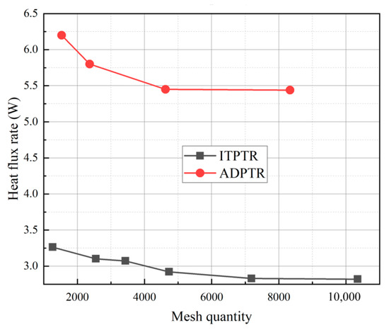
Figure 2.
Verification of mesh quantity independence for numerical models.
As an electrically driven compressor, the internal PV power of displacer is also a part of the total input PV power, and the total input PV power (W) can be expressed as follows:
where Wd is the PV power at the displacer, and Wc is the PV power at the compressor. The calculation expression for PV power is as follows:
where ΔP is the amplitude of pressure, ΔV is the amplitude of volume flow rate, and β is phase angle between them.
Based on the first law of thermodynamics and the second law of thermodynamics, Radebaugh derived the enthalpy and entropy flow model [30] for the PTR, which exactly explained the cooling mechanism of the PTR and was widely accepted and used to calculate the cooling power and analyze various losses of PTRs. At the cold end, there is no input and output work. Then, the cooling capacity can be expressed as follows:
where Qc is the cooling capacity, and and are the time-averaged enthalpy flow in the pulse tube and regenerator, respectively. The time-averaged enthalpy flow can be calculated as follows:
where τ is the duration of the cycle, is the mass flow, Cp is the heat capacity, h is the specific enthalpy, and T is the temperature.
is zero for an ideal gas and an ideal regenerator, while for an actual regenerator, is considered to be a loss. For an actual pulse tube, turbulence causes irreversible reactions inside and results in non-ideal expansion loss. According to the second law of thermodynamics, the can be expressed as follows:
where Wpt is the PV power, and is the non-ideal expansion loss.
The figure of merit (FOM) can be used to quantify the loss in the pulse tube:
The coefficient of performance (COP) and RCOP can be used to evaluate the cooling efficiency of ITPTR and ADPTR. The formulas are as follows:
where Tw and Tc are the temperature at hot end and cold end of the pulse tube, respectively; for ITPTR, W is the PV power at the compressor, and for ADPTR, W is the sum of the PV power at the compressor and displacer.
2.2. Kriging-Meta-Modeling Method Combined with Genetic Algorithm
Using the CFD simulation alone to optimize the PTR will consume a lot of computational resources. As the agent model of the original numerical model, the Kriging meta model is a more efficient solver of the target output, so it is usually used to perform the iterative calculation of the genetic algorithm. In the optimal design, the sample set was first extracted by the Latin Hypercube Sampling (LHS) method, and the mathematical relationship between the independent variables and the response quantities was established as a Kriging model [28]. Their functional relationship is shown below.
where fj(x) is the polynomial basis function, which can be constructed by using the global approximation model constructed from the sample points. βj(x) and ε(x) are the regression parameter and the error function of the random distribution with the following distribution law.
where E[ε(x)] is the expectation, Var[ε(x)] is the variance, and Cov[ε(xi), ε(xj)] is the covariance. Moreover, xi and xj are any two training sample points, and R(θ, xi, xj) is the function used to represent the spatial correlation between the sample points, and the specific expression is shown below.
where θ is the model-related parameter, xip and xjp are the sample points in p dimensions, and the regression parameters and variance are estimated as in Equations (20) and (21).
where F is a matrix consisting of vectors of basis function f(x), i.e., F = [f1(x), f2(x), …, fn(x)], and R is defined as follows.
Using the obtained model-related parameters, the prediction can be made for any point in the sample interval, as shown below.
According to the existing sample points and the predicted sample points, the vector relationship constructed is shown below:
The accuracy of the Kriging model is evaluated by constructing the relationship between the true value, f, and the predicted value, , i.e., the Root Mean Square Error (RMSE), through Equation (25).
After the Kriging model constructs a response surface with sufficient accuracy based on the simulated data, the optimal target value can be found by the genetic algorithm. The basic idea of the genetic algorithm is to continuously extract samples from the Kriging model, and after a certain number of iterations, to obtain the optimal solution of the sample close to the actual problem, take the example of minimizing the no-load temperature at the cold end of the PTR. The objective function set by the genetic algorithm optimization is shown in Equation (26), and the optimization flowchart of the combination of the Kriging model and genetic algorithm is shown in Figure 3.
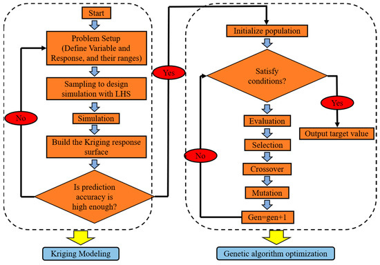
Figure 3.
Flowchart of the analysis and optimization process.
3. Comparisons between the ADPTR and ITPTR
3.1. Comparison of the Cooling Performance of ITPTR and ADPTR
The variation curve of the wall temperature of the CHX with time is illuminated in Figure 4. The no-load temperature of the ITPTR reaches equilibrium at 74 K, which agrees well with the simulation results of Chen et al. [31], while ADPTR is significantly superior to ITPTR, with an equilibrium temperature of 52.4 K.
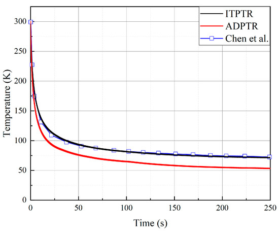
Figure 4.
Variation of wall temperature with time for CHX in the simulation.
To further comprehend the difference in the cooling performance between the ITPTR and ADPTR, the walls of the cold-end heat exchanger are set to the boundary condition of the constant temperature to compare their cooling performance in the five cooling temperatures of 90 K, 110 K, 130 K, 150 K, and 170 K. The main difference between the ADPTR and ITPTR is that the displacer can effectively adjust the phase relationship between the pressure and flow inside the cold finger to improve the cooling efficiency of ADPTR, while the phase shifter of the ITPTR is the inertance tube and reservoir, making its phase-shift ability is not as good as that of the displacer.
Since the displacer is an electrically driven compressor, the total input PV power of PTRs will increase when it is used as a phase shifter, as shown in Figure 5a, the red line indicates the cooling capacity, which can be seen that the cooling capacity increases as a result. The total input PV power of ADPTR at each cooling temperature is 10~20 W higher than that of the ITPTR, and the cooling capacity is also increased by approximately 2.5~3.3 W higher than that of the ITPTR due to the increased PV power in the pulse tube with the displacer, and the cooling capacity of both PTRs increases with the increase of the cooling temperature.
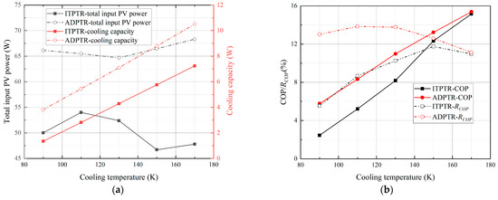
Figure 5.
Variation of working performance parameters with cooling temperature: (a) PV power and cooling capacity; and (b) COP and RCOP.
The variations of COP and RCOP with cooling temperature for both ITPTR and ADPTR are expressed in Figure 5b, again demonstrating that the excellent phase-shift ability of the displacer improves the cooling performance. As the displacer shifts the phase relationship within the PTR to a better state, the total loss of the cold finger is reduced; thus, the COP and RCOP of the ADPTR are always higher than that of the ITPTR, as the cooling temperature varies. Moreover, the difference between the two increases at lower temperatures, and the COP and the RCOP of the ADPTR are higher than ITPTR by 3.32% and 7.49% when cooling at 90 K, respectively, while the difference between the two in cooling efficiency gradually shrinks to zero at 170 K.
3.2. Analysis of Losses within the Cold Finger
The excellent phase-shift ability of the displacer has been widely studied by scholars, but the impact of displacer on the internal loss of the cold finger has been less studied. The losses within the PTR mainly occur in the regenerator and the pulse tube. The high-pressure oscillating flow gas will cause pressure-drop losses and enthalpy-flow losses due to the axial heat conduction of gas and solid in the regenerator, while irreversible processes will also occur in the pulse tube, causing non-ideal expansion losses, mainly including heat-transfer losses between the gas and wall of the pulse tube, the mixing of hot and cold gases caused by turbulence.
Figure 6a,b show the pressure and mass flow rate amplitude distribution of the ADPTR and ITPTR at different cooling temperatures inside the regenerator. Since the losses of the regenerator decrease as the cooling temperature increases and the losses for ADPTR are lower than ITPTR, the pressure amplitude increases with the increase of the cooling temperature, and the pressure amplitude of the ADPTR is always much higher than that of the ITPTR, which could transmit higher PV power. The mass flow amplitude decreases with the increasing of the cooling temperature, and the mass flow amplitude of ADPTR is always lower than that of ITPTR. Since most of the losses in the regenerator are positively related to the mass flow rate, a lower mass flow amplitude is beneficial to reduce the losses in the regenerator. The enthalpy flow loss in the regenerator for the ADPTR and ITPTR as the cooling temperature varies is shown in Figure 6c. Due to the better phase relationship of the regenerator at lower cooling temperatures caused by the displacer, as the cooling temperature increases, the enthalpy flow loss in the regenerator of the ADPTR and ITPTR shows a completely different trend, with the enthalpy flow loss of ADPTR increasing from 1.08 W at 90 K to 1.34 W at 170 K, while the enthalpy flow loss of ITPTR decreases from 1.64 W at 90 K to 1.22 W at 170 K. Figure 6d denotes the PV power and enthalpy flow of ITPTR and ADPTR inside the pulse tube at different cooling temperatures. Both of them increase with the cooling temperature increasing, and the ADPTR always has higher PV power and enthalpy flow. While the red line indicates the FOM, FOM can be calculated according to Equation (12); the pulse tube FOM of the ADPTR rises from 50.3% at 90 K to 70.2% at 170 K; and for the ITPTR, it rises from 51.5% at 90 K to 80.3% at 170 K, which is always higher than that of the ADPTR due to its lower the non-ideal expansion loss than that of the ADPTR. In summary, the displacer can increase the PV power by 67.2%, 77.7%, 66.1%, 55.5%, and 60.1% at 90 K, 110 K, 130 K, 150 K, and 170 K temperatures, respectively, while on the other hand, it leads to a negative effect on FOM due to the enhanced turbulence in pulse tube. The key point for the ADPTR to significantly improve the cooling performance is that the increase in non-ideal expansion loss can be covered by the increase in the enthalpy flow of the pulse tube.
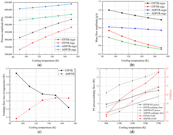
Figure 6.
Variation of working parameters inside the cold finger with cooling temperature: (a) pressure amplitude in the regenerator, (b) mass flow amplitude in the regenerator, (c) enthalpy flow loss in the regenerator, and (d) PV power and enthalpy flow in the pulse tube.
3.3. Flow and Heat Transfer Characteristics in the Pulse Tube
To analyze in detail the causes of the low FOM of ADPTR, a two-dimensional analysis of flow and heat transfer of the pulse tube is required. Taking the 90 K cooling temperature as an example, the axial temperature variation within one cooling cycle in the pulse tubes of the ADPTR and ITPTR is shown in Figure 7. The maximum temperature at the hot end of ADPTR can reach 324 K, higher than the 309 K of ITPTR, and the temperature fluctuation is more dramatic throughout the axial direction, especially at the hot end, where the temperature fluctuation range reaches the maximum. This is due to the pushing action of the piston inside the displacer, which triggers higher velocities in the pulse tube, especially at the hot end, where the increase in velocity is more pronounced. Figure 8 shows the temperature contours for both pulse tubes, giving a gorgeous indication of the fluctuations in space after temperature stabilization, which is also a multidimensional perspective on the presentation of the phenomenon depicted in Figure 7.
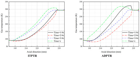
Figure 7.
Axial temperature variation within one cycle of the pulse tube.
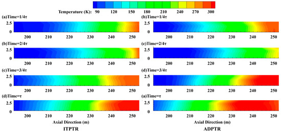
Figure 8.
Temperature contour of the pulse tube.
The more intense turbulence in the pulse tube of the ADPTR leads to differences in its temperature distribution with that of the ITPTR. The axial velocity distribution along the radial direction inside the pulse tube is shown in Figure 9. It can be seen that the velocities of ADPTR and ITPTR show a slight difference at the inlet of the pulse tube, and then the velocity of ADPTR becomes larger in the middle and reaches the maximum at the outlet, while that of ITPTR experiences an opposite process, which becomes smaller and reaches the minimum at the outlet. The velocity gradient of the ADPTR is also larger near the wall, which is mainly caused by the more intense jet. The stronger jet in the pulse tube of the ADPTR is mainly caused by the reciprocating motion of the displacer piston, which may be the main disadvantage of the ADPTR compared to the ITPTR during refrigeration. The vortex images in Figure 10 interpretate the cases of the vorticity in the pulse tube of the ADPTR and ITPTR, where the vorticity arises at the inlet of the pulse tube, triggered by the Rayleigh flow near the wall, and extends backwards with the flow, reaching its maximum at the outlet of the pulse tube. The vorticity magnitude contour is a good parameter to describe the flow nonlinear process, and due to the displacer, the ADPTR presents a stronger jet influence at the outlet of the pulse tube. The optimization of the flow in the cold finger of the ADPTR becomes particularly important by observing the presentation of turbulent flow in the pulse tube of Figure 7, Figure 8, Figure 9 and Figure 10.
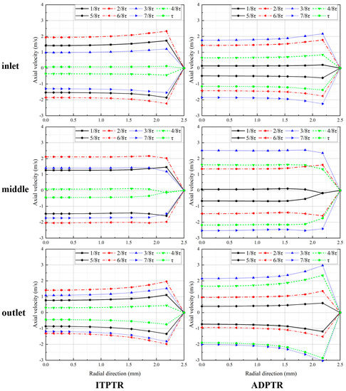
Figure 9.
Velocity distribution at the inlet, middle, and outlet of the pulse tube.
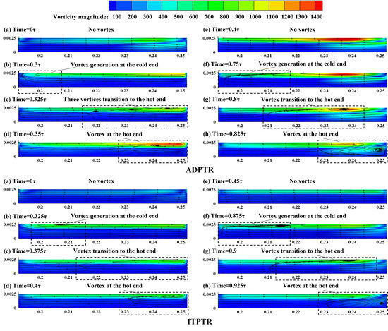
Figure 10.
Vortex in the pulse tube.
4. Optimization of Displacer Parameters for ADPTR
From the previous comparative analysis of ITPTR and ADPTR, the displacer displayed an excellent phase-shift ability, thereby reducing various losses within the cold finger, which leads to a significant improvement in cooling performance achieved by the ADPTR, and numerous studies [12,19,20] have been conducted to prove that the key factors affecting the phase relationship in the cold finger are the maximum displacement (xd) of the displacer and the phase angle (θ) between the pistons of displacer and the compressor, which needs to be further optimized.
4.1. Effect of the xd and θ
Figure 11a demonstrates the variation of the wall temperature of CHX with time, where xd is taken as 1.1 mm, 1.3 mm, 1.5 mm, 1.7 mm, and 1.9 mm; and θ is taken as a constant value of 220°. In order to accelerate the iteration speed, a linear temperature distribution from 80 K to 300 K is set in both regenerator and pulse tube. The final stable temperature at xd = 1.5 mm is 51.1 K, while the final stable temperature for cooling from the 300 K temperature field is 52.44 K, with a merely 2.55% error between them, which is capable of proving the reliability of the simulation method. The stable temperatures of the remaining cases reached 43 K, 44.7 K, 57.1 K, and 69.9 K, respectively; and the lowest no-load temperature is achieved at xd = 1.1 mm. Figure 11b shows the cooling curves of the CHX wall when θ varies. Using the same simulation method as in Figure 11a, we find that the temperature after cycle stabilization reaches 44.1 K at 200°, 44.2 K at 210°, 51.1 K at 220°, 59.6 K at 230°, and 81.8 K at 240°, respectively; and xd is taken as a constant value of 1.5 mm. Since the no-load cooling temperature is above 80 K when θ is 240°, the analysis that follows excludes this case.
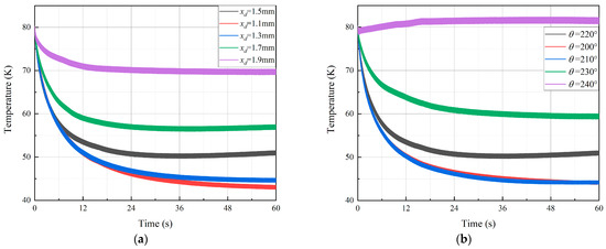
Figure 11.
Cooling curves of ADPTR with different xd and θ: (a) effect of xd on the cooling curve and (b) effect of θ on the cooling curve.
It can be proved from Figure 5 that the cooling performance of ADPTR is significantly improved, especially at lower cooling temperatures. The most commonly used occasions for small low-temperature refrigerators are in the 80 K liquid nitrogen temperature range for refrigeration; therefore, the operating performance of the ADPTR with the variations of xd is compared when the cooling temperature is 80 K in Figure 12, and it will facilitate our analysis of the mechanism of the effect of displacer parameters on the cooling performance of the PTR and provide directions for later optimization. As shown in Figure 12a, the PV power at the displacer is not greatly affected by the change of xd, and the PV power at the compressor is affected as xd gradually increases and reaches a maximum of 64.62 W at xd = 1.7 mm, while the total PV power also reaches a maximum of 70.59 W. The situation also shows that a larger xd is not necessarily conducive to increasing the total input PV power. Figure 12b shows the first increase and then decrease variations of the cooling capacity, COP, and RCOP of the ADPTR with xd, while the red line indicates the COP, and RCOP, which indicates that there is an optimum value of cooling performance with respect to xd. In Figure 12c, the PV power shows a linear increase with the increasing xd, from 7.7 W at xd = 1.1 mm to 10.4 W at xd = 1.9 mm, it but reaches a maximum value of 4.99 W at xd = 1.3 mm and then decreases with increasing xd, resulting in the reduction of FOM from 59.5% to 30.1%, indicating that the larger xd enhances the pushing action of the piston of the displacer, and this, in turn, increases the non-ideal expansion loss in the pulse tube. Figure 12d denotes the detailed losses generated in the regenerator and the pulse tube, from which it can be seen that the non-ideal expansion loss is always larger than the enthalpy flow loss of the regenerator. This is probably due to the fact that the displacer has a much greater effect on the pulse tube than the regenerator.
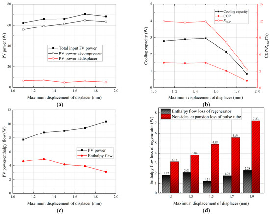
Figure 12.
Operating performance of ADPTR at different xd: (a) PV power; (b) cooling capacity, COP, and RCOP; (c) PV power and enthalpy flow in the pulse tube; and (d) loses in regenerator and pulse tube.
Figure 13 shows the effect of θ on the operating performance of ADPTR when the cooling temperature is 80 K. In Figure 13a, total input PV power, PV power at the compressor, and PV power at the displacer all increase as the θ increases, and the total PV power increases from 51.64 W at θ = 200° to 75.13 W at θ = 230° due to the fact that the lower synchronization rate of the displacer and compressor leads to an increase in the total input PV power. The COP and RCOP keep decreasing as the θ increases in Figure 13b, while the cooling capacity reaches a maximum value of 3.17 W at θ = 210°, lower synchronization rate of displacer and compressor may reduce the cooling performance of the PTR while the red line indicates the COP and RCOP. The PV power of the pulse tube in Figure 13c increases from 5.72 W at θ = 200° to 10.37 W at θ = 230°, but the enthalpy flow is not affected, resulting in a decrease in the pulse tube FOM from 60.23% at θ = 200° to 39.29% at θ = 230°. It can be seen that the synchronization rate of the two pistons has a greater effect on the PV power with a smaller effect on the enthalpy flow in the pulse tube. The detailed losses in the regenerator and pulse tube are shown in Figure 13d, the non-ideal expansion loss is also always larger than the enthalpy flow loss in the regenerator; the changing θ can achieve an effective suppression of the enthalpy flow loss in the regenerator, reaching a minimum value of 0.35 W at θ = 210°.
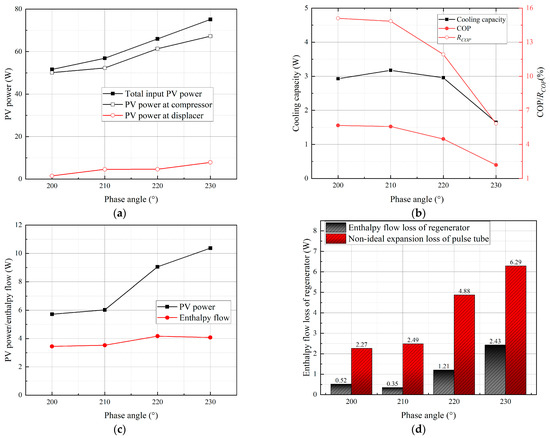
Figure 13.
Operating performance of ADPTR at different θ: (a) PV power; (b) cooling capacity, COP, and RCOP; (c) PV power and enthalpy flow in the pulse tube; and (d) loses in regenerator and pulse tube.
4.2. Kriging Model for ADPTR Optimization
The analysis in Section 4.1 sufficiently demonstrated that xd and θ are essential for enhance the cooling performance of the ADPTR, but the synergistic effect of these two parameters on the cooling performance cannot be derived through a conventional analysis and thus require a more scientific approach. The range of values of xd and θ was locked to 1~2.3 mm and 200°~240°, respectively, and the LHS method was used to randomly choose these two variables; the distribution of 25 samples taken here is shown in Figure 14.
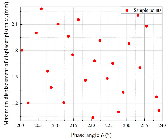
Figure 14.
Distribution of the samples.
CFD simulations were performed for the sample set taken in Figure 14, and the initial temperature fields of both the pulse tube and the regenerator were set with a linear distribution from 80 K to 300 K; i.e., the cold end temperature was cooled down from 80 K, as shown in Figure 11. A Kriging response surface model was constructed based on the two variables and the ADPTR no-load temperature. To verify the prediction accuracy of the Kriging model; Table 2 selected 10 simulated values for comparison with the predicted values, the RMSE of the model was calculated as 1.1, using Equation (25); and the average prediction error percentage is 1.8%, which indicates that the prediction accuracy of the model meets the design requirements for ADPTR.
Table 2.
Comparison results of CFD simulations with predicted values for no-load temperature.
4.3. Discussion on Optimization Results by Genetic Algorithm
In the actual project, the no-load temperature of PTR is the most concerned parameter, and scholars usually take the minimum value of no-load temperature as the optimization target. While optimizing the no-load temperature, other parameters, such as cooling capacity, COP, and input PV power at some specific temperatures, should not be neglected; weighted multi-objective optimization can be performed for these parameters according to the actual demand.
As elucidated in Figure 15a, the response surface of the Kriging model is constructed according to the no-load temperature, and it can be seen that there are obvious maximum and minimum points, and we are more concerned about the minimum point. Taking the minimum value of no-load temperature as the optimization target, the genetic algorithm with Kriging as iterative solver is executed, and then the optimization result is obtained as 35.3 K at xd = 1.24 mm, θ = 206.1°. Taking into consideration the calculation of this combination of variables using CFD simulation results in 39 K, with an error of 3.7 K, which is within the acceptable range, we see that the optimized ADPTR has a 12.1 K reduction in no-load temperature. It is easy to find the optimal combination of the two variables to achieve the minimum no-load temperature by using this method.
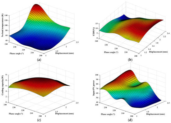
Figure 15.
Distribution of working performance in the sample range: (a) no-load temperature, (b) COP, (c) cooling capacity, and (d) input PV power.
From Figure 15a, we see that, since the no-load temperature of some models in the selected sample space cannot be reduced to a lower level, the operation of ADPTR cooling at 150 K was selected for optimization analysis. The three Kriging models of cooling capacity (Y1), the COP (Y2), and the whole system input PV power (Y3) of the ADPTR were constructed in this sample range to optimize and predict the performance of each ADPTR operation. The response surfaces formed by the three Kriging models are shown in Figure 15b–d, the maximum value of the cooling capacity exists within the sample range, which is known to be 8.86 W, using the Genetic Algorithm solution, corresponding to the combination of the two independent variables, i.e., xd = 1.64 mm and θ = 216.6°, while the other two response parameters have no obvious optimal values but can be used for the design of ADPTR parameters. The prediction accuracy for these three Kriging response surfaces was also verified by using the 10 cases in Table 2, and the comparison results between the simulation results and the model predictions are shown in Table 3. The RMSEs of the three models were 0.15 W, 0.41%, and 2.16 W, respectively, with mean percentage prediction errors of 1.69%, 2.68%, and 2.14%, respectively.
Table 3.
Comparison of simulated and predicted values of three parameters at the cooling temperature of 150 K.
5. Conclusions
In the current study, ITPTR and ADPTR were modeled, and CFD simulations were performed separately to compare the flow and heat transfer characteristics within the cold finger. The optimization and design of displacer parameters for ADPTR was achieved using the Kriging model, and the main results and findings were as follows:
1. Since the displacer allows for the easier adjustment of the phase angle between pressure and mass flow, the ADPTR can achieve a better cooling performance compared to the ITPTR, with a 2.5~3.3 W higher cooling capacity than ITPTR at different temperatures. However, the temperature fluctuations in the pulse tube of ADPTR are more drastic; the velocities and vortex at the hot end are greater, resulting in a lower FOM of pulse tube than ITPTR; and due to the fact that the increase in enthalpy flow of the pulse tube is greater than the increase in non-ideal expansion losses, the ADPTR achieved a higher cooling performance.
2. Both the input PV power and the non-ideal expansion loss in the pulse tube increase with xd, from 7.7 W and 3.14 W at an xd of 1.1 mm to 10.4 W and 7.23 W at an xd of 1.9 mm, respectively. Meanwhile, adjusting the θ can effectively reduce the non-ideal expansion loss in the pulse tube and the enthalpy flow loss in the regenerator, obtaining the minimum value of 0.35 W at θ of 210°. Therefore, a reasonable combination of these two parameters helps us obtain a better cooling performance.
3. The accuracy of the Kriging model in predicting the no-load temperature, cooling capacity, COP, and input PV power is 98.2%, 98.31%, 97.86%, and 97.32%, respectively, which fully meet the design and optimization requirements. In this paper, the minimum value optimization was performed for the no-load temperature, and the optimized temperature is 23.68% lower than the initial one. Depending on the different needs in the actual project, the optimization can also be weighted for multiple objectives.
In summary, although the ADPTR has a more excellent performance than the ITPTR, some components have higher losses during refrigeration due to the operating characteristics of the displacer, so the optimization of key parameters of the displacer is especially important. The genetic algorithm based on the Kriging agent model is a good optimization method, which can also be used to optimize other parameters of PTR with multi-objective optimization according to cooling requirements.
Author Contributions
Writing—review and editing, Z.G.; supervision, W.S., Z.C. and C.Z. All authors have read and agreed to the published version of the manuscript.
Funding
This research was funded by the China Postdoctoral Fund Program (2022M711955), Taishan Scholar Project (tsqn202103142), Youth Fund of Shandong Natural Science Foundation (ZR2021QE182) and Natural Science Foundation of Shandong Province (ZR2020ME192).
Data Availability Statement
Data are contained within the article.
Conflicts of Interest
The authors declare no conflict of interest.
References
- Waele, A.T.A.M. Pulse tube refrigerators: Principle, recent developments, and prospects. Phys. B Condens. Matter 2000, 280, 479–482. [Google Scholar] [CrossRef]
- Ross, R.G. Aerospace Coolers: A 50-Year Quest for Long-Life Cryogenic Cooling in Space. In Book Cryogenic Engineering, 2nd ed.; Timmerhaus, K.D., Reed, R.P., Eds.; Springer: New York, NY, USA, 2007; pp. 225–284. [Google Scholar] [CrossRef]
- Zhang, A.; Wu, Y.; Liu, S.; Yu, H.; Yang, B. Development of Pulse Tube Cryocoolers at SITP for Space Application. J. Low Temp. Phys. 2018, 191, 228–241. [Google Scholar] [CrossRef]
- Gifford, W.E.; Longthworth, R.C. Pulse Tube Refrigeration. Trans. ASME. Eng. Ind. Ser. B 1964, 86, 264–268. [Google Scholar] [CrossRef]
- Mikulin, E.I.; Tarasov, A.A.; Shkrebyonock, M.P. Low-Temperature Expansion Pulse Tubes. Adv. Cryog. Eng. 1984, 29, 629–637. [Google Scholar] [CrossRef]
- Radebaugh, R.; Zimmerman, J.; Smith, D.R.; Louie, B. A comparison of three types of pulse tube refrigerators: New methods for reaching 60 K. Adv. Cryog. Eng. 1986, 31, 779–789. [Google Scholar] [CrossRef]
- Zhu, S.; Wu, P.; Chen, Z. Double inlet pulse tube refrigerators: An important improvement. Cryogenics 1990, 30, 514–520. [Google Scholar] [CrossRef]
- Kanao, K.; Watanabe, N.; Kanazawa, Y. A Miniature Pulse Tube Refrigerator for Temperatures below 100 K. Cryogenics 1994, 34, 167–170. [Google Scholar] [CrossRef]
- Zhu, S.; Nogawa, M. Pulse tube stirling machine with warm gas-driven displacer. Cryogenics 2010, 50, 320–330. [Google Scholar] [CrossRef]
- Wang, X.; Zhang, Y.; Li, H.; Dai, W.; Chen, S.; Lei, G.; Luo, E. A high efficiency hybrid stirling-pulse tube cryocooler. AIP Adv. 2015, 5, 037127. [Google Scholar] [CrossRef]
- Shi, Y.; Zhu, S. Experimental investigation of pulse tube refrigerator with displacer. Int. J. Refrig. 2017, 76, 1–6. [Google Scholar] [CrossRef]
- Abolghasemi, M.A.; Rana, H.; Stone, R.; Dadd, M.; Baileya, P.; Liang, K. Coaxial Stirling pulse tube cryocooler with active displacer. Cryogenics 2020, 111, 103143. [Google Scholar] [CrossRef]
- Rana, H.; Abolghasemi, M.A.; Stone, R.; Dadd, M.; Bailey, P. Numerical modelling of a coaxial Stirling pulse tube cryocooler with an active displacer for space applications. Cryogenics 2020, 106, 103048. [Google Scholar] [CrossRef]
- Xu, J.; Hua, J.; Hu, J.; Zhang, L.; Luo, E.; Gao, B. Experimental study of a cascade pulse tube cryocooler with a displacer. Cryogenics 2018, 95, 69–75. [Google Scholar] [CrossRef]
- Zhu, H.; Jiang, Z.; Liu, S.; Jiang, Y.; Wu, Y. Comparison of three phase shifters for Stirling-type pulse tube cryocoolers operating below 30 K. Int. J. Refrig. 2018, 88, 413–419. [Google Scholar] [CrossRef]
- Pang, X.; Wang, X.; Dai, W.; Li, H.; Wu, Y.; Luo, E. Theoretical and experimental study of a gas-coupled two-stage pulse tube cooler with stepped warm displacer as the phase shifter. Cryogenics 2018, 92, 36–40. [Google Scholar] [CrossRef]
- Liu, B.; Jiang, Z.; Ying, K.; Zhu, H.; Liu, S.; Wen, F.; Wu, Y.; Dong, D. A high efficiency Stirling/pulse tube hybrid cryocooler operating at 35 K/85 K. Cryogenics 2019, 101, 137–140. [Google Scholar] [CrossRef]
- Liu, B.; Jiang, Z.; Ying, K.; Yin, W.; Zhu, H.; Liu, S.; Wu, Y.; Dong, D. Numerical and experimental study on a Stirling/pulse tube hybrid refrigerator operating around 30 K. Int. J. Refrig. 2021, 123, 34–44. [Google Scholar] [CrossRef]
- Abolghasemi, M.A.; Liang, K.; Stone, R.; Dadd, M.; Bailey, P. Stirling pulse tube cryocooler using an active displacer. Cryogenics 2018, 96, 53–61. [Google Scholar] [CrossRef]
- Chen, X.; Ling, F.; Zeng, Y.; Wu, Y. Investigation of the high efficiency pulse tube refrigerator with acoustic power recovery. Appl. Therm. Eng. 2019, 159, 11390. [Google Scholar] [CrossRef]
- Deng, W.; Liu, S.; Chen, X.; Ding, L.; Jiang, Z. A work-recovery pulse tube refrigerator for natural gas liquefaction. Cryogenics 2020, 111, 103170. [Google Scholar] [CrossRef]
- Rout, S.K.; Choudhury, B.K.; Sahoo, R.K.; Sarangi, S.K. Multi-objective parametric optimization of Inertance type pulse tube refrigerator using response surface methodology and non-dominated sorting genetic algorithm. Cryogenics 2014, 62, 71–83. [Google Scholar] [CrossRef]
- Panda, D.; Kumar, M.; Satapathy, A.K.; Sarangi, S.K. Optimal design of thermal performance of an orifice pulse tube Refrigerator. J. Therm. Anal. Calorim. 2021, 143, 3589–3609. [Google Scholar] [CrossRef]
- Wu, W.; Deng, W.; Huang, Y.; Wang, X.; Ji, Y. Prediction of the working conditions for the pulse tube cooler based on artificial neural network model. Appl. Therm. Eng. 2021, 197, 117424. [Google Scholar] [CrossRef]
- Jiang, Z.; Wu, J.; Huang, F.; Lv, Y.; Wan, L. A novel adaptive Kriging method: Time-dependent reliability-based robust design optimization and case study. Comput. Ind. Eng. 2021, 162, 107692. [Google Scholar] [CrossRef]
- Yang, R.J.; Wang, N.; Tho, C.H.; Bobineau, J.P.; Wang, B.P. Metamodeling Development for Vehicle Frontal Impact Simulation. J. Mech. Des. 2005, 127, 1014–1020. [Google Scholar] [CrossRef]
- Prebeg, P.; Zanic, V.; Vazic, B. Application of a surrogate modeling to the ship structural design. Ocean Eng. 2014, 84, 259–272. [Google Scholar] [CrossRef]
- Zheng, C.; Zhao, H.X.; Zhou, Z.Z.; Geng, Z.T.; Cui, Z. Investigation on thermal model updating of Alpha Magnetic Spectrometer inorbit based on Kriging meta-modeling. Nucl. Inst. Methods Phys. Res. A 2022, 1031, 166581. [Google Scholar] [CrossRef]
- Harvey, J. Oscillatory compressible flow and heat transfer in porous media application to cryocooler. Ph.D. Thesis, Georgia Institute of Technology, Atlanta, GA, USA, 2003. [Google Scholar]
- Radebaugh, R. Development of the Pulse Tube Refrigerator as an Efficient and Reliable Cryocooler. In Institute of Refrigeration Proceedings; Institute of Refrigeration: London, UK, 1999. [Google Scholar]
- Chen, L.; Zhang, Y.; Luo, E.; Li, T.; Wei, X. CFD analysis of thermodynamic cycles in a pulse tube refrigerator. Cryogenics 2010, 50, 743–749. [Google Scholar] [CrossRef]
Disclaimer/Publisher’s Note: The statements, opinions and data contained in all publications are solely those of the individual author(s) and contributor(s) and not of MDPI and/or the editor(s). MDPI and/or the editor(s) disclaim responsibility for any injury to people or property resulting from any ideas, methods, instructions or products referred to in the content. |
© 2023 by the authors. Licensee MDPI, Basel, Switzerland. This article is an open access article distributed under the terms and conditions of the Creative Commons Attribution (CC BY) license (https://creativecommons.org/licenses/by/4.0/).