Abstract
Energy retrofit of existing buildings is based on the assessment of the starting performance of the envelope. The procedure for the in situ measurement of thermal conductance is described in the ISO 9869-1:2014, which provides two techniques for data processing: the average method (AM) and the dynamic method (DM). This work studies their effectiveness using virtual data from numerical simulations based on a finite difference model applied to different wall kinds, considering winter and summer boundary conditions alternatively (Italian Milan-Linate TMY). The estimated thermal conductances are compared to the reference theoretical values. The main purposes are: (i) defining the shortest test duration that provides acceptable results; (ii) assess the reliability of the criteria provided by the standard to evaluate the measurement quality; (iii) evaluate the sensitivity of both methods to variables such as wall properties, boundary conditions and others more specific to the DM (namely, the number of time constants and linear equations). The AM always provides acceptable estimates in winter (−3.1% ÷ 10% error), with better outcomes when indoor heat flux is considered, except for the highly insulated wall, but is not effective in summer, despite the fulfillment of the acceptance criteria for the highly insulated wall. The DM provides improvements in both seasons (0.05% ÷ 8.6% absolute values of error), for most virtual samples, and requires shorter sampling periods, even below the 3 days limit suggested by the standard. The test on the confidence interval indicated by the ISO 9869-1:2014 is not reliable and measurements are sensitive to the number of linear equations, that is left to the user’s discretion without strict indications. This work suggests a possible approach for overcoming this issue, which requires deeper future investigation.
1. Introduction
To reduce the energy needs related to the existing building stock, great effort is oriented towards envelope renovation. As a first step in this direction, the thermal properties (thermal transmittance and conductance) of the existing building components are usually assessed through in situ measurements. The scientific literature dedicated to such measurements deals with several techniques, based on various approaches [1,2]. Among all, the so-called heat flow meter (HFM) method is the one implemented by the two main technical standards dedicated to this matter: the American ASTM C1155-95 (2021) [3] and the International ISO 9869-1:2014 [4], which is the subject of this paper. The HFM method consists in monitoring the heat flow density on the surface of the building component, usually on the internal side, together with the indoor and outdoor operative temperatures or surface temperatures, depending on whether the user aims to derive the thermal transmittance or the thermal conductance, respectively.
Going more in detail, the ISO 9869-1:2014 describes two ways of post-processing the data collected in situ, namely the average method (AM) and the dynamic method (DM) and provides several acceptability criteria to evaluate the measurement results. While the AM assumes that measurements are taken when the building component is fundamentally in steady state, the DM is not based on this hypothesis and thus it is potentially more flexible. At the same time, the AM is characterized by a simpler implementation and therefore it is more commonly used [5,6,7].
There are several works within the dedicated literature that investigate these two methods, analyzing some of the key parameters and presenting a wide variety of results. Atsonios et al. [8] investigate the effect measurement conditions and duration have on the quality of the result, showing that the AM is reliable when there is a sufficient temperature difference between indoors and outdoors, while the DM is less sensitive to this parameter. Even though this work studies three different walls, it is not possible to draw conclusions about the influence of the wall construction on the measurement efficacy, since it appears that data acquisition is not performed at the same time for the different walls. The measurement conditions and duration, along with the equipment accuracy, are investigated by Gaspar et al., (2018) [9] to refine the testing procedure for low U-value components, providing useful indications about variables that are not fully specified by the standard, such as the temperature difference, the test duration and the accuracy of the equipment. However, this work focuses only on the AM. The relevance of the temperature difference is also highlighted in the work by Desogus et al. [10], where an increase in experimental uncertainty is observed when the difference between the temperatures of the air at the two sides of the wall is reduced. On the other hand, Lucchi [11] demonstrates the effectiveness of the HFM method, and more precisely the AM, in assessing the thermal properties of stone masonries in historical buildings. Rasooli and Itard [12] aim at mitigating the issues related to the long duration and the precision for measurements to be processed by the AM, suggesting the implementation of an additional external HFM to simultaneously calculate two values for the wall thermal resistance. Their average allows both a reduction in test duration and an improvement in precision. Still focusing on the AM, Evangelisti et al. [13] describe and numerically validate a technique that is successfully applied in a later experimental investigation [14], to filter data, taking into account indoor temperature fluctuations due to heating system working cycles, in order to improve the overall accuracy of the test. An interesting comparison between the AM and DM is presented by Gaspar et al., (2016) in [15], where data are collected for three walls, featuring different U-values, in multiple periods, ranging from early winter to early spring. It is shown that the DM generally provides better results than the AM, especially whenever testing conditions are not optimal (namely, a small indoor-outdoor temperature difference). Moreover, the use of a large data set is generally preferable. The work by Deconinck and Roels [16] is based on data collected through both numerical simulations and experimental measurements and compares the effectiveness of several calculation methods as a function of the test duration and boundary conditions. It shows that, even though semi-stationary methods, such as the AM, provide a performance comparable to the dynamic ones in winter, they handle summer conditions poorly. However, it has to be noticed that the dynamic methods implemented in [10] are not the same as the DM from the ISO 9869-1:2014. A numerical approach is also adopted by Nicoletti et al. [17]: the authors investigate the effectiveness of several methods for in situ measurement of thermal conductance, including the AM and the DM, applied to eight virtual samples of different thickness, thermal resistance and layer sequence. Simulations are performed using measured boundary conditions (indoor and outdoor temperatures, wind velocity) and results proved the reliability of the AM and showed that the DM could be unreliable when abrupt changes in indoor temperature occur. It is however to be noticed that in this work, the effects of solar radiation on the external surface are not considered, in the assumption that the virtual samples are perfectly shielded. In general, works from literature display a significant effort in comparing the effectiveness of different calculation methods [18] and in defining a minimum test duration [19,20] required. According to the review by O’Hegarty et al. [21], the discrepancy between measured and theoretical thermal transmittance increases as the theoretical transmittance decreases. It is also shown that longer test durations tend to provide more reliable outcomes, while the indoor-outdoor temperature difference seems to have a smaller influence.
The literature review has shown that most works deal with the AM, while only few papers investigate the DM, despite its potential interest in practical use. Moreover, these studies have not been paired with: (i) an investigation of the effectiveness of the acceptance criteria provided by the ISO 9869-1:2014 standard and (ii) with a sensitivity analysis to key parameters of the methods (especially for the DM). This kind of information would support technicians in the implementation of these methods in their practice. It is also remarked that, when experimental works are considered, it is generally difficult to relate the effectiveness of the methodologies with the wall typology, as in situ measurements on different walls are hardly performed at the same time and thus are possibly influenced by differences in the occurring boundary conditions.
Therefore, this paper aims to address such open issues, possibly also looking for the shortest reliable test duration as a function of wall properties and boundary conditions, along with supplementary criteria concerning several key parameters involved in each methodology, whose details will be provided with the comprehensive description of the AM and DM in Section 2. To these aims, the average and the dynamic methods are applied to the determination of the thermal property of different wall typologies. To overcome the limitations inherent with experimental approaches, this work adopts virtual wall samples, simulated through a finite difference model, allowing to apply the same controlled and repeatable boundary conditions to building components with different thermal conductances. Moreover, it also allows to exclude the possible effects due to instrumental errors. Therefore, the AM and the DM techniques are applied to data derived from virtual experiments carried out through numerical simulations, rather than from in situ measurements, and results are compared to analytically calculated reference values of the thermal transmittance.
The work presented in this paper is a set of preliminary studies carried out in the context of the VTR BIO SYS project, funded by the Smart Living grant from Regione Lombardia (Italy). The scope of the project was the design of a net zero energy building for emergency use, based on highly insulated dry construction components. The project also included a monitoring phase, aimed at evaluating the overall energy performance of the building.
2. Materials and Methods
In this paper, the average and the dynamic methods of analysis suggested by ISO 9869-1:2014 are applied to virtual data obtained through virtual heat flow meter experiments. The purpose of the data analysis is to derive the “experimental” thermal conductance, that in this case can be compared with the known exact value. In this section, the experimental and data processing approaches by the standard are briefly illustrated. Secondly, the numerical model for heat transfer across the wall is described and the three virtual walls and boundary conditions are provided.
2.1. The HFM Method according to the Standard
The in situ estimation of the thermal conductance is based on the monitoring of the indoor and outdoor surface temperatures (Tsi and Tse, respectively) of a given wall, along with the heat flux density (φ) at one of these surfaces. More precisely, the ISO 9869-1:2014 suggests sampling this quantity at the indoor surface, due to a generally greater stability.
Data processing is then performed according to two possible techniques, the average method (AM) and the dynamic method (DM).
The sampling period is suggested as being at least 72 h if the temperature is stable around the HFM, but it can be longer if required. Moreover, acceptance criteria have to be verified during the course of the test itself. However, this will be discussed later in this work. As far as data acquisition and sampling frequency are concerned, data must be recorded at constant intervals (every 0.5 ÷ 1 h for the AM or with shorter intervals for the DM) and have to be the average of several samples acquired at higher frequency. In this work the sampling frequency is significantly increased, reducing the sampling interval to 5 min to allow for more accurate estimations.
2.1.1. The Average Method
This method is based on the assumption that the conductance can be obtained by dividing the mean heat flux density by the mean temperature difference, both taken over a sufficiently long period of time. According to the AM approach, the overall thermal conductance Λ of the building envelope component is progressively evaluated while the measurement itself is ongoing, through the following equation:
where φi, Tsi,i, and Tse,i are heat flux density [W/m2], indoor and outdoor surface temperature [°C], respectively, at the i-th sampling moment (with i = 1 ÷ N). Both summations in Equation (1) progress with time and their ratio should reach a stable value that approximates the real thermal conductance of the investigated component. According to the standard, results can be generally considered reliable if:
- the heat content of the element is the same at the beginning and at the end of the test (namely, same temperature and moisture distributions);
- the heat flux density is measured in a location not exposed to direct solar radiation;
- thermophysical properties of the materials are constant during the test.
The first condition is hard to assess in real components and the second one largely depends on the date of the measurement and on the location and orientation of the investigated component. Therefore, both are neglected in this work, while the third one is fulfilled due to the hypothesis assumed for the definition of the numerical model, as described later.
This approach is based on the steady state assumption. For this reason, the standard suggests performing the sampling in winter periods, when outdoor conditions are more stable and larger heat flow densities across the walls usually occur. For elements with an expected thermal capacity lower than 20 kJ/(m2K), it is recommended to use only data acquired during the nights. With reference to the total thermal resistance of the construction, defined as R = Λ−1, the standard also provides three conditions that must be fulfilled before ending the test, i.e.,
- the test should last more than 72 h;
- the deviation between the R-value at the end of the test and the value reached 24 h before should be within ±5%;
- the deviation between the R-value obtained considering the first 2/3 and the last 2/3 of the test duration (both rounded at integer) should be within ±5%.
In this work, the constraint on the overall test duration is not strictly considered in order to investigate how much the sampling period can be reduced while maintaining an acceptable outcome of the procedure. At the same time, the other two conditions are always checked. Moreover, the standard suggests either the use of a thermal mass factor correction or the implementation of the DM whenever the change in internal energy of the wall is more than 5% of the heat passing through the wall during the test. Since it is not clearly explained how this condition should be practically assessed and this work deals with the DM anyway, no thermal mass factor correction is considered.
2.1.2. The Dynamic Method
This second processing technique is suggested as a way of estimating the steady-state properties of a building element starting from highly variable temperatures and heat fluxes and is applied at the end of their acquisition. It is based on the solution of the Fourier equation through the Laplace transformation method [22]:
where T’si,i and T’se,i are the surface temperature time derivatives [K/s] at the i-th sampling moment (approximated using the incremental ratio referred to the sampling interval ∆t), K1, K2, Pn and Qn are unknown dynamic characteristics of the wall that depend on the n-th time constant τn (also unknown). Even though the number of time constants should be theoretically infinite, their value rapidly decreases with n and a limited number m (generally from 1 to 3) is adequate to correctly describe the system behaviour. Finally, βn is defined as:
Once the m time constants are initialized, the (2m + 3) unknowns are iteratively calculated, optimizing the τn, through the minimisation of the square deviation between the measured (φi) and the estimated (φ*i) heat flux densities:
The sums over the index j in Equation (2) are the approximation of the integration process and are performed over a supplementary subset of p data, with p = M − N and M the number of data triplets (φi, Tsi,i, and Tse,i) that are actually used in the estimation of Λ, as shown in Figure 1: the two surface temperatures are used to calculate φ*i through Equation (2), while the measured heat flux density is used in Equation (4) during the fitting process.
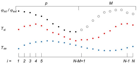
Figure 1.
Representation of the data utilization for the DM, with indication of the subsets of p and M data.
Therefore, the user is expected to choose the number of time constants m, their starting value for the iteration process and M. As far as the time constants are considered, the standard suggests setting m ≤ 3 and defines a ratio r between time constants, usually between 3 and 10, so that:
and for the first time constant the following interval is suggested:
On the other hand, the number M of data triplets used for the estimation of the thermal conductance is left to the user’s experience, providing the only constraint of M > 2m + 3. This means that the resulting set of M linear equations is over-determined. According to the standard 15 to 40 equations should be enough, meaning that 30 to 100 data triplets are needed. However, no univocal criterion is provided to assess the quality of the estimation and, ultimately, of the thermal conductance Λ achieved: the technical standard reports only an equation to calculate the confidence interval I for the estimated Λ, stating that whenever I is lower than 5% of the estimated conductance, the latter is generally close to the real value [4,23].
2.2. The Numerical Model
In this work, virtual experiments are performed using a one-dimensional finite difference (FD) model based on the one presented and validated in [24]. For a given k-th layer of the wall (k = 1 ÷ K), the discretized version of the Fourier equation is:
where αk is the thermal diffusivity, is the temperature at the i-th node (i = 1 ÷ NFD) and at the j-th timestamp (j = 1 ÷ MFD) and ∆x and ∆t are the space and time discretization, respectively. The numerical model uses a central difference scheme for the second order spatial derivative and a fully implicit representation of the time variation (backward Euler).
Third type boundary conditions are considered at both edges of the domain, along with an imposed heat flux at the outdoor surface to take into account solar radiation, while temperature and heat flux continuity is assumed at the interface between adjacent layers. Equations at the edges of each k-th subdomain are derived using the finite volume approach, in order to impose the energy conservations at the interface nodes.
In all simulations performed, a structured grid is considered, with a constant step ∆x = 0.001 m, which in [24] is suggested as a good compromise between accuracy and computational cost, and the timestep ∆t is set equal to 300 s. The model also assumes that materials in the domain are isotropic, homogenous and that their properties do not depend on temperature. As far as air cavities are concerned, their convective heat transfer coefficients are evaluated according to the technical standard ISO 6946:2017 [25], while the radiative component is calculated using the linearization of the heat transfer problem. The intrinsic dependency of these phenomena on the temperatures of the cavity surfaces leads to a non-linear problem, which is solved through an iterative process [26].
The main outcomes of the simulations used by both the AM and the DM are the surface temperature trends, along with the corresponding heat flux densities. For the latter, the three-points formulation is chosen since in [24] it is shown to be a significant improvement over the two-points one:
where φext and φint are the heat flux densities at the outer and the inner edges of the domain, respectively, both positive when directed inward. The algorithm is written in Matlab® and is linked to TRNSYS 18 through an instance of Type 155 (Calling External Program—Matlab), in order to take advantage of the available climate data reading function.
2.3. The Virtual Samples
The effectiveness of the two methods is evaluated on three walls with different thermophysical properties, used as virtual samples: a light and well insulated dry wall (W1—Figure 2a), which is a simplified version of the external walls in the building of the VTR BIO SYS Project; a heavy wall (W2—Figure 2b) that represents historical construction techniques; an externally insulated wall (W3—Figure 2c), which is commonly adopted in new constructions. In this way, it is possible to evaluate the effectiveness of the AM and DM for components with different features. The layer sequences and material thermal properties are reported in Table 1 (density ρ, thermal conductivity Λ, specific heat c and thickness s), along with the following reference quantities, which are calculated according to the equations:
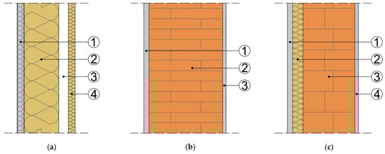
Figure 2.
Layer sequences considered for (a) the light and well insulated dry wall W1, (b) the heavy wall W2 and (c) the externally insulated wall W3. Materials and properties are reported in Table 1.

Table 1.
Names and main properties of the virtual samples. Layer numbering refers to Figure 2.
- thermal conductance
- specific heat capacity per unit area
- time constant
As boundary conditions, two alternative indoor constant values for operative temperatures are considered: 20 °C in winter (from 15 October to 15 April) and 26 °C in summer (the rest of the year). Daily variations are neglected, limiting fluctuations to those caused by the outdoor conditions, which are based on the typical meteorological year for Milan-Linate (Italy). More in detail, both external operative temperature and total solar radiation on a vertical surface facing North are used, in the effort to represent ideal test conditions in terms of orientation, that are aimed at mitigating the confounding effect of incident radiation. Finally, even though the whole year is simulated, only two representative 14-days periods of winter and summer are considered: from the 14 to the 28 of January for winter and from the 1 to the 15 of July for summer (Figure 3).
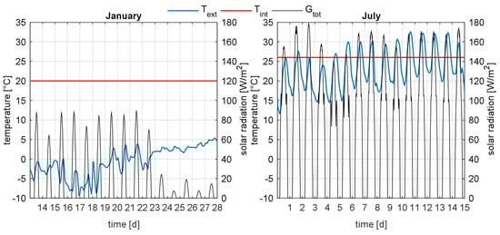
Figure 3.
Indoor and outdoor boundary conditions for the two 14-days periods considered during January and July. For both periods, the red curve represents the indoor operative temperature (Tint), the blue curve represents the outdoor operative temperature (Text) and the black curve represents the total solar irradiation on the horizontal surface (Gtot).
2.4. Data Analysis
As stated above, the main outcomes of the simulations performed on W1, W2 and W3 (namely, the indoor and outdoor surface temperatures and heat flux densities) have been post-processed using either the AM or the DM. Then the estimated thermal conductance has been compared to the reference theoretical value calculated through Equation (10) using the properties reported in Table 1. Since collected data come from a virtual experiment, no instrumental or sampling accuracy has to be taken into account to evaluate the discrepancies between measured and reference thermal conductances. Therefore, since the main source of error might come from the boundary conditions (e.g., temperature stability, indoor-outdoor temperature difference, etc.), discrepancies are considered acceptable if within ±10% [4,23].
As far as the AM is concerned, data calculated for both 14-day periods are fully used: Λ for each virtual sample is estimated through Equation (1), using indoor and outdoor heat flux densities alternatively, starting from the beginning of each period and the outcome of the measurement corresponds to the first time when all requirements from the ISO 9869-1:2014 standard listed in Section 2.1.1 are fulfilled. At the same time, the trends for the estimated thermal conductance are compared to the reference value to verify the reliability of said requirements, along with the overall effectiveness of the AM when related to wall properties and boundary conditions.
Considering the DM, for each wall and each period, sampling windows ranging from one to six days have been investigated. Sampled surface temperatures and heat flux densities are then used in Equations (2) and (4) to estimate the thermal conductance, which is then compared to the reference values. At the same time, the confidence interval I is calculated and its effectiveness in assessing the quality of the measurement procedure is observed. Moreover, the sensitivity of the final outcomes on the number of time constants m and the number of linear equations M is studied parametrically. More in detail, m is varied from 1 to 3, following the indication in the ISO 9869-1:2014 standard, while M goes from a minimum of 6 to a maximum of N-1 with a 10 unit step. Results for winter and summer boundary conditions are presented for each wall only for the shortest time window that provides discrepancies within ±10%.
3. Results
The simulations provide the trends of the surface temperatures and the heat fluxes for each wall, namely the virtual experiment’s data. Results are shown in Figure 4 and also summarised in Table 2 in terms of average, minimum and maximum for every quantity and for both periods considered.
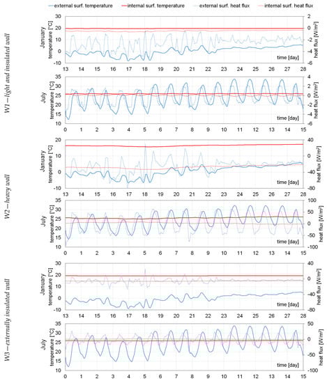
Figure 4.
Simulation results (indoor and outdoor temperature and heat flux density fluctuations) for the three virtual samples investigated.
Table 2.
Average (ave.), minimum (min.) and maximum (max.) indoor and outdoor surface temperatures and heat flux densities for each virtual sample.
During winter, the three walls show stable thermal conditions, with indoor-outdoor temperature differences constant in sign and in all cases above 15 °C on average. Heat flux densities, however, feature higher oscillations on the outer boundaries, with several sign inversions for all walls except W1, likely due to the solar irradiance flux. Indeed, it is important to notice that, even though all virtual samples are oriented toward North, they are not shielded from the diffuse component of solar radiation. On the other hand, a more stable behaviour can be observed on the indoor side, where there are no sign inversions in the heat flux and the absolute values grow with the thermal transmittance of the virtual sample: while for W1 the heat flux density is always below 1 W/m2, for the other two virtual samples, greater absolute values are obtained, with average values above 27 W/m2 and 5 W/m2 for W2 and W3, respectively.
Greater instability can be observed during the summer period, with multiple sign changes for both temperature difference and heat fluxes. Moreover, the average indoor-outdoor temperature difference over the period is below 2 °C for all three walls, while the daily fluctuation of the external surface temperature is consistently in the 10–15 °C range for the whole period in all cases, as shown in Figure 4. This behaviour also affects the heat flux densities that change sign periodically at both indoor and outdoor surfaces, with absolute values that drop with the insulation level of the wall. Even though the observed conditions deviate significantly from the steady state hypothesis and would not be ideal in a real scenario, one of the purposes of this work is to assess the reliability and the robustness of the AM and the DM. Therefore, all the virtual measurements presented are then used to estimate Λ.
3.1. The Average Method
This method has been applied for each wall to the two complete 14-day periods, starting the average process at the beginning of each time window and considering the indoor and outdoor heat flux densities alternatively. Figure 5 shows the conductance curves obtained in both periods for each wall investigated. It is found that the time needed to achieve a reliable estimation is actually the minimum time period required to fulfil the constraints provided by the ISO 9869-1:2014 and reported in Section 2.1.1. The main results for each wall are reported in Table 3, where t is the minimum duration of the test satisfying the constraints by the standard, and n.a. means that for a given condition, even 14-days were not sufficient. It is possible to observe that acceptable outcomes (i.e., up to 10% accuracy) can be achieved for every wall in winter conditions within the minimum 3 days period required by the standard, provided that the proper heat flow density is chosen. In general, while both W2 and W3 feature absolute deviations from the reference below 5%, if the indoor heat flux density is considered and W2 shows an accuracy at the 10% threshold, even when the outdoor one is used for the estimation, for W1 only, φext provides reliable results (i.e., 3.7% error), while φint leads to an unacceptable value of Λ. This is possibly due to the small values of the indoor heat flux density, which is always below 1 W/m2 of absolute value, as a consequence of the high insulation level. This information was also used in the context of the VTR BIO SYS project: since the measurement of the effective walls’ thermal properties is part of the project itself, HFMs have been installed on both internal and external surfaces, to be able to measure both quantities and achieve robust and reliable measurements. Table 3 also shows that increasing the evaluation period up to 14 days does not lead to a significant improvement, as the corresponding estimated conductance Λ14 shows. As an example, in case of W2 and internal heat flux, passing from 3 to 14 days means going from a −3.1% error to a +2% one.
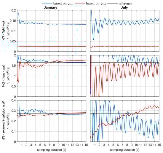
Figure 5.
Outcomes of the AM: progressive estimate of Λ for the three walls in January (left) and July (right), calculated considering the heat flux density either at the outdoor surface (φext—blue curve) or at the indoor surface (φint—red curve) and compared to the known reference value (black curve).
Table 3.
Main outcomes of the AM and the DM for the three virtual samples and the two periods investigated. Results are obtained using the indoor heat flux density (int) or the outdoor heat flux density (ext).
As far as the summer conditions are concerned, the constraints of the standard are never met for W2 and W3, while 5 days are needed for W1. However, despite satisfying the constraints given by the ISO 9869-1:2014, estimations based on the indoor heat flux density lead to an unacceptable value of the thermal conductance (−82% from the reference), while with φext, Λ never stabilizes around an asymptotic value (Figure 5). This oscillatory trend has also been observed when W2 and W3 are considered, wherever the heat flux is measured.
3.2. The Dynamic Method
The DM has been used to process data collected for each of the three walls: several sampling windows inside the two simulation periods considered in this work have been used to assess the efficacy of this methods and to evaluate the shorter time needed to achieve a reliable estimation of the thermal conductance. The first step has been a sensitivity analysis focused on the number of time constants m to be considered in the data processing. Results have shown that this parameter has little to no effect on the final outcomes. Thus, only one time constant τ1 is considered (m = 1) to reduce computational costs. Moreover, results are also independent from the initial value given to this time constant at the beginning of the minimization process of Equation (4). Therefore, the initial value for τ1 has always been set equal to the mean value of the range provided by Equation (6).
For both simulation periods, sampling windows from one to six days have been investigated considering each of the three walls. Figure 6 shows the thermal conductance Λ and the square deviation S2 achieved for both seasons and each virtual sample with the shorter data set needed to achieve acceptable estimations (results are reported as best case in Table 3, and are deemed acceptable if the deviation from reference is within 10%), both as a function of M, namely the number of linear equations considered. Moreover, conductance trends feature the confidence interval, displayed as coloured ranges around the Λ curve, calculated as indicated by the ISO 9869-1:2014.
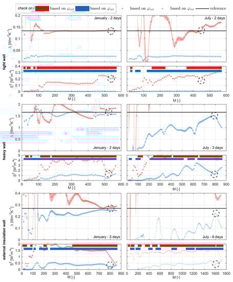
Figure 6.
Outcomes of the DM: estimate of Λ and S2 as function of M for the three walls in January (left) and July (right), considering φext (red dots) and φint (blue dots). The coloured areas around the dotted lines represent the confidence interval I, while the colored horizontal bars indicate when the confidence interval is below the 5% of the estimated Λ.
Outcomes for W1 are similar to those achieved with the AM: despite the better stability, estimations based on φint lead to errors above the 10% threshold, while better agreement (0.05% error) between estimated and reference Λ is obtained using φext. Moreover, if the dependency on M is taken into consideration, winter results are stable for M > 200 (error consistently below 2%), while summer ones show a greater sensitivity on this parameter (error ranging from −48% to +50%). Indeed, even though the true conductance is met in some cases, even small variations in the number of equations to be solved (i.e., ±10) can greatly affect the final outcome and a semblance of stability is only observed in a small range (e.g., see values for M = 350 ÷ 450, where the error ranges from −6% to 7%), leading to difficulty in implementing the DM by the technician. This might be due the greater variability of the boundary conditions during summer days, when daily temperature fluctuations of 10–15 °C at the outdoor surface are observed: different values of M imply different numbers of data triplets involved in the solution of Equations (2) and (4), and such triplets are a direct consequence of the boundary conditions at a given time and their fluctuation can significantly affect the final result. However, in both seasons, two days are enough to achieve acceptable results (Table 3).
As far as W2 is concerned, better outcomes are achieved using the heat flux density at the indoor surface both in January and in July, with a greater stability observable in the winter period (Table 3), when two days of data are enough, and fluctuations are only sporadic and of small entity for M > 300. On the other hand, the summer period needs a three-day data set to provide a result with an error within 10% of the reference Λ (which is still considered acceptable) and is characterized by a trend with a great dependency on the M parameter, which is difficult to interpret.
W3 seems to be the most difficult to investigate among the virtual samples considered in this work: three days of data are needed in winter to achieve an acceptable result, for both indoor and outdoor heat flux densities, and most of the data triplets are used to solve Equation (2) (M > 700), while in summer several time frames have been considered (1 to 14 days) without success (the six-day one is shown in Figure 6 as an example). Finally, for each wall and both seasons, the S2 trend as a function of M is reported below the Λ one and coloured horizontal bars are reported where the confidence interval is within 5% of the estimated thermal conductance. It is possible to observe that this test, suggested by the ISO 9869-1:2014 standard, would deem as acceptable outcomes those that are far from the reference value: as an example, for W3 summer measurements, if φint is considered for calculations, when M ranges from 1100 to 1200, the estimated Λ should be accepted according to the test on I, while the actual errors are between 100% and 120%.
4. Discussion
Results related to the AM show that the indications provided by the standard are only partially effective: even though for W2 and W3 the fulfilment of the conditions described in Section 2.1.1 in the winter measurements generally leads to estimated thermal conductances characterized by a deviation from the reference within the 10% threshold (with the only exception of the 13.1% error for W3 when φext is used for calculations) and is not achieved during the summer period, when Λ is not converging to a stable value, this set of tests appears unreliable when W1 is investigated. Indeed, for this virtual sample, constrains are met in both periods and for both heat flux densities, but do not correspond to acceptable estimations (namely, when φint is used, the absolute value of the error is above 80% and the measured thermal conductance is significantly underestimated), nor reflect a convergence of Λ toward a stable value (as observed for summer measurements with φext). Therefore, conditions suggested by the ISO 9869-1:2014 are not sufficient when highly insulated walls are investigated (Λref = 0.134 W/(m2K) for W1). Moreover, it is important to notice that the constraints in the standard only consider the apparent stability of the thermal conductance estimate by sampling it at the specific moment of the measurement process that are multiples of 24 h, and do not allow to portray the overall trend or to assess the plausibility of the final outcome. Thus, the calculations required by the standard need to be supported by a critical evaluation of the results and a visual inspection of the thermal conductance trend during the whole sampling period.
At the same time, results presented in Section 3.1 show that, when the heat flux density is measured at the indoor surface of the wall, the AM becomes less effective with increasingly insulated constructions. This finding confirms the trend reported in the review presented by O’Hegarty et al. [21] and the numerical outcomes achieved by Nicoletti et al. [17]. Results suggest that a stable heat flux is not enough to achieve a reliable estimate of the thermal conductance, but its absolute value needs to be above a threshold (even the −6 to −4 W/m2 observed for W3 seem to suffice). If highly insulated walls such as W1 are investigated, it has been observed that, even when the sign of the indoor-outdoor temperature difference is constant during the whole sampling period such as in winter, more reliable outcomes are achieved when φext is used, despite the presence of solar radiation. However, even though reference thermal conductances in [17] are of the same order of magnitude as those of W2 and W3 (no work from literature has been found where walls with Λ similar to that of W1 are studied), it is important to notice that a direct comparison of results is unpractical, since the boundary conditions are significantly different. For similar reasons, a direct comparison to experimental studies [5,6,7,14] would not be conclusive, since they are affected by the sensors’ accuracy.
Finally, results confirm that the difficult boundary conditions typical for the summer season do not allow reliable measurements, as shown in [17], even when a long two-weeks sampling period is considered, and that the AM is better suited for winter conditions.
Even though the DM, according to the ISO 9869-1:2014, should be more effective than the AM when dealing with variable indoor and outdoor temperatures, results show that it provides better outcomes with the stable boundary conditions, constant direction of the heat flux (namely, constant sign of the indoor-outdoor temperature difference) and low solar radiation observed for the winter period. Therefore, even though this method is potentially able to deal with the large temperature and heat flux density fluctuations registered in summer, winter periods are to be preferred for data collection. This finding confirms the results presented by Gaspar et al. [15] and by Nicoletti et al. [17]. Moreover, Figure 6 shows that the confidence interval calculated according to the standard does not provide any meaningful indication to the technician to assess the reliability of the estimated Λ: the fulfilment of the criterion “I < 5% of the estimated Λ”, shown in Figure 6 as horizontal coloured bars in the S2 graphs, occurs for many values of M, even when the discrepancy between reference and estimated thermal conductance is unacceptable (>10%).
Moreover, results show that the number of equations that should be sufficient according to the standard (i.e., 15 to 40) is not adequate in any of the cases considered, and this indication should not be taken into account when choosing the value for M.
In general, the interpretation of the outcomes of each analysis based on the DM is not straightforward: the sensitivity to M is great in several cases and the lack of effective indications by the ISO 9869-1:2014 on how to define this parameter and how to assess the quality of the final outcome may be an issue in the implementation of this method in a real context, since the reference thermal conductance to validate the estimations is usually unknown. Additionally, the post-fitting value of the time constant does not provide any indication about the reliability of the results: τ1 in the best conductance estimates shown in Table 3 (grouped under best case) differs significantly from the respective reference τref, calculated using Equation (10) and based on the lumped capacity, suggesting that it is not possible to assign this physical meaning to τ1 and use it as a guidance.
Therefore, to process a given dataset with the DM, the technician has to set the M parameter, without being supported by guidelines from the standard. The parametrical studies performed in this work show that to identify an accurate estimate of Λ, a possible indication might come from the S2 trend as a function of M: good outcomes are indeed achieved for values of M greater than N/2 and corresponding to the last local minimum of S2 (highlighted by dashed circles in Figure 6 and grouped in Table 3 as S2 loc min). This behaviour has been observed in several other cases, when different time frames have been considered. Hence, it suggests that a technician should perform a sensitivity analysis on M and evaluate the outcomes using the S2 trend as described above. Even though better approximations of Λ might be found at different values of M, those conditions either happen when outcomes of the DM experience large fluctuations for small variations of M (namely, when the number of equations is significantly smaller than N/2) or are not identifiable through any proxy variable.
The repeatability of this empirical observation has been tested on two additional virtual samples (A and B), adopting the following approach that simulates a blind test: first of all, two different layer sequences have been defined, without knowing in advance their thermal conductances, and the resulting walls have been simulated using the same boundary conditions presented in Section 2.3. Then, the estimation of their Λ values have been performed parametrically, such as what has been carried out for W1, W2 and W3, but in two steps of increasing refinement. In the first step, M has been varied by a value of 10 each time, and the local minimum of the S2 curve described above, along with the corresponding M (namely, Mst1), has been found through a dedicated automatic search algorithm. The second step consists of a second iteration of the same parametric analysis, focusing the investigation on the range M = Mst1 ± 10, solving Equation (2) for every value in this interval and looking once again for the new and more precise local minimum of the S2 curve, that should correspond to an acceptable estimate of the thermal conductance, according to the hypothesis under investigation. This process has been repeated 20 times for each of the two walls, considering random sampling periods taken from the whole simulation year and with a length, also randomly determined, in the range of 2 to 5 days. At this stage, calculations have only been performed considering the indoor heat flux density. Only as a final step, the true thermal conductances of these virtual samples have been calculated and used as a reference (0.237 W/(m2K) for wall A and 2.763 W/(m2K) for wall B). Results are summarized in the top part of Figure 7.
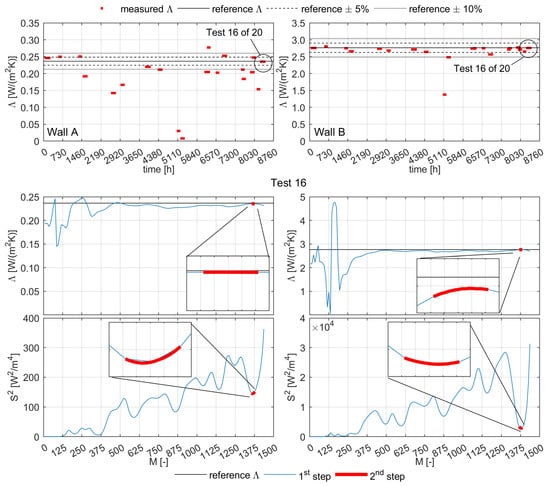
Figure 7.
Evaluation of the research algorithm to define a suitable M value. Result of all the sampling periods tested (red dots) for both walls (the externally insulated A on the left, the heavy and non-insulated B on the right) are shown on the top and compared to the reference value (continuous black line), and to the ±5% (dashed lines) and the ±10% (grey lines) error ranges. An example of the search process is shown on the bottom (sampling period 16 of 20). The evolution of the estimated Λ and the corresponding S2 are reported for the first step (blue curve) and the second step (red curve) of calculation. Thermal conductances are compared to the reference value (black line).
The effectiveness of this search process has then been verified, inspecting each Λ and S2 trend as a function of M and comparing the former to the reference, as shown as an example in the bottom part of Figure 7. This analysis has shown a generally good reliability of this technique, which is able to locate acceptable thermal conductance estimations among those calculated at different M values. This is especially valid for the wall B, which can be brought back to the typology if the heavy wall (W2), for which 19 out of 20 applications of this criterion lead to estimate Λ with less than 10% error (Figure 7). On the contrary, applying this criterion to wall A, which can be brought back to the typology of the externally insulated wall (W3), leads to an acceptable estimate of the conductance in 9 out of 20 applications. As it was remarked previously, the latter wall typology seems particularly difficult to analyse with the DM.
Thus, this approach could support technicians in the application of the DM to in situ measurements, by allowing them to define an effective number of linear equations to solve in the algorithm. However, it is not able to provide any indication of the discrepancy between the final Λ estimated and its correct value. Yet, it is the opinion of the authors that this method should be tested further on different wall samples, and considering different boundary conditions (namely, different weather data and different orientations), and that a physical explanation should be investigated.
5. Conclusions
This work investigates the accuracy of the post processing techniques provided by the ISO 9869-1:2014 by means of numerical simulations on three virtual wall samples subjected to Milan-Linate (Italy) boundary conditions and focuses on two 14-day periods in January and July. The aim of this study was to evaluate the efficacy of these methods in estimating the thermal conductance of constructions with different insulation levels (theoretical thermal conductance going from 0.134 W/(m2K) to 1.661 W/(m2K)) during different seasons, and the effort was focused on assessing the dependency of the outcome on parameters specific to each method, such as: the shortest reliable test duration for both AM and DM, the number of time constants and linear equations solved for the DM.
Results for the AM show that:
- Winter is the best period to implement this, since boundary conditions are more stable (namely, the indoor-outdoor temperature difference keeps a constant sign during the whole period) and differences between measured and reference thermal transmittance can be kept below the ±10% threshold.
- Summer measurements do not allow to achieve any meaningful outcome, even when considering long sampling periods (up to 14 days).
- For highly insulated walls (Λref = 0.134 W/(m2K) in this work), an outdoor heat flux density measurement should be performed on the outer surface, rather than the inner one suggested by the technical standard. Under the conditions investigated in this work (North orientation not shielded from solar radiation, winter measurement), it has been observed that a sufficient amplitude (above 1 W/m2) of the heat flux density is needed to reduce the absolute value of the error (going from 82% with φint to 2% with φext).
- Measurements on the light and highly insulated wall show that the acceptance criteria included in the standard can be misleading, since it tests the stability of the measurement only at 24 h intervals and, therefore, it is not able to assess the actual stability of the measurement trend and does not guarantee the accuracy of the outcome. Thus, technicians should carefully analyse the conductance trend over time to verify convergence to a stable value, which has to be critically evaluated.
As far as the DM is concerned, it was found that:
- For winter measurements, this method requires shorter sampling durations than the AM (going from 2 to 3 days for the light and insulated wall and for the heavy one), leading to errors with absolute values in the range between 0.2% and 4.2%.
- In some cases, this method is able to handle summer conditions (−0.5% error with the light and highly insulated wall using φext, −8.6% error with the heavy wall using φint).
- For the light and highly insulated wall, the outdoor heat flux density measurement should be preferred to the indoor one, as observed with the AM.
- Under the conditions tested in this work, increasing the number of time constants does not lead to any improvement to the final outcomes, and the value of this quantity at the end of the fitting process is not comparable to the time constant calculated using the lumped parameter approach (τref).
- Great sensitivity on the number of interpolated equations M is observed, especially when dealing with summer measurements, and the confidence interval calculated according to the standard does not reliably indicate the quality of the outcome, making the DM difficult to implement and the results hard to interpret when the method is applied to a wall with unknown properties.
To solve this issue, a promising correspondence between an acceptable thermal conductance value (error below the ±10% threshold) and the local minimum of the S2 for M near to N was found. This observation has been tested on two new walls by applying a dedicated automatic search algorithm to several sampling periods randomly chosen over a one-year simulation. Findings suggest that, instead of defining a fixed and arbitrary value for M, a technician should perform a parametric analysis over this quantity when applying the DM to a set of data triplets and use the resulting S2 trend to choose the suitable M, thus reaching the final estimated thermal conductance. This approach seems to be more effective for the heavy walls than for the externally insulated ones. However, more studies will be performed in future, to extend the number of virtual samples tested and to provide a theoretical explanation.
Finally, it was found that both AM and DM are sensitive to the wall typology. Therefore, estimating the kind of wall in advance is key to acquiring the heat flow signal on the most suitable side.
Since in this work, only few walls are investigated and only Milan-Linate (Italy) weather data are considered in simulations, future efforts will be dedicated to extending the number of virtual samples considered and performing numerical simulations with different boundary conditions. Moreover, future works will also be dedicated to defining and testing procedures to provide the technicians support in assessing the quality of the measurement, when either the AM or the DM is implemented.
Author Contributions
Conceptualization, A.A. (Andrea Alongi), A.A. (Adriana Angelotti) and L.M.; methodology, A.A. (Andrea Alongi) and A.A. (Adriana Angelotti); software, A.A. (Andrea Alongi) and L.S.; validation, A.A. (Andrea Alongi) and L.S.; formal analysis, A.A. (Andrea Alongi) and A.A. (Adriana Angelotti); data curation, A.A. (Andrea Alongi); writing—original draft preparation, A.A. (Andrea Alongi); writing—review and editing, A.A. (Andrea Alongi) and A.A. (Adriana Angelotti); visualization, A.A. (Andrea Alongi); supervision, A.A. (Adriana Angelotti) and L.M.; project administration, L.M.; funding acquisition, L.M. All authors have read and agreed to the published version of the manuscript.
Funding
This research was funded by Lombardy Region, Smart Living grant “SMART VTR BIO SYS”.
Data Availability Statement
Not applicable.
Conflicts of Interest
The authors declare no conflict of interest.
Abbreviations
| AM | average method |
| DM | dynamic method |
| FD | finite difference model |
| HFM | heat flow meter |
| W1, W2, W3 | virtual wall samples |
| Nomenclature | |
| C | specific heat capacity per unit area [kJ/(m2K)] |
| c | specific heat capacity [J/(kgK)] |
| Gtot | total solar irradiation on the horizontal surface [W/m2] |
| I | confidence interval [-] |
| i, j, k | index [-] |
| K1, K2 | unknown dynamic characteristics of the wall [J/(m2K)] |
| M | number of linear equations [-] |
| m | number of time constants [-] |
| N | number of data sampled [-] |
| Pn, Qn | unknown dynamic characteristics of the wall [W/(m2K)] |
| p | supplementary data subset [-] |
| R | thermal resistance [m2K/W] |
| r | ratio between time constants [-] |
| S2 | heat flux density square deviation [W2/m4] |
| s | layer thickness [m] |
| T | temperature [°C] |
| T′ | temperature time derivative [°C/s] |
| t | time coordinate [s] |
| x | space coordinate [m] |
| Greek Letters | |
| α | thermal diffusivity [m2/s] |
| βn | exponential function of the time constant [-] |
| Λ | thermal conductance [W/(m2K)] |
| Λ | thermal conductivity [W/(m∙K)] |
| ρ | density [kg/m3] |
| τ | time constant [s]/characteristic time [d] |
| φ | heat flux density [m2] |
| Subscript | |
| cav | cavity |
| cd | conductive |
| ext | quantity referred to outdoor |
| int | quantity referred to indoor |
| ref | reverence value of a quantity |
| se | quantity referred to outdoor surface |
| si | quantity referred to indoor surface |
References
- Teni, M.; Krstic, H.; Kosinski, P. Review and comparison of current experimental approaches for in-situ measurements of building walls thermal transmittance. Energy Build. 2019, 203, 109417. [Google Scholar] [CrossRef]
- Bienvenido-Huertas, D.; Moyano, J.; Marín, D.; Fresco-Contreras, R. Review of in situ methods for assessing the thermal transmittance of walls. Renew. Sustain. Energy Rev. 2019, 102, 356–371. [Google Scholar] [CrossRef]
- ASTM C1155-95 (2021); Standard Practice for Determining Thermal Resistance of Building Envelope Components from the In-Situ Data. ASTM International: West Conshohocken, PA, USA, 2021.
- ISO 9869-1:2014; Thermal Insulation—Building Elements—In-Situ Measurement of Thermal Resistance and Thermal Transmittance—Part 1: Heat Flow Meter Method. International Standard: Geneva, Switzerland, 2014.
- Cabeza, L.F.; Castell, A.; Medrano, M.; Martorel, I.; Pérez, G.; Fernandez, I. Experimental study on the performance of insulation materials in Mediterranean construction. Energy Build. 2010, 43, 630–636. [Google Scholar] [CrossRef]
- Asdrubali, F.; D’Alessandro, F.; Baldinelli, G.; Bianchi, F. Evaluating in situ thermal transmittance of green buildings masonries—A case study. Case Stud. Constr. Mater. 2014, 1, 53–59. [Google Scholar] [CrossRef]
- Ficco, G.; Iannetta, F.; Ianniello, E.; d’Ambriosio Alfano, F.R.; Dell’Isola, M. U-value in situ measurement for energy diagnosis of existing buildings. Energy Build. 2015, 104, 108–121. [Google Scholar] [CrossRef]
- Atsonios, I.A.; Mandilaras, I.D.; Kontogeorgos, D.A.; Founti, M.A. A comparative assessment of the standardized methods for the in-situ measurement of the thermal resistance of building walls. Energy Build. 2017, 154, 198–206. [Google Scholar] [CrossRef]
- Gaspar, K.; Casals, M.; Gangolells, M. In situ measurement of façades with a low U-value: Avoiding deviations. Energy Build. 2018, 170, 61–73. [Google Scholar] [CrossRef]
- Desogus, G.; Mura, S.; Ricciu, R. Comparing different approaches to in situ measurement of building components thermal resistance. Energy Build. 2011, 43, 2613–2620. [Google Scholar] [CrossRef]
- Lucchi, E. Thermal transmittance of historical stone masonries: A comparison among standard, calculated and measured data. Energy Build. 2017, 151, 393–405. [Google Scholar] [CrossRef]
- Rasooli, A.; Itard, L. In-situ characterization of walls’ thermal resistance: An extension to the ISO 9869 standard method. Energy Build. 2018, 179, 374–383. [Google Scholar] [CrossRef]
- Evangelisti, L.; Guattari, C.; Asdrubali, F. Influence of heating systems on thermal transmittance evaluations: Simulations, experimental measurements and data post-processing. Energy Build. 2018, 168, 180–190. [Google Scholar] [CrossRef]
- Evangelisti, L.; Guattari, C.; De Lieto Vollaro, R.; Asdrubali, F. A methodological approach for heat-flow meter data post-processing under different climatic conditions and wall orientations. Energy Build. 2020, 223, 110216. [Google Scholar] [CrossRef]
- Gaspar, K.; Casals, M.; Gangolells, M. A comparison of standardized calculation methods for in situ measurements of façades U-value. Energy Build. 2016, 130, 592–599. [Google Scholar] [CrossRef]
- Deconinck, A.; Roles, S. Comparison of characterization methods determining the thermal resistance of building components from onsite measurements. Energy Build. 2016, 130, 309–320. [Google Scholar] [CrossRef]
- Nicoletti, F.; Cucumo, M.A.; Arcuri, N. Evaluating the accuracy of in-situ methods for measuring wall thermal conductance: A comparative numerical study. Energy Build. 2023, 290, 113095. [Google Scholar] [CrossRef]
- Larsen, S.F.; Hongn, M.; Castro, N.; González, S. Comparison of four in-situ methods for the determination of walls thermal resistance in free-running buildings with alternating heat flux in different seasons. Constr. Build. Mater. 2019, 224, 455–473. [Google Scholar] [CrossRef]
- Gaspar, K.; Casals, M.; Gangolells, M. Review of criteria for determining HFM minimum test duration. Energy Build. 2018, 176, 360–370. [Google Scholar] [CrossRef]
- Choi, D.S.; Ko, M.J. Analysis of Convergence Characteristics of Average Method Regulated by ISO 9869-1 for Evaluating In Situ Thermal Resistance and Thermal Transmittance of Opaque Exterior Walls. Energies 2019, 12, 1989. [Google Scholar] [CrossRef]
- O’Hegarty, R.; Kinnane, O.; Lennon, D.; Colclough, S. In-situ U-value monitoring of highly insulated building envelopes: Review and experimental investigation. Energy Build. 2021, 252, 111447. [Google Scholar] [CrossRef]
- Ahvenainen, S.; Kokko, E.; Aittomaki, A. Thermal Conductance of Wall-Structures—Report 54; Technical Research Centre of Finland, Laboratory of Heating and Ventilating: Espoo, Finland, 1980. [Google Scholar]
- Roulet, C.; Gass, J.; Markus, I. In-situ U-value measurement: Reliable results in shorter time by dynamic interpretation of measured data. In Proceedings of the 3rd Thermal Performance of the Exterior Envelopes of Building Conference, Clearwater Beach, FL, USA, 2–5 December 1985. [Google Scholar]
- Alongi, A.; Angelotti, A.; Mazzarella, L. A numerical model to simulate the dynamic performance of Breathing Walls. J. Build. Perform. Simul. 2021, 14, 155–180. [Google Scholar] [CrossRef]
- ISO 6946:2017; Building Components and Building Elements—Thermal Resistance and Thermal Transmittance—Calculation Methods. International Standard: Geneva, Switzerland, 2016.
- Alongi, A.; Angelotti, A.; Mazzarella, L. Investigating the control strategies for Breathing Walls during summer: A dynamic simulation study. In Proceedings of the 17th IBPSA Conference, Bruges, Belgium, 1–3 September 2021; pp. 261–268. [Google Scholar]
Disclaimer/Publisher’s Note: The statements, opinions and data contained in all publications are solely those of the individual author(s) and contributor(s) and not of MDPI and/or the editor(s). MDPI and/or the editor(s) disclaim responsibility for any injury to people or property resulting from any ideas, methods, instructions or products referred to in the content. |
© 2023 by the authors. Licensee MDPI, Basel, Switzerland. This article is an open access article distributed under the terms and conditions of the Creative Commons Attribution (CC BY) license (https://creativecommons.org/licenses/by/4.0/).