Application of Deep Neural Network in Gearbox Compound Fault Diagnosis

Abstract

Gearbox fault diagnosis is vital to ensure the efficient operation of rotating machinery, and most gearbox faults in industrial production occur in the form of compound faults. To realize the diagnosis of compound faults in gearboxes at different speeds, an “end-to-end” intelligent diagnosis method based on an efficient channel attention capsule network (ECA-CN) is proposed. First, the process uses a deep convolutional neural network to extract fault features from the collected raw vibration signals, embeds the efficient channel attention module to filter important fault features, uses the capsule network to vectorize the feature space information and, finally, calculates the correlation between different levels of capsules using a dynamic routing algorithm to achieve accurate gearbox compound fault diagnosis. The effectiveness of the proposed ECA-CN fault diagnosis method is verified using the composite fault dataset of the 2009 PHM Challenge gearbox, with an average accuracy of 99.63 ± 0.22%. In the comparison experiments using the traditional fault diagnosis method, the average accuracy of the ECA-CN method improved by 4.62%, and the standard deviation was reduced by 0.58%. The experimental results show that the ECA-CN has a more competitive diagnostic performance than traditional shallow machine learning models and CNNs.

1. Introduction

Gearboxes are one of the most widely used speed and power transfer elements in rotating machinery and play a vital role in manufacturing. Gearboxes contain gears, rolling bearings, drive shafts, and other components, which usually operate under harsh operating conditions with different speeds and loads and are prone to failures. In addition, gearbox failure may lead to unexpected downtime, causing substantial economic losses and significant casualties. Therefore, it is essential to study gearbox fault diagnosis to ensure the efficient operation of mechanical systems [1].

Generally speaking, gears and bearings are the two components in gearboxes that are most prone to failure. Common failures include broken teeth, tooth surface wear, bearing fatigue spalling, and running wear [2]. In addition, the loss of one component often causes the failure of another element in contact with it, triggering a compound failure. In the practical application of gearboxes, the features of solid faults easily cover the information of weak fault features due to the different damage mechanisms and loss degrees of individual defects embedded in the vibration signals [3]. Together with the complex transmission path of the movement, the vibration effects generated by different faults will interact, making the coupling and modulation phenomenon between the signals more severe and the mark features challenging to extract.

Traditional composite fault diagnosis methods usually use signal processing techniques, such as wavelet transform analysis [4], envelope analysis [5], and empirical modal decomposition [6,7], for feature extraction and then shallow machine learning models, such as BP neural networks [8] and support vector machines [9], for fault classification. Although traditional methods have achieved fruitful results, the following drawbacks still exist in the era of big data [10]: (1) the process of feature extraction and selection using signal processing techniques is complex, requires manual operations, and relies mainly on engineering experience; (2) manual feature extraction reduces the complexity of the input data and causes rich fault state information to be lost in the original data; and (3) the traditional signal feature extraction techniques make it difficult to separate the coupled features of compound faults.

Deep learning has been widely used in fault diagnosis and is driven by artificial intelligence technology in recent years. Compared with traditional methods of diagnosis, deep-learning-based fault diagnosis methods are free from the reliance on expert knowledge and signal preprocessing methods, can directly excavate the composite fault features hidden in the original vibration signal, and have obvious advantages in the face of massive data. The main classical intelligent diagnosis models are self-encoder [11], recurrent neural network [12,13], convolutional neural network [14], etc. The convolutional neural network (CNN) is the most widely used among them. This is due to the fact of its features, such as local connectivity, weight sharing, and pooling operations, which can effectively reduce the number of training parameters, have strong robustness, and are easy to train and optimize. Yao et al. [15] proposed a CNN-based composite fault diagnosis method that converts bearing vibration signals into grayscale maps as training samples for the network, which can effectively identify bearing hybrid faults in urban rail trains. Zhang et al. [16] considered a deep convolutional generative adversarial network model in the case of insufficient diagnostic samples and effectively improved the composite fault diagnosis by generating additional composite fault data samples. Sun et al. [17] combined an improved particle swarm optimized variational modal decomposition with a CNN to achieve the mixed fault diagnosis of planetary gearboxes. Although the above methods achieved good results, each channel contains different information learned by the convolutional kernel for the features extracted by CNN. The traditional CNN gives the same weight to each track, ignoring the importance of the elements contained in different channels for the fault diagnosis task.

The attention mechanism considers the weight effect (i.e., the mapping relationship between input and output), which can enhance the key features and weaken the redundant components [18,19]. Therefore, introducing the attention mechanism into the diagnostic model can improve the effectiveness and reliability of the method. Li et al. [20] designed a fusion strategy based on the channel attention mechanism to obtain more fault-related information when fusing multisensor data features. Xie et al. [21] constructed an improved CNN incorporating the channel attention mechanism for the fault diagnosis of diesel engine systems. The model mentioned above, considering feature weights, achieves good results, but scalar neurons reduce specific parameters, such as location and scale, in the feature mapping of their subject network CNN. Therefore, the fully connected layer requires a large amount of data to estimate the parameters of the features, and the demand for memory, computation, and data is enormous [22]. On the other hand, the pooling layer of the CNN gives the model a prior probability that is not affected by the translation but loses specific spatial information. In other words, CNNs obtain invariance rather than covariance [23].

In 2017, Sabour et al. [23] proposed a capsule neural network that uses vectors to describe the object representation, where each set of neurons forms a capsule, and the capsule layer outputs vectors, with the vector length indicating the probability of the object presentation; the vector’s direction means the instantiation parameter. In mechanical fault diagnosis applications, multidimensional capsules can retain specific feature parameters at different rotational speeds. In addition, the capsule’s distance represents the features’ dispersion, so the capsule network’s classification quality is better than traditional neural networks. Zhang et al. [24] combined wavelet transform and capsule network for bearing fault diagnosis in high-speed trains. Ke et al. [25] proposed an improved capsule network for the problem of insignificant composite fault features in modular multilevel converters.

Although these methods achieved good results, the feature weights in the feature extraction process were not considered, and the key features were given the same consequences as the redundant features. In addition, the research on compound fault diagnosis is only on diagnosing compound faults occurring in a single component. In contrast, in actual production, compound faults are usually coupled by multiple component faults in the transmission system. Therefore, an efficient channel attention capsule network is proposed for the problem of multicomponent composite fault diagnosis in gearbox drive systems at different speeds. This method uses a one-dimensional convolutional neural network to extract composite fault features, introduces an efficient channel attention module to assign weights to the channel features, and performs composite fault classification using the capsule network.

The main contributions of this paper are as follows: (1) The ECA-CN discards the pooling layer in the traditional CNN and introduces a capsule network instead, using a dynamic routing algorithm instead of a pooling operation to ensure that the core features are not lost. (2) The activation function of the ECA-CN is selected using GELU instead of the commonly used ReLU, and an efficient channel attention module is introduced to provide weights for the features and focus the attention of the network on the key fault features, thus accelerating the convergence of the network and effectively improving the robustness of the model. (3) This method does not require a time-consuming manual feature extraction process and can achieve end-to-end gearbox composite fault diagnosis at different speeds.

This paper is organized as follows: Section 2 details the relevant theories, such as one-dimensional convolution, capsule networks, and marginal loss functions. Section 3 presents the proposed method. In Section 4, the effectiveness and superiority of this paper’s process are verified using the gearbox dataset of PHM2009. Section 5 summarizes this paper’s research conclusions and the outlook for future research work.

2. Related Theory

2.1. One-Dimensional Convolution

In fault diagnosis, since the fault data are a one-dimensional vibrating signal, feature extraction is mainly performed using one-dimensional convolution. The role of the convolution layer is to convolve the local receptive domain of the input signal with the convolution kernel. Each convolution kernel extracts the local features of the input signal’s local receiver domain under the activation function’s action to construct the output feature vector. The output feature vector of each layer is the result of the convolution of multiple input features. The computational equation is as follows:

$$y_i^{l+1}\left(j\right)=K_i^l\ast x^l\left(j\right)+b_i^l$$

(1)

$$a_i^{l+1}\left(j\right)=f\left\{y_i^{l+1}\left(j\right)\right\}$$

(2)

where $x^l$ is the input signal of the $l$th layer; $K_i^l$ is the weight matrix of the $i$th convolution kernel of the $l$th layer; $b_i^l$ is the bias; $y_i^{l+1}$ is the eigenvalue extracted from the $i$th convolution kernel of the $l$th layer; $f\left\{\cdot \right\}$ denotes the activation function; and $a_i^{l+1}\left(j\right)$ denotes the $i$th element of the output eigenvector of the $l$th layer.

The activation function enables the network to obtain the capability of nonlinear representation, enhance the feature representation of the model, map the initially linear and indistinguishable multidimensional features to another space, and make the features learned by the network more distinguishable. In recent years, the rectified linear unit (ReLU) has been widely used as the activation function of the fault diagnosis model to accelerate the convergence of the model, and its calculation formula is as follows:

$$f\left(x\right)=\max \left(0,x\right)$$

(3)

This paper used the Gaussian error linear unit (GELU) [26], calculated as follows:

$$f\left(x\right)=xP\left(X\le x\right)=x\Phi \left(x\right)$$

(4)

$$\Phi \left(x\right)=x{\displaystyle {\int }_{-\infty }^x\frac{e^{-\frac{{\left(X-\mu \right)}^2}{2{\sigma }^2}}}{\sqrt{2\pi }\sigma }}dx$$

(5)

where $x$ denotes the activation value input of the current neuron, and $\Phi \left(x\right)$ denotes the cumulative distribution function of the Gaussian normal distribution $\varphi \left(X\right)$. The differences between GELU and ReLU are shown in Figure 1. The GELU not only solves the problem with ReLU in that it is not controllable at the origin but also avoids the problem that the gradient disappears when the input is negative and improves the model expression capability of the model. In addition, it incorporates regularization, which allows stochastic regularization based on the probability that the current input is greater than the rest of the information, weighting the inputs according to their levels, which can maintain the uncertainty of the inputs and establish the dependence on the input values [27].

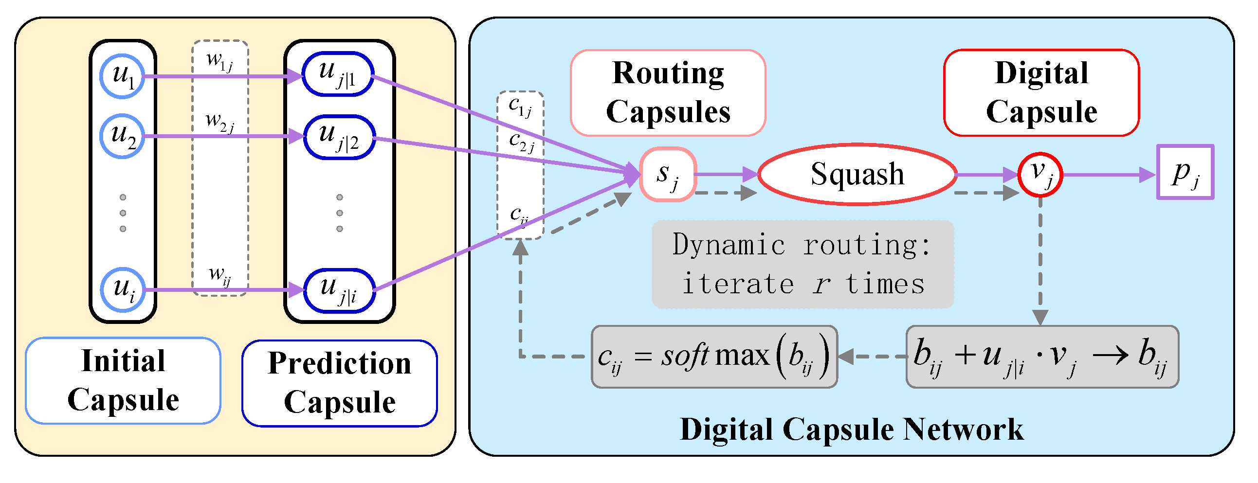
2.2. Capsule Network

The core idea of a capsule network (CN) is to transform each neuron of a traditional neural network from scalar to vector and use a vector as the input and output of the network to reduce the loss of feature information and improve the feature extraction ability of the model. The mode length of the vector represents the probability of a particular health state of the gearbox occurring. The direction of the vector then means the information on the gearbox’s health state. The capsule network mainly consists of an initial capsule layer and a digital capsule layer, and the specific structure is shown in Figure 2.

The process of the capsule network’s operation is as follows:

Step 1: the initial capsule vector $u_i$ is multiplied with the weight matrix $w_{ij}$ to obtain the predicted capsule $u_{j|i}$, which can be expressed as (6):

$$u_{j|i}=w_{ij}{u}_i$$

(6)

Step 2: the prediction capsule $u_{j|i}$ is weighted and summed with the coupling coefficient $c_{ij}$ to obtain the routing capsule $s_j$, where the coupling coefficient $c_{ij}$ is obtained through the intermediate variable $b_{ij}$, using softmax to ensure that all $c_{ij}$ are non-negative and sum to 1, as well as that all initial values of $b_{ij}$ are 0:

$$c_{ij}=soft\max \left(b_{ij}\right)=\frac{\exp \left(b_{ij}\right)}{{\displaystyle {\sum }_{1\le k\le j}\exp \left(b_{ik}\right)}}$$

(7)

$$s_j={\displaystyle \sum _i{c}_{ij}{u}_{j|i}}$$

(8)

Step 3: compress the routing capsule using the Squash activation function, which can preserve the spatial information of the feature vector, i.e., keep the direction of the capsule vector unchanged while compressing the modal length of the capsule to 0~1 to obtain the digital pill $v_j$:

$$v_j=Squash\left(s_j\right)=\frac{{‖s_j‖}^2}{1+{‖s_j‖}^2}\frac{s_j}{‖s_j‖}$$

(9)

Step 4: The digital capsules are optimized by iteratively updating $b_{ij}$ and $c_{ij}$ through a dynamic routing algorithm. The dynamic routing algorithm is an iterative process that continuously adjusts the parameters of the initial capsule layer and the digital capsule layer to improve the gearbox fault diagnosis performance. The initial capsule must decide how to send its output vector to the routing capsule. The initial pill changes the scalar weight, and the output vector is multiplied by that scalar weight and sent to the routing capsule as input to the digital capsule layer. The correlation between the two is first calculated by predicting the inner product of the capsule $u_{j|i}$ and the digital capsule $v_j$. The intermediate variable $b_{ij}$ is optimized by:

$$b_{ij}+u_{j|i}\cdot v_j\to b_{ij}$$

(10)

Then, $c_{ij}$ is updated according to Equation (7). If the correlation between the two capsules is high, the value of their coupling coefficient $c_{ij}$ will increase, and vice versa will decrease. Subsequently, the dynamic routing is iterated through the formula, optimizing $s_j$ and obtaining $v_j$. A total of $r$ iterations were taken in this paper, as $r=3$ [19]. Finally, the optimal numerical capsule $v_j$ is obtained, whose direction indicates a particular health state of the gearbox, and the mode length indicates the probability of the occurrence of this state $p_j$:

$$p_j=‖v_j‖$$

(11)

2.3. Marginal Loss Function

In this paper, the marginal loss (margin loss) is used as the loss function, which can effectively expand the difference between classes and reduce the difference within classes. The calculation formula is as follows:

$$L_c\left(p_c\right)=T_c\max {\left(0,m^{+}-p_c\right)}^2+\lambda \left(1-T_c\right)\max {\left(0,p_c-m^{-}\right)}^2$$

(12)

where $c$ is the fault class; $L_c$ denotes the marginal loss of class $c$ fault; and $p_c$ denotes the probability value of the final output of the model. $T_c$ is the indicator function, $T_c=1$ means the class $c$ fault exists, and $T_c=0$ means the class fault does not exist. $m^{+}$ and $m^{-}$ are the upper and lower bounds, respectively. $m^{+}=0.9$ and $m^{-}=0.1$ in this paper, i.e., the loss value is 0 for $p_c>0.9$, or $p_c<0.1$ when the loss value is 0. $\lambda$ is a scaling factor to adjust the ratio of these two items, and the matter taken here was 0.5.

3. Fault Diagnosis Method Based on Efficient Channel Attention Capsule Network

3.1. Efficient Channel Attention Module

Efficient channel attention (ECA) [28] is a lightweight, plug-and-play attention module with good generalization capability to improve the performance of CNN architectures. The ECA module is processed as shown in Figure 3, given an input feature map $F_{in}$ of size $C\times W$, where $C$ is the number of channels, and $W$ is the width. Figure 3 provides a schematic diagram of the efficient channel attention module.

Step 1: aggregate the spatial information using global average pooling (GAP) to obtain the spatial information description vector $a$:

$$a=GAP\left(F_{in}\right)$$

(13)

Step 2: $a$ is deformed and processed using one-dimensional convolution to achieve local cross-channel information interaction; then, the channel attention weight $M_c$ is obtained by the sigmoid activation function, where the size of the convolution kernel is adaptively selected according to the number of channels in the input feature map, calculated as follows:

$$M_c=Sigmoid\left(conv\left(reshape\left(a\right)\right)\right)$$

(14)

$$k=\psi \left(C\right)={\left|\frac{{\log }_2^{\left(C\right)}}{\gamma }+\frac{b}{\gamma }\right|}_{odd}$$

(15)

where $\gamma$ and $b$ are both constants, and ${\left|t\right|}_{odd}$ indicates that the nearest odd number $t$ is taken.

Step 3: multiply the $M_c$ deformation with $F_{in}$ to obtain the feature map $F_{re}$, corrected by channel attention.

$$F_{re}=F_{in}\ast reshape\left(M_c\right)$$

(16)

3.2. Efficient Channel Attention Capsule Network

The architecture of the efficient channel attention capsule network constructed in this paper is shown in Figure 4, which mainly includes the input layer, convolutional layer, ECA module, initial capsule layer, digital capsule layer, and classification layer. The network processing procedure is as follows:

(1)

The vibration signal sample ${\mathrm{X}}_1,{\mathrm{X}}_2,{\mathrm{X}}_3,\cdot \cdot \cdot ,{\mathrm{X}}_n$ is input from the input layer, and the fault feature $F_{in}$ is finally obtained using one-dimensional convolutional step-by-step feature extraction. It is worth noting that the method uses wide convolutional kernels in convolutional layer 1, which can extract global features and reduce the effect of noise. In addition, the kernel sizes of the subsequent convolutional layers are chosen as narrow convolutional kernels, which become progressively smaller as the network level deepens, fully exploiting the local features.

$$F_{in}=conv4\left(conv3\left(conv2\left(conv1\left(\mathrm{X}\right)\right)\right)\right)$$

(17)

(2)

The ECA module assigns weights to the features of different channels in $F_{in}$ and obtains the attention-corrected feature map $F_{re}$. Channel attention can enhance critical fault information, suppress useless information, and solve the feature redundancy problem.

$$F_{re}=ECA\left(F_{in}\right)$$

(18)

(3)

In the initial capsule layer, five groups of convolution are performed on $F_{re}$, the features of which can be further extracted. After convolution, the scalar values in the feature matrix are spliced to construct 320 initial capsules with a capsule dimension of 5. For the initial capsules, the spatial relationship is represented by each corresponding capsule because of the large number of pills. Since the initial and digital tablets are weighted mapping relationships, the number of digital capsules decreases, but the fault information embedded in each capsule increases. In the digital capsule layer, the dynamic routing algorithm is used to calculate the correlation between the initial capsule and the digital capsule, update the weights, complete the conversion between the pills to realize the accurate categorization of fault information and, finally, generate six digital tablets with a capsule dimension of 10.

(4)

The two-parametric number of the digital capsules is calculated to obtain the probability of the different gearbox health $p$ states, as in Equation (11).

In this paper, compared with the traditional CNN fault diagnosis method, firstly, a GELU was used as the activation function to introduce a nonlinear transformation to the network while adding random regularization, which makes the network converge faster and become more robust. Secondly, an efficient channel attention module was introduced, which can assign weights to different fault information learned by the network, highlighting the fault information that plays a vital role in the diagnosis decision and suppressing useless and harmful information, effectively solving the feature redundancy problem. Finally, the traditional pooling layer was discarded in favor of a capsule network using a dynamic routing algorithm. It thoroughly explores the fault features and maximally preserves their spatial information through vector neurons to obtain better fault diagnosis performance than a traditional CNN.

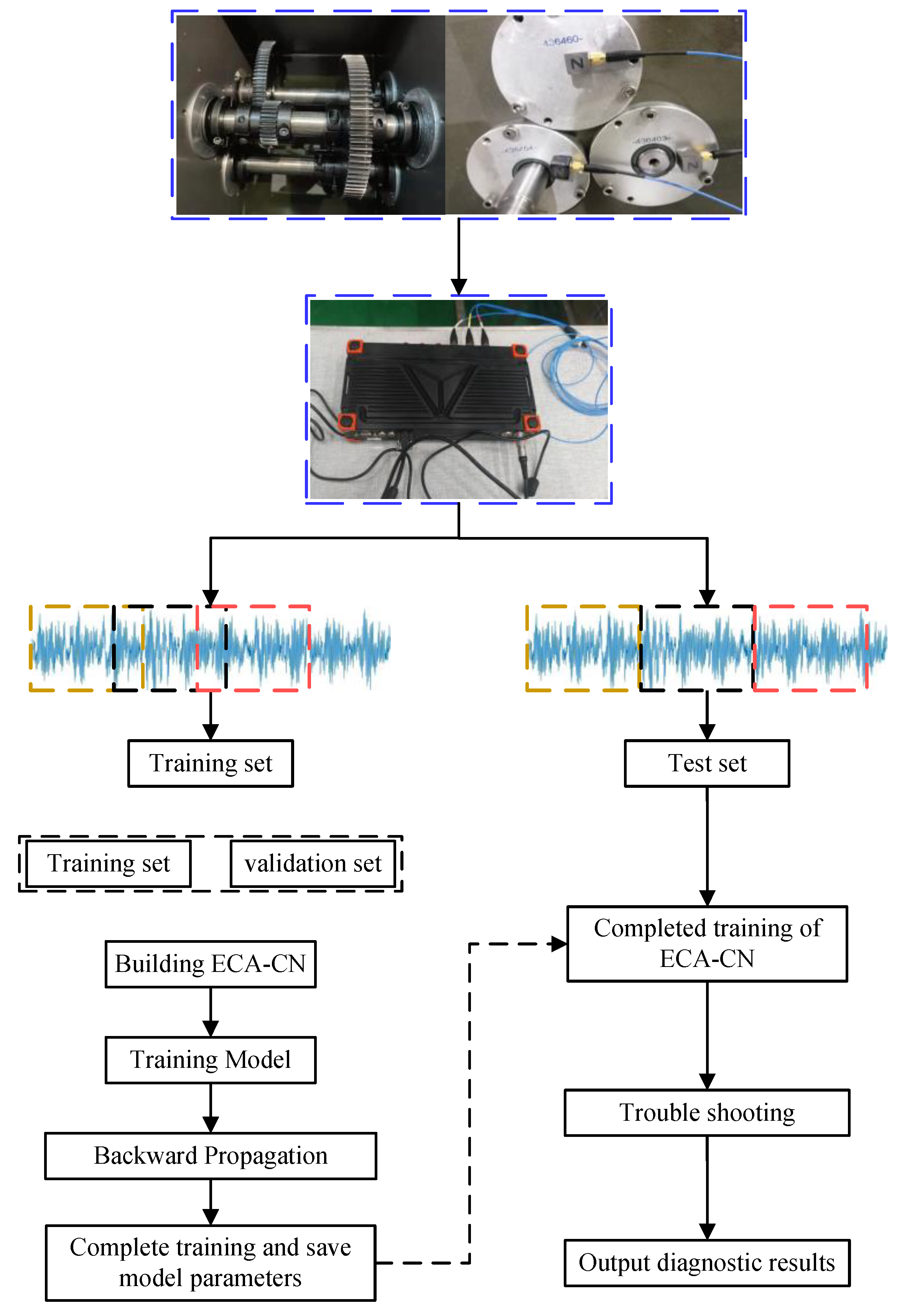
3.3. Fault Diagnosis Process

In this paper, the CNN, ECA, and CN were combined to build a deep learning network that can be used for the compound fault diagnosis of gearboxes under different speed conditions, and its diagnosis process is shown in Figure 5. The specific diagnosis steps are as follows:

(1)

Collect the vibration data of the gearbox at different rotational speeds using acceleration sensors.

(2)

Overlap sampling of the vibration data is performed to obtain the training set. The leave-out method randomly divides the training set into a new training set and a validation set. To prevent information leakage of the test set, the vibration data are routinely window sampled to obtain the test set.

(3)

Construct the ECA-CN model and initialize the parameters.

(4)

Train the model using the training set, select the optimal model based on the validation set, and save the model parameters.

(5)

Evaluate the final model using the test set and derive the diagnosis results.

4. Experimental Verification

4.1. Experimental Data Introduction

To verify the effectiveness and superiority of the method in this paper, the gearbox dataset from the 2009 PHM Challenge [29] was used as the experiment’s fault data. This dataset is divided into two groups: spur gears and helical gears; the helical gear data were selected in this paper. A sketch of the gearbox structure is shown in Figure 6, which contains six bearings and three drive shafts (i.e., input, intermediate, and output shafts), where the gears on the output and input shafts have 16 and 40 teeth, respectively. The number of teeth for the two bags on the intermediate shaft are 48 and 24, respectively.

The vibration data were collected under a low load of the gearbox at 30 Hz, 40 Hz, and 50 Hz, with a sampling frequency of 66.7 kHz and a sampling time of 4 s. A time domain diagram of the collected signals is shown in Figure 7. In this experiment, the sampling window length was 2048, the overlapping sampling moving step was 500, 1500 samples were overlapped for each working condition, and 600 samples were routinely sampled. All models and labels are shown in detail in

Table 1. The description of samples and labels.

Health Status	Sample Length	Overlap Sampling	Conventional Sampling	One-Hot Label Vector
1	2048	1500	600	[1,0,0,0,0,0]
2	2048	1500	600	[0,1,0,0,0,0]
3	2048	1500	600	[0,0,1,0,0,0]
4	2048	1500	600	[0,0,0,1,0,0]
5	2048	1500	600	[0,0,0,0,1,0]
6	2048	1500	600	[0,0,0,0,0,1]
Total	-	9000	3600	-

, and the six health states of the gearbox are described in

Table 2. The description of the gearbox’s health condition.

Serial Number	Health Status	Gear				Bearings						Shaft
		16 T	48 T	24 T	40 T	1	2	3	4	5	6	Input	Output
Case 1	1	N	N	N	N	N	N	N	N	N	N	N	N
Case 2	2	N	N	M	N	N	N	N	N	N	N	N	N
Case 3	3	N	N	B	N	N	C	N	I	N	N	A	N
Case 4	4	N	N	N	N	N	C	N	R	N	N	S	N
Case 5	5	N	N	B	N	N	N	N	I	N	N	N	N
Case 6	6	N	N	N	N	N	N	N	N	N	N	A	N

M: missing tooth; B: broken teeth; C: composite fault; I: inner ring failure; R: rolling element fault; A: axis bending; S: shaft imbalance.

. The samples obtained from the overlap sampling were randomly assigned into a training set and a validation set, where 8000 models were in the training set, 1000 samples in the validation set, and 1000 samples were randomly selected from the samples obtained from the conventional sampling as the test set.

4.2. Ablation Experiments

To verify the effectiveness of the ECA-CN, it was compared with the ECA-CN (ReLU) and a capsule network without ECA, i.e., CN (GELU). The graphics card used in this experiment was an NVIDIA GeForce RTX 3070, the Python version was 3.7, the deep learning framework was Pytorch, and the specific parameters set are shown in

Table 3. The experimental parameter settings.

Parameter Item	Parameter Setting
Loss function	Margin loss
Sample lot Size	64
Training rounds	30
Optimization algorithm	Adam
Learning rate	0.001
Learning rate decay factor	0.0001
Dropout	0.5

. In this paper, we added dropout to the network to avoid overfitting. Dropout can randomly set the weights of some neurons to 0 during the training process of the web so that some neurons can be disabled and the number of parameters can be reduced, thus avoiding overfitting.

Figure 8 shows the three models’ training set loss and accuracy curves. Comparing the ECA-CN with the ECA-CN (ReLU), it can be seen that the loss curve and accuracy curve of the method in this paper converged faster. This is because the GELU avoids the problem of gradient disappearance when the input is negative, and the expressiveness of the model is improved. The GELU also had an adaptive dropout function to enhance the robustness of the model. Compared with the CN (GELU), it is evident that the ECA-CN (GELU) method in this paper, which uses the ECA module, converged faster. The main reason is that the ECA module can assign weights to different channel features, which can focus the attention of the network on the critical fault information and give less weight to other news, thus improving the learning efficiency of the neural network, i.e., speeding up the convergence of the network.

Figure 9 shows the test set confusion matrix of the three models. Cases 1~6 denote the six gearbox health states, the horizontal axis indicates the predicted working condition category, and the vertical axis denotes the actual working condition category. The diagonal, orange areas represent the prediction accuracy of each condition, and the remaining green spaces indicate the misclassification rate. The accuracy of the ECA-CN (GELU) was better than the ECA-CN (ReLU) and the CN (GELU) in all working conditions, and the accuracies of the test set were 99.71%, 99.29%, and 98.51%, respectively, which proves that the method is feasible.

To further illustrate the method’s effectiveness in this paper, the t-distributed stochastic neighbor embedding (t-SNE) algorithm was used to map the feature maps output from each layer of the ECA-CN to a two-dimensional space for feature visualization, as shown in Figure 10. From the plots in Figure 10a–d, it can be seen that the feature extraction of the original vibration signal was performed using one-dimensional layer-by-layer one-dimensional convolution, and the resulting features became increasingly evident as the network layer deepened. This indicates that combining large and small convolution kernels is effective, with the large convolution kernels acquiring a larger sensory field and global mining features. In contrast, the subsequent small convolution kernels were used to further develop local information. As seen from Figure 10e, after four convolution layers, the clusters obtained from clustering each class of samples became apparent. In addition, comparing Figure 10f with Figure 10e, we can see that the output features of the ECA module were more crowded than the clusters clustered by its input features. This is because the ECA module can give weight to the network features, highlighting the fault features critical for diagnostic decisions and suppressing the features that are meaningless for fault classification or even lead to misclassification. Moreover, comparing Figure 10f–h, the plots show that the clusters of fault categories were completely separated after the feature extraction in the capsule layer. This also indicates that the ECA-CN can achieve “end-to-end” fault diagnosis from the original vibration signal to the fault classification. This further validates the effectiveness of the proposed method for compound fault diagnosis in gearboxes with variable speed.

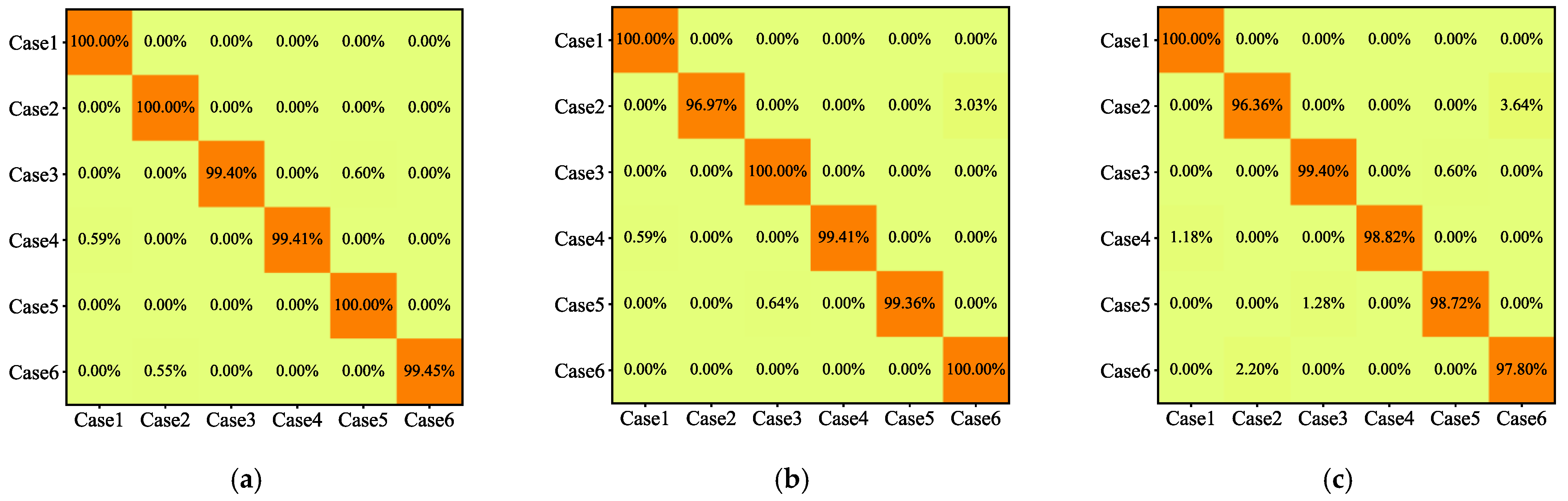
4.3. Comparison Experiments

To verify the superiority of the ECA-CN over convolutional neural networks and shallow machine learning models, it was compared with a CNN [30], fully connected neural network (FNN) [30], support vector machine (SVM) [30], random forest (RF) [30], and wavelet transform-multilabel convolutional neural network (WT-MLCNNN) [31]. To avoid specificity and chance, ten parallel experiments were conducted with the experimental parameters set as shown in Table 3, and the obtained results are shown in

Table 4. The results of 10 parallel experiments of the ECA-CN (%).

Health Status	1	2	3	4	5	6	7	8	9	10	Average Accuracy Rate	Standard Deviation
1	100	100	100	100	100	99.37	100	100	100	100	99.93	0.19
2	99.39	99.39	100	98.18	100	98.79	99.39	100	99.39	100	99.45	0.57
3	99.40	100	100	98.21	100	100	100	100	97.62	100	99.52	0.83
4	100	100	99.41	99.41	99.41	99.41	99.41	100	99.41	99.41	99.58	0.27
5	100	100	99.36	99.36	100	99.36	99.36	100	100	99.36	99.68	0.32
6	100	99.45	98.90	100	99.45	100	100	99.45	99.45	100	99.67	0.36
Test set	99.79	99.80	99.61	99.19	99.81	99.48	99.69	99.90	99.31	99.79	99.63	0.22

.

The comparison results are shown in Figure 11, where the CNN and RF using frequency data as input achieved a 99.33% and 97.24% accuracy, respectively. Similarly, the FNN and SVM using manually extracted frequency features as information gained a 91.62% and 92.83% accuracy, respectively. Although all these shallow models achieve good diagnostic accuracy, they cannot achieve end-to-end fault diagnosis. In contrast, the ECA-CN (GELU) method in this paper used raw vibration data as input, and the average accuracy was 99.63% with a standard deviation of only 0.22%, which indicates that the ECA-CN can effectively extract the composite fault characteristics of gearboxes at different speeds and can accurately achieve end-to-end fault diagnosis. Compared with the WT-MLCNN, which also uses raw vibration data as input, its accuracy was only 94.02% with a standard deviation of 0.75%; the method in this paper shows a more competitive performance.

5. Conclusions

This paper proposed an intelligent diagnosis model with an efficient channel attention capsule network for the compound fault diagnosis of gearboxes at different speeds, which can realize “end-to-end” intellectual fault diagnosis from raw vibration data to fault identification. This method uses a deep convolutional neural network to extract fault features, introduces the ECA module for feature filtering, and uses a capsule network to retain the spatial information of features, which can achieve accurate fault diagnosis. The effectiveness and superiority of the method were verified using the 2009 PHM Challenge gearbox dataset:

(1)

The ECA-CN model uses a GELU as the activation function, and the experimental results show that the ECA-CN (GELU) converges faster and is more robust than the ECA-CN (ReLU);

(2)

The ECA-CN model introduces the ECA module, and the experimental results show that the CN has an accuracy of 99.70%, while the accuracy of the CN without the attention module is 98.68%, indicating that the ECA module can effectively improve the fault diagnosis accuracy of the model;

(3)

Compared with the shallow machine learning model and the traditional CNN model, the average accuracy of the ECA-CN is improved by 4.62%, and the standard deviation is reduced by 0.58%, showing a more competitive fault diagnosis performance, which can achieve the compound fault diagnosis of gearboxes at different rotational speeds.

In future work, we will further develop a decoupling diagnosis for gearbox compound faults based on this paper.

References

1. Qian, Q.; Qin, Y.; Luo, J.; Wang, Y.; Wu, F. Deep discriminative transfer learning network for cross-machine fault diagnosis. Mech. Syst. Signal Process. 2023, 186, 109884. [Google Scholar] [CrossRef]
2. Chen, X.; Guo, Y.; Xu, C.; Shang, H. A review of wind power equipment fault diagnosis and health monitoring research. China Mech. Eng. 2020, 31, 15. [Google Scholar]
3. Zhang, D.; Yu, D.; Zhang, W. Energy operator demodulating of optimal resonance components for the compound faults diagnosis of gearboxes. Meas. Sci. Technol. 2015, 26, 115003. [Google Scholar] [CrossRef]
4. Meng, L.; Su, Y.; Kong, X.; Xu, T.; Lan, X.; Li, Y. Intelligent fault diagnosis of gearbox based on differential continuous wavelet transform-parallel multi-block fusion residual network. Measurement 2023, 206, 112318. [Google Scholar] [CrossRef]
5. Chen, B.; Zhang, W.; Gu, J.X.; Song, D.; Cheng, Y.; Zhou, Z.; Gu, F.; Ball, A.D. Product envelope spectrum optimization-gram: An enhanced envelope analysis for rolling bearing fault diagnosis. Mech. Syst. Signal Process. 2023, 193, 110270. [Google Scholar] [CrossRef]
6. Gu, J.; Peng, Y. An improved complementary ensemble empirical mode decomposition method and its application in rolling bearing fault diagnosis. Digit. Signal Process. 2021, 113, 103050. [Google Scholar] [CrossRef]
7. Xu, B.; Li, H. A Novel Empirical Variational Mode Decomposition for Early Fault Feature Extraction. IEEE Access 2022, 10, 134826–134847. [Google Scholar] [CrossRef]
8. Pi, J.; Liu, P.; Ma, S.; Liang, C.; Meng, L.; Wang, L. Fault diagnosis of aerospace bearings based on MGA-BP network. Vibration. Test Diagn. 2020, 40, 9. [Google Scholar]
9. Cao, H.; Sun, P.; Zhao, L. PCA-SVM method with sliding window for online fault diagnosis of a small pressurized water reactor. Ann. Nucl. Energy 2022, 171, 109036. [Google Scholar] [CrossRef]
10. Wang, H.; Li, S.; Song, L.; Cui, L. A novel convolutional neural network based fault recognition method via image fusion of multi-vibration-signals. Comput. Ind. 2019, 105, 182–190. [Google Scholar] [CrossRef]
11. Qian, Q.; Qin, Y.; Wang, Y.; Liu, F. A new deep transfer learning network based on convolutional auto-encoder for mechanical fault diagnosis. Measurement 2021, 178, 109352. [Google Scholar] [CrossRef]
12. Zhou, J.; Qin, Y.; Luo, J.; Wang, S.; Zhu, T. Dual-thread gated recurrent unit for gear remaining useful life prediction. IEEE Trans. Ind. Inform. 2022, 1–11. [Google Scholar] [CrossRef]
13. Zhou, J.; Qin, Y.; Luo, J.; Zhu, T. Remaining useful life prediction by distribution contact ratio health indicator and consolidated memory GRU. IEEE Trans. Ind. Inform. 2022, 1–11. [Google Scholar] [CrossRef]
14. Xu, Q.; Jiang, H.; Zhang, X.; Li, J.; Chen, L. Multiscale Convolutional Neural Network Based on Channel Space Attention for Gearbox Compound Fault Diagnosis. Sensors 2023, 23, 3827. [Google Scholar] [CrossRef] [PubMed]
15. Yao, D.; Liu, H.; Yang, J.; Li, X.; Cui, X. Research on compound fault diagnosis of urban rail train bearings based on deep learning. J. Railw. 2021, 43, 37–44. [Google Scholar]
16. Zhang, Y.; Zhang, Z.; Shao, F.; Wang, Y.; Zhao, X.; Lv, K. Composite Fault Diagnosis Based on Deep Convolutional Generative Adversarial Network. In Proceedings of the 2020 Asia-Pacific International Symposium on Advanced Reliability and Maintenance Modeling (APARM), Vancouver, BC, Canada, 20–23 August 2020. [Google Scholar]
17. Sun, G.D.; Wang, Y.R.; Sun, C.F.; Jin, Q. Intelligent Detection of a Planetary Gearbox Composite Fault Based on Adaptive Separation and Deep Learning. Sensors 2019, 19, 5222. [Google Scholar] [CrossRef]
18. Yang, Z.B.; Zhang, J.P.; Zhao, Z.B.; Zhai, Z.; Chen, X.F. Interpreting network knowledge with attention mechanism for bearing fault diagnosis. Appl. Soft Comput. 2020, 97, 106829. [Google Scholar] [CrossRef]
19. Woo, S.; Park, J.; Lee, J.Y.; Kweon, I.S. Cbam: Convolutional block attention module. In Proceedings of the European Conference on Computer Vision (ECCV), Munich, Germany, 8–14 September 2018; pp. 3–19. [Google Scholar]
20. Li, X.; Wan, S.; Liu, S.; Zhang, Y.; Hong, J.; Wang, D. Bearing fault diagnosis method based on attention mechanism and multilayer fusion network. ISA Trans. 2021, 128, 550–564. [Google Scholar] [CrossRef]
21. Xie, Y.; Niu, T.; Shao, S.; Zhao, Y.; Cheng, Y. Attention-based Convolutional Neural Networks for Diesel Fuel System Fault Diagnosis. In Proceedings of the 2020 International Conference on Sensing, Measurement & Data Analytics in the Era of Artificial Intelligence (ICSMD), Xi’an, China, 15–17 October 2020. [Google Scholar]
22. Chen, T.; Wang, Z.; Yang, X.; Jiang, K. A deep capsule neural network with stochastic delta rule for bearing fault diagnosis on raw vibration signals. Measurement 2019, 148, 106857. [Google Scholar] [CrossRef]
23. Sabour, S.; Frosst, N.; Hinton, G.E. Dynamic Routing between Capsules. In Proceedings of the Advances in Neural Information Processing Systems 30: Annual Conference on Neural Information Processing Systems 2017, Long Beach, CA, USA, 4–9 December 2017. [Google Scholar]
24. Zhang, Y.; Jiang, Y.; Yang, Y.; Gou, Y.; Zhang, W.; Chen, J. Unknown Compound Faults Diagnosis of High-Speed Train Based on Capsule Network. In Proceedings of the 2019 IEEE 14th International Conference on Intelligent Systems and Knowledge Engineering (ISKE), Dalian, China, 14–16 November 2019. [Google Scholar]
25. Ke, L.; Liu, Y.; Yang, Y. Compound Fault Diagnosis Method of Modular Multilevel Converter Based on Improved Capsule Network. IEEE Access 2022, 10, 41201–41214. [Google Scholar] [CrossRef]
26. Hendricks, D.; Gimpel, K. Gaussian Error Linear Units (GELUs). arXiv 2016, arXiv:1606.08415. [Google Scholar]
27. Cao, X.; Xu, X.; Duan, Y.; Yang, X. Health Status Recognition of Rotating Machinery Based on Deep Residual Shrinkage Network under Time-varying Conditions. IEEE Sens. J. 2022, 22, 18332–18348. [Google Scholar] [CrossRef]
28. Wang, Q.; Wu, B.; Zhu, P.; Li, P.; Zuo, W.; Hu, Q. ECA-Net: Efficient Channel Attention for Deep Convolutional Neural Networks. In Proceedings of the 2020 IEEE/CVF Conference on Computer Vision and Pattern Recognition (CVPR), Seattle, WA, USA, 13–19 June 2020. [Google Scholar]
29. Phm Data Challenge 2009. Available online: https://www.phmsociety.org/competition/PHM/09 (accessed on 10 April 2009).
30. Jing, L.; Zhao, M.; Li, P.; Xu, X. A convolutional neural network based feature learning and fault diagnosis method for the condition monitoring of gearbox. Measurement 2017, 111, 1–10. [Google Scholar] [CrossRef]
31. Liang, P.; Deng, C.; Wu, J.; Yang, Z.; Zhu, J.; Zhang, Z. Compound Fault Diagnosis of Gearboxes via Multi-label Convolutional Neural Network and Wavelet Transform. Comput. Ind. 2019, 113, 103132. [Google Scholar] [CrossRef]
Figure 1. The function image of ReLU and GELU.
Energies 16 04164 g001
Figure 2. The structure of the capsule network.
Energies 16 04164 g002
Figure 3. Schematic diagram of the efficient channel attention module.
Energies 16 04164 g003
Figure 4. Architectural diagram of the efficient channel attention capsule network.
Energies 16 04164 g004
Figure 5. The fault diagnosis process of the ECA-CN.
Energies 16 04164 g005
Figure 6. Structural sketch of the gearbox. 1–6 represents bearings.
Energies 16 04164 g006
Figure 7. Time domain diagram of vibration data.
Energies 16 04164 g007
Figure 8. (a) Loss function curve; (b) accuracy curve.
Energies 16 04164 g008
Figure 9. The confusion matrix of the testing set: (a) ECA-CN (GELU) test set confusion matrix; (b) ECA-CN (ReLU) test set confusion matrix; (c) CN (GELU) test set confusion matrix.
Energies 16 04164 g009
Figure 10. t-SNE visualization of feature maps for each layer of the network: (a) input layer; (b) first convolution layer; (c) second convolution layer; (d) third convolution layer; (e) fourth convolution layer; (f) ECA module; (g) initial capsule layer; (h) digital capsule layer.
Energies 16 04164 g010
Figure 11. Accuracy and standard deviation of each model.
Energies 16 04164 g011