Abstract
The role of interzonal airflows is especially pronounced in naturally ventilated buildings. In such buildings, reversed airflows in the ventilation stacks might occur as well. This affects the air exchange rate and contaminant distribution in buildings. A significant increase in carbon dioxide concentration is a characteristic phenomenon for poorly ventilated rooms. This paper demonstrates the application of metabolic carbon dioxide concentration measurements for interzonal airflow estimation in naturally ventilated buildings. The presented method is based on the continuous measurements of CO2 concentration at one point in each zone. These measurements are used to estimate airflow pattern in a multizone building by applying an inverse analysis. The developed methodology employs an iterative Levenberg-Marquardt procedure to maximise the nonlinear likelihood function. The validity of the method was verified against measurements carried out in a single naturally ventilated room. Further, the method was applied to calculate the airflow pattern in two apartments in Poland, containing 4 and 6 zones. The obtained results revealed very poor ventilation in both investigated apartments and reversed airflow in exhaust ducts. The amount of fresh air entering the rooms was insufficient to ensure good indoor air quality. The developed methodology can be effectively used as a diagnostic tool to identify the potential problems with ventilation systems.
1. Practical Implications
The paper presents a method and program that can be used to estimate the interzonal airflows and their directions in a residential building or apartment. Therefore, it can be used for a ventilation and indoor air quality assessment. The most important advantage of the proposed methodology is that it can be used in an occupied building and it does not disturb the occupants life. The method is based on the information obtained by the continuous measurement of CO2 concentration by a set of sensors. Each room (zone) of the building needs to be equipped with one such sensor. The method is capable to recover airflow patterns in an occupied building. This information can be used to analyse the influence of airflow patterns on contaminants’ distribution and indoor air quality. The significant advantage of the presented method is the ability to predict airflow directions between zones. Moreover, the obtained results can be applied to identify problems and to develop new solutions in natural ventilation, providing a healthier indoor environment.
2. Introduction
Natural ventilation is a dominant type of ventilation system in European households [1]. In Polish dwellings, a passive stack ventilation is the mostly applied natural ventilation system. In this system, air infiltrates to the building interior through the envelope (doors, windows) and is removed by outlets connected to stack ventilation ducts. Due to restricted requirements regarding energy savings and CO2 emission in the last decades, newly-constructed as well as existing buildings have become highly airtight. In many cases, this caused the limitation of the natural air infiltration paths to the building and deterioration of the indoor air quality.
Insufficient ventilation in naturally ventilated buildings results in the increased concentration of indoor air pollutions and poor indoor air quality [2]. Low ventilation influences people’s health and well-being, has an influence on sleep quality and on the next-day performance [1,2,3,4]. Poor ventilation is commonly recognised as one of the reasons of the increased rate of allergy, asthma and other respiratory illness among the inhabitants [3]. Children, in particular, are prone to such illnesses. Moreover, the low quality of indoor air contributes to the productivity loss of workers, affects childrens’ well-being and cause sick-building syndrome (SBS), [5,6,7,8,9,10]. All the arguments suggest that ventilation performance should be monitored at regular intervals to diminish its impact on the health and wellness of inhabitants. Occupancy-based demand-controlled ventilation is the most-used controlling strategy based on CO2 measurements [11,12].
Measurements of the natural ventilation performance in buildings are very difficult due to the unpredictable and stochastic nature of this ventilation type. The exhaustive review of the available methods for the prediction of ventilation rate in the buildings with their strengths and weaknesses has been presented in the literature [7,13,14,15]. The measurement techniques commonly used in the buildings are restricted to determine the airflow rate in one zone, one room or a building as a whole [16,17,18]. In many cases, this suffices to characterise the ventilation performance. However, in poorly ventilated buildings in which infiltration paths of fresh air are limited and reversed flows in stacks may occur in hospitals where knowledge on the possible paths of pathogens spreading is very important, the single zone approach is insufficient. In all these situations, the interzonal airflows must be calculated. Sinden [19] proposed a multizone approach to evaluate the air inflow to a building and its internal redistribution based on the tracer gas measurements. Most of the tracer gase methods require specific measurement conditions given in standards and are preferable in unoccupied buildings. This makes those methods troublesome and expensive when being planned to use in inhabited buildings. The tracer gas that can be safely measured in occupied buildings is carbon dioxide.
Presented in the paper, this method uses metabolic carbon dioxide as a tracer gas for the estimation of interzonal airflows in the building. Carbon dioxide meets most of requirements expected from tracer gas, except uniqueness [16]. CO2 is naturally present in the atmosphere, and its concentration is relatively constant and varies between 350–450 ppm [5], which is considered a drawback in the context of tracer gas measurements. Nevertheless, the presence and variation of CO2 in the atmosphere can be easily accounted for by measuring its concentration during the experiment. Sensors for the measurement of the CO2 concentration are readily available and inexpensive comparing to the traditional tracer gas equipment, which is a significant advantage of this tracer gas. In buildings, the main sources of carbon dioxide are people. The significant increase in the carbon dioxide concentration to 2000 ÷ 5000 ppm is characteristic for poorly ventilated rooms [3,10]. Thus, large indoor concentration levels diminish the influence of the non-zero CO2 concentration in the environment. Moreover, the CO2 concentration is widely used as an indicator of indoor air quality and for demand, because it is proportional to bioeffluents’ concentration emitted by people [12,20,21]. In many country standards, there are recommended values of CO2 concentration in buildings. Commonly, a CO2 concentration equal to 1000 ppm is recommend as an upper threshold value for a comfort criterion of indoor air quality [22,23].
The ASTM standard recommends carbon dioxide as a tracer gas for air exchange calculations in a single zone [20]. Penman and Rashid estimated the airflow rate in a single room by the sequential integration of a CO2 balance equation [24]. The other examples of CO2 applications for single zone modelling can be found in [25,26,27].
Methods for the interzonal airflows estimation are dominated by multi-tracer gas methods, in which the number of tracer gases is equal to the number of zones [28,29,30,31]. An alternative approach is based on the successive injection of the same tracer gas in all zones, keeping a predefined time interval between subsequent injections and monitoring the concentration of this tracer gas in all zones at the same time [32,33]. Calculations of the interzonal airflows in four zones using metabolic CO2 were presented by [34]. Chen and Wen [35] estimated the multizone airflow rates based on the synthetic steady state and transient measurements of the CO2 concentration. The application of metabolic CO2 for multizone airflows’ estimation was also presented by [36]. Although the previous studies demonstrated that it is possible in some cases to calculate interzonal airflows from measurements with only one tracer gas, there is no available inverse procedure dedicated to this specific problem that could successfully calculate the interzonal airflows in various building types containing a different number of zones and estimated airflows.
This paper presents a developed inverse methodology for multizone airflows’ estimation based on metabolic CO2 measurements and its practical application in the developed in-house software MULTIZONE to estimate airflows in naturally ventilated dwellings. The developed method uses a maximum likelihood estimator to identify all unknown airflows. The optimum of the nonlinear likelihood function is found by applying the iterative Levenberg-Marquardt procedure. Interzonal airflows can be calculated from monotonous fragments of recorded CO2 concentration curves, which are measured mainly during the night when occupants sleep (concentration build-up), or when occupants are absent (concentration decay). Firstly, the analysis of the influence of the sensor location within a single zone was carried out. Further, CO2 measurements were carried out in two types of naturally ventilated dwellings, which are representative of the Polish housing sector. The first investigated dwelling was located in small detached house, while the second one was located in a multi-storey residential block. The developed inverse procedure can be successfully used to estimate interzonal airflows in multizone buildings. The presented methodology assumes unidirectional airflows between zones but allows also for the prediction of the airflow direction.
3. Method of Interzonal Airflow Estimations
3.1. Mathematical Model of Carbon Dioxide Propagation within Multizone Building
Interzonal methodology was adopted to describe the carbon dioxide propagation across a building or apartment. In this methodology, a single zone constitutes a room with a closed door. Zones contact each other only by small gaps in doors or windows. In the theoretical case of a dwelling containing N zones, in which all zones have contact with each other, it obtains (N2 + N)/2 unknown airflows in total. However, in real buildings, not all zones are interconnected. The number of interzonal airflows closely depends on the specific zone (rooms) layouts in the building, and, in a real case, is significantly smaller than the above-mentioned number.
The mathematical model of the interzonal airflows is expressed by a set of mass conservation equations of air and carbon dioxide in each distinguished zone. The following assumptions are made at the development stage of the mathematical model:
- Carbon dioxide concentration is uniform within a single zone;
- Carbon dioxide concentration in the surroundings is uniform and constant in time;
- Air is treated as an incompressible fluid;
- Flow is isothermal;
- Unidirectional airflows are assumed between zones.
Usually, assumptions number two, three and four are fulfilled with good accuracy (are easy to meet). The first assumption on the uniformity of carbon dioxide concentration in the presence of occupants and airflows from zones with a different level of carbon dioxide concentration is often not fulfilled [37]. However, [38] demonstrated that it is possible to find a region in the single zone in which the CO2 concentration is a good representation of an average value.
Under the assumptions given above, the mass conservation equations of carbon dioxide for building with N-zones can be simplified to a set of first order ordinary differential equations, which, in a building divided into N zones, are written as follows:
where is the volume of zone i in the N-zone apartment, refers to the carbon dioxide concentration in zone i, stands for the volumetric flow rate from zone j to zone i, N is the number of zones in the apartment, refers to the carbon dioxide emission in zone i and t is time; indexes i = 0, j = 0 identifies the outdoors. This system of the ordinary differential Equation (1) needs to be supplemented with a set of initial conditions in each zone:
where stands for the initial carbon dioxide concentration in zone i. In the inverse procedure described in the next section, this value is taken from the measurements.
Assuming incompressible isothermal flow and ignoring the temporal variations of the airflow due to wind and its turbulence, the set of mass conservation equations for the air in each zone can be written in the following form:
Equation (3) states that the inflow of the air to the zone is equal to the outflow of the air from that zone.
The system of Equation (1) with the initial condition given by (2) and constraints on the airflow rates (3) can be solved to obtain a temporal variation of CO2 concentration in a single zone, if the following quantities are known:
- Volume of each single zone ,
- Carbon dioxide emission rates in each zone ,
- Airflow rates between zones and between zones and outdoors . This assignment is referred to as a forward problem.
In the conducted measurements of CO2 concentration in the indoor air, the only source of the CO2 was the metabolic emission by inhabitants. The emission of carbon dioxide depends on the level of physical activity, body size, diet and sex of the person and can be calculated from equations given in the literature [12,20].
The last set of quantities necessary to solve CO2 conservation in Equation (1) is the matrix of interzonal airflows. The direct measurement of these airflows is very difficult, because it is not possible to identify all the possible leakages in the building and between zones. Hence, any attempt of carrying out such measurements is burdened with high uncertainty. In the next section, the estimation methodology of interzonal air flows based on the measurement of the temporal history of the metabolic CO2 concentration is presented.
3.2. Inverse Problem Formulation
Determination of the interzonal and outdoor airflows in the multizone building based on the measured time history of tracer gas concentration is referred to as an inverse problem. In this work, the unknown air flow rates were estimated by the minimisation of the weighted least square norm:
where is the objective function—the normalised sum of squared deviation between measured and calculated carbon dioxide concentrations, refers to a column vector of the estimated airflows, and stand for the measured and calculated concentrations of carbon dioxide in zone at the time instant , appropriately. Sums in Equation (4) are taken over recording time instants in all zones in the multizone apartment/building. Squared deviations between measured and calculated carbon dioxide concentrations are weighted with variances of the measurement errors . It was assumed to be equal to the squared standard uncertainty for a single sensor. Assuming that the CO2 concentration errors are normally distributed, the minimisation of norm (4) is equivalent to the maximum likelihood estimation of unknown airflow rates [39].
It should be noted that the estimated airflow rates are constrained by a set of conservation equations (3). The number of those conservation equations corresponds to the number of zones in the apartment/building. For multizone systems that have at least two zones, the number of unknown interzonal air flow rates is always higher than the number of constrained conservation equations. Hence, the inverse problem of the airflow estimations described by objective function (4) and constraints (3) can be considered as a non-linear-constrained optimisation problem, for which the decision vector is comprised of the estimated interzonal airflows. The Levenberg-Marquardt method was suitable to solve the presented inverse problem. A Levenberg-Marquardt method is an iterative method for solving the nonlinear optimisation problems [40,41]. This algorithm is particularly useful when the objective function is defined as a weighted or ordinary least square norm. The algorithm can be interpreted as a blend of the steepest descent and Gauss methods. At the beginning of the procedure, when it is far from the problem solution, it carries out the steepest descent iterations, avoiding degeneracy in the Hessian matrix. As the algorithm approaches the problem solution, it tends to the Gauss iterative technique, offering quadratic convergence [41,42].
3.3. Solution Procedure of the Inverse Problem
The analysed inverse problem is formulated as the minimisation of the sum of the squared deviation between the measured CO2 concentrations in distinguished zones and CO2 concentrations calculated using the multizone mathematical model (see Section 2). However, the sought interzonal air flow rates are constrained with air mass balances (3). Therefore, among all interzonal air flow rates written in the vector , two subsets are distinguished. The first subset encompasses the air flow rates estimated by the minimisation of the least square norm (4). The second subset of air flow rates include those that are calculated with a set of equations (3); they are marked as . In zones, the building/apartment in which the interzonal airflows (both between zones and between the zones and surrounding) can be identified, the airflows need to be estimated, while the airflows can be calculated with constraints. For each analysed multizone building/apartment structure, the calculated air flows are chosen in such a way that the set of Equation (3) is non-singular. The described unknown airflows’ distribution is introduced into the objective function (4) and airflow constraints (3), which, written in the matrix form, gives:
where the vector of deviations between measured and calculated concentrations is defined as:
The weighting matrix has an inverse of the variances of carbon dioxide concentration measurements on its main diagonal. Matrices and are the connection matrices describing the connections between the pairs of arbitrary zones and identifying whether the given airflow belongs to the calculated or estimated subset. These matrices are composed of zeros and ones only. One means that connections exist and hence the existing airflows need to be calculated or estimated. Zero means that there are no connections between a given pair of zones.
The constrained non-linear least square problem (5–6) was solved with use of the Levenberg-Marquardt algorithm. The algorithm is slightly modified compared to the original version in order to take the constraining equations into consideration. At each +1 iteration of the algorithm, the estimated airflows are obtained by the solution of the following linear set of equations:
where: is the regularisation parameter and is the identity matrix. is the sensitivity matrix calculated for airflows at iteration k, and in the explicit form can be written as:
The elements of the sensitivity matrix are calculated by approximating the partial differences using the central differences method:
where defines the relative change of the estimated airflow under consideration. The nonlinear parameter estimation problem belongs to the group of ill-conditioned problems. Hence, the aim of the regularisation term is to dampen oscillations and instabilities due to the ill-conditioned character of the matrix approximating the Hessian matrix. The relatively high value of the regularisation parameter is assumed at the beginning of the iterative procedure; further, as the procedure converges, it is gradually reduced. The procedure is stopped when the values of the estimated airflows do not change significantly between two subsequent iterations:
where is the assumed calculation tolerance.
Figure 1 presents the Levenberg-Marquardt solution procedure, which was customised to solve the described inverse problem. In each iteration of the Levenberg-Marquardt procedure, the initial value problem described by a system of equations (1–2) needs to be solved. In this work, it is carried out using the 8th order Dormand-Prince method with an adaptive time step [41], which offers the highest accuracy, among other common methods.
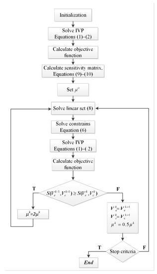
Figure 1.
Solution procedure of the inverse problem.
As the convergent values of the estimated set of airflows are obtained, the covariance matrix for those airflows can be calculated assuming the zero value of the regularisation parameter, as follows:
The covariance matrix allows one to assess the confidence intervals for estimated airflows [39,41,42], as the main diagonal is comprised of the variances of the estimated parameters (estimated airflows). Keeping in mind the linear set of constraints (6), the variances of the set of calculated airflows can be obtained using the propagation of uncertainty rule [43]:
4. Measurements
4.1. Measurements’ Setup
Measurements of the carbon dioxide concentration for the estimation of the interzonal airflows were performed in two dwellings. The first one was located in a residential building on the ground floor, and the second one was situated on the third floor in a multifamily house (Figure 2). The layout of the rooms in each of the dwellings is presented in Figure 3. Both were divided into zones, in such a way that each room with a closed door and window constitutes a separate zone. Dwelling I consisted of four zones and dwelling II consisted of the six zones. In each zone, one sensor was placed. Carbon dioxide sensors were distributed in the most representative location in each zone according to the guidelines provided in the literature [20,38,44].
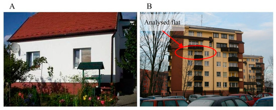
Figure 2.
View of measured buildings; (A)—apartment I (ground floor); (B)—apartment II (third floor).
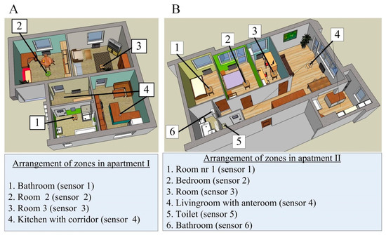
Figure 3.
A plan view showing the arrangement of the zones; (A) – apartment I; (B) – apartment II.
Both buildings have plastic frame windows and are insulated with foamed polystyrene. The operating ventilation system in the buildings is natural ventilation based on the stack effect. The fresh air inflows to the building by leakages in the doors and windows. No additional trickle vents are installed in the windows. In dwelling I, air is usually removed from the rooms through the outflow duct situated in the kitchen. In the dwelling II, air should be removed through the air grating in the toilet and kitchen. The only source of carbon dioxide in both apartments was from people. In dwelling I, two persons were sleeping during the night, one in room 2 and one in room 3. During the day, the number of people varied from 0 to 4. In dwelling II, 3 persons were present during the measurements, 2 adults and one 8-month-old child. During the night, all of them were sleeping in the bedroom 2. The measurements were performed continuously for 6 days in dwelling I and for 20 days in dwelling II.
In both dwellings, indoor air quality (IAQ) parameters were measured, namely: carbon dioxide concentration, temperature and relative air humidity. Additionally, in the dwelling II, the air velocity was measured in the door gap to room 1, to verify the air exchange rate calculated based on the carbon dioxide recordings. The IAQ parameters were recorded continuously with 1 min intervals. The carbon dioxide concentration and temperature in dwelling I were measured using sensors SenseAir® 2001 AT with a measurement range of 0–3000 ppm for the carbon dioxide concentration and −10 +60 °C for temperature. The humidity was measured using the Humitter® 50U/50Y sensor with a measurement range of 0 ÷ 100%. In dwelling II, the measurements were performed using Sensotron® PS33 IAQ monitors, which have built in carbon dioxide, temperature, humidity and barometric pressure sensors. The measured range of CO2 concentration by the IAQ monitor was equal to 0÷5000 with an absolute uncertainty of ±20 ppm + 3% of the measured value.
The velocity of the air in the door gap of room 1 (in apartment II) was measured using DeltaOhm® DO2003 with the thermoanemometer sonde AP471, with a measurement range of 0.4 ÷ 40 m/s and uncertainty of 0.1 ÷ 0.8 m/s. The direction of the air flow was visualised by the smoke generation.
4.2. Measurements’ Results
Carbon dioxide concentration curves recorded in apartment I for two selected days from measurements are shown in Figure 4. A high concentration of CO2 was observed in room and 3 during the night when people were sleeping. With one sleeping person, the concentration in the room increased to 1500 ppm. During the day after people had left the house, the CO2 concentration decreased below 1000 ppm. The measured carbon dioxide concentration in dwelling II is presented in Figure 5. The highest carbon dioxide concentration was observed during the night in the bedroom (where 3 people were sleeping), and it reached 2800 ppm. Most of the time, the carbon dioxide concentration was maintained on the level above 1000 ppm in the entirety of dwelling II. A significant increase in carbon dioxide concentration was observed in the bedrooms in both dwellings when people were sleeping.
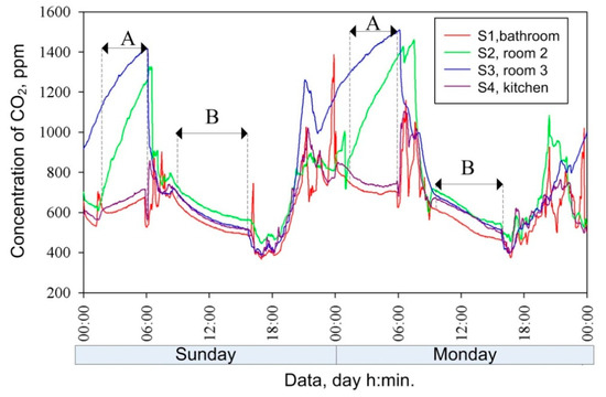
Figure 4.
Measured carbon dioxide concentration in apartment I; A—period of build-up concentration; B—period with decay concentration.

Figure 5.
Measured carbon dioxide concentration in apartment II.
To calculate the interzonal airflows, the monotonic fragments of CO2 concentration curves were selected. Fragments with decreasing CO2 concentration curves occurred when the emission of carbon dioxide was equal to zero, which took place when no occupants were in the building. The monotonic build-up of carbon dioxide concentration arises due to the constant emission of carbon dioxide in time, mainly during night. Fragments with fluctuating CO2 curves were disregarded, as those fluctuations are caused by opening and closing doors and windows separating individual zones. In such conditions, the equations (3) are invalid.
Most commonly, the monotonic behaviour of CO2 curves could be detected during the night hours when occupants were sleeping, and their metabolic activity was almost constant. That is why these periods are the best for interzonal airflow estimations based on CO2 measurements. Knowing the numbers of occupants in each zone, the emission of carbon dioxide concentration was calculated. Figure 4 presents the selected periods with a build-up (A) and decay (B) of CO2 concentration. The zones’ volumes were known; the initial CO2 concentrations were assumed based on the measurements.
5. Results
5.1. Results: Model Validation
The empirical validation of the developed inverse methodology was performed for one zone model. It was conducted by comparing the estimated air change rate from carbon dioxide concentration measurements with the air change rate calculated based on the measurements of air velocity in the door gap of the analysed room. These measurements were performed in the room number 1 in the second dwelling (see Figure 3).
For these validation measurements, four sensors were distributed in the room. The first sensor (sensor 1) was placed in the centre of the room, 1.8 m above the floor. The second one (sensor 2) was positioned just in the corner of the room 0.2 m from its walls and the floor. The third sensor (sensor 3) was placed in the centre of the room on its floor. The forth sensor (sensor 4) was located near the metabolic source of CO2 [38]. The air change rate for the analysed room was calculated with inverse methodology based on the measurements in all four points as well as based on the average CO2 concentration in the room. Table 1 presents the results of the estimated air change rate based on CO2 concentration measurements in the room with values calculated from the velocity measurement in the door gap. The results are presented for a consecutive three days of measurements. Differences between inverse estimation and direct velocity measurement for all analysed cases were within the uncertainty of velocity measurements.

Table 1.
Comparison of calculated air change rate from velocity measurement with air change rate estimated from CO2.
Other factors that influence the calculated air change rate, except sensor position, are the errors in the measurement of carbon dioxide concentration. Therefore, the influence of the systematic and random error of the measured CO2 on the calculated air change rate was analysed.
The systematic measurement was simulated by the shifting of the original CO2 concentration curve by a constant bias. The measurement burden with a random error was generated by adding the normally distributed noise with a standard deviation equal to the assumed value. The three ranges for carbon dioxide concentration errors, as in [40], were considered:
- Tolerance level I—±10% average value of carbon dioxide concentration in the room. This tolerance interval is permitted by the standard [12,13] for carbon dioxide concentration oscillation within one zone during the measurements;
- Tolerance level II—± accuracy of carbon dioxide sensors. Accuracy of the sensors in the measurements was equal to 20 ppm ±3% of the measured value;
- Tolerance level III—±20 ppm, minimal estimated value of the measurement uncertainty.
Analysis of the systematic error showed significant influence on the estimated air-flows (Table 2). For tolerance level I, the values of the estimated flows have changed by approximately 26% comparing to the original values. Approximately for tolerance level II, the flow values have changed by 12% and for tolerance level III by 4%. The influence of random errors on the estimated air change rate is much smaller than it was observed for the systematic errors. For the measurement tolerance level I, an average air flow error was in the order of 9%, for tolerance level II it was 7% and for tolerance level III it was appropriately 3%—Table 3.
Table 2.
Analysis of systematic errors of measured CO2 concentration on estimated air change rate.
Table 3.
Analysis of the random errors of measured CO2 concentration on estimated air change rate.
5.2. Results: Estimation of Airflows in Occupied Dwellings
The mathematical models of the CO2 propagation based on the interzonal approach presented in Section 2 was built for both apartments. Further, the monotonic periods of the time history of carbon dioxide concentration in each zone of both apartments were selected for the inverse estimation of interzonal air flows. The arrangement of the zones in each apartment is presented in Figure 6.

Figure 6.
Model of interzonal air flow rate; (A) – apartment I; (B) – apartment II.
One-directional flows were assumed for estimation purposes. This assumption is realistic for the situation when airflows can occur in small gaps in the doors only. Moreover, it was assumed that the air inflows to the rooms from outside (surrounding) and is removed from the apartments through the exhaust duct (in zone 4 in dwelling I and in zone 4, 5 and 6 in dwelling II). Figure 6 also presents the assumed direction of the interzonal flows. The inverse procedure permits the negative values of the estimated airflows, which denote that the direction of the airflows in the zone is opposite to the assumed one.
5.3. 4-Zones; Apartment I
Calculations in apartment I were run for the 16 selected monotonic fragments of the CO2 concentration curves. Fragments with a build-up of carbon dioxide concentration occurred in the occupied zones. The emission of CO2 calculated for people sleeping in zone 2 was assumed to be constant and equal to 0.010 m3/h in zone 2 and equal to 0.0099 m3/h in zone 3. In the case of CO2 concentration decay, it took place during a day when no occupants were present in the apartment and the emission of carbon dioxide was equal to zero. Table 4 shows the results of the calculated interzonal airflows in apartment I together with the estimation uncertainties. In bedrooms 2 and 3, the air inflows from outside and outflows to zone 4. The values of the airflow rates in bedrooms 2 and 3 were very small and did not exceed 0.13 h−1 for zone 2 and 0.15 h−1 for zone 3 with one incidental value of 0.5 h−1 in zone 3. In zone 1 (bathroom), the estimated airflow rate was of the order of 2 ÷ 5 m3/h (0.01 ÷ 0.23 h−1) when the window was closed. For a case with a window slightly opened in the bathroom (which took place during the night on the 2nd of April and 3rd of April), the airflows had an opposite direction, which means that the airflow went from zone 4 to zone 1 and was then removed outside. The opposite direction of the airflow to the assumed one is denoted with a negative sign of the airflow value in Table 4. Zone 4 in apartment I is a cumulative zone to which all airflows flow in from neighbouring zones. The air from zone 4 is then removed through the outflow duct located in that zone or partially through zone 1. For all interzonal airflows calculated with inverse analysis, te good fitting between measured and estimated CO2 curves was obtained, as it is presented in Figure 7. The value of the objective function described by Equation (7) did not exceed 4.75∙10−4 for all analysed cases.
Table 4.
Results of the estimated airflows in apartment I for selected monotonic fragments of CO2 concentration curves.

Figure 7.
Fitting of the estimated and calculated curves of carbon dioxide concentration in apartment I for cases from.
5.4. 6-zones in Apartment II
The inverse calculations in apartment II were run for 11 selected monotonic fragments of CO2 concentration curves. The constant build-up of carbon dioxide concentration was recorded in the night when occupants were sleeping in zone 2. At the same time, in the remaining zones, the concentration of CO2 was slowly decreasing. The emission of CO2 calculated for 3 people present in zone 2 (2 adults and one child) was assumed to be constant when sleeping and equal to 0.029 m3/h. A few fragments of decreasing carbon dioxide concentration curves (in all zones) during a day with no emission of CO2 were also selected.
Table 5 shows the values of estimated airflows rates with uncertainties calculated for the selected days of measurements. The only two cases gave some reasonable results. The rest of the analysed cases with very small differences of CO2 concentration between individual rooms failed due unacceptable uncertainty intervals. The fresh air inflows to apartment II through zones 1 ÷ 4 from the surroundings and then should be removed outside through the air ducts in zone 4, 5 and 6; see Figure 6. Hoverer, in one of the analysed cases (case 2), the reversed flow in zones 5 and 6 was found. The same situation was observed in zone 4 in the other case. The inhabitants confirmed that this situation occurs frequently during the heating season. The amount of the inflowing air in zone 5 and 6 was very small and usually did not exceed 1 m3/h for the analysed cases.
Table 5.
Results of the estimated airflows in apartment II for selected monotonic fragments of CO2 concentration curves.
The calculated airflow rates in zones 1 to 3 demonstrated insufficient ventilation of those rooms. The corresponding number of the air change rate did not exceed 0.3 h−1 in zone 1, 0.8 h−1 in zone 2 and 0.4 h−1 in zone 3. In those rooms, the direction of the calculated air flows agreed with the assumed ones. The amount of the fresh air flowing through the bedroom was not able to provide a proper indoor air quality for three sleeping persons. The fitting of the estimated and calculated curves of the carbon dioxide concentration in apartment II for the selected cases is presented in Figure 8.
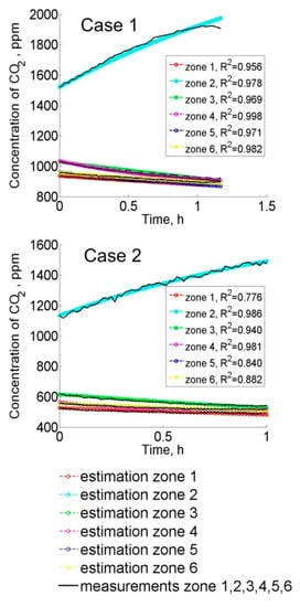
Figure 8.
Fitting of the estimated and calculated curves of carbon dioxide concentration in apartment II for cases presented in Table 5.
6. Discussion
The accurate estimate of the airflows in the building is very important for evaluating indoor air quality in buildings, as well as the ventilation performance and energy use. Ventilation performance in buildings influences peoples’ health and well-being. Available in literature models for interzonal airflow calculations estimate the bidirectional airflows using the multi-tracer gas procedure [24,27] or introducing one tracer gas to n − 1 zones in the building and repeating the procedure one at a time [28]. It was demonstrated that the developed method is available to identify the amount and directions of the airflows, assuming one directional airflow between the zones. The method requires solving the inverse problem based on the known time history of carbon dioxide concentration in each zone. This information has a significant meaning to track the air and contaminants’ flow pattern in the building. The presented method is easy, non-invasive, provides a quick estimate of the airflows’ rates in the buildings and is much cheaper compared to the other tracer gas methods used for the estimation of interzonal airflows. The main advantage of this method is that it can be used in occupied buildings using CO2, exhaled by people, which reduces the costs of tracer gas purchases. The novelty of the method presented in this paper relays the purposely developed inverse procedure that works well with carbon dioxide concentration data, extending the findings of [20,30]. In the first step, the theoretical verification of the inverse methodology based on simulated input data was performed. The verification was performed for 2, 3, 4 and 6 zone models for the simulated measurements data obtained with analytical solutions of carbon dioxide balance equations. A very good agreement between the assumed and calculated airflows was observed for all analysed cases (regardless of the number of zones and estimated airflows).
The developed inverse procedure was validated against the measurement data gathered in a single room. The estimated airflows were compared with the value received from the velocity measurements in the door gap. The discrepancy between the estimated and measured airflow was contained within the limits of the uncertainty of the air exchange rate calculated from the velocity measured by the anemometer.
Finally, the developed methodology was applied to estimate the interzonal airflows in real buildings. The calculations were based on the measurement data available for two apartments. The calculation in real buildings demonstrated that the described methodology can be a promising tool for interzonal airflow calculations. Calculated airflow rates in bedrooms for both apartments indicated insufficient ventilation and poor indoor air quality. This problem was particularly intensified during the night, when the door to the bedrooms were closed. The poor ventilation resulted in a very fast increase in carbon dioxide concentration in the rooms. In both apartments, it was assumed that the air flowed into the bedrooms from the surroundings and further spread to neighbouring zones, exiting the apartment through the exhaust duct. The estimated airflows demonstrated that their directions were not always consistent with the assumed ones. In apartment II, only one exhaust duct worked properly, and in the remaining ducts, the airflows were the opposite.
The air exchange rate in zones 1 to 3 in apartment I were also calculated using one zone model as a reference. In that case, it was assumed that the fresh air from the surroundings flows into a zone and then flows out into neighbouring zones, which is a typical assumption made for a one-zone model. Airflows calculated in the one-zone model were compared against values estimated with use of the inverse analysis. A good agreement was obtained for most of the analysed cases, with the exception of the airflows in zone one (apartment I) with a negative value. In that case, the one-zone model fails to find an exact result. However, for a situation with an opposite airflow direction, any comparison of both approaches is meaningless, because the inflowing air has an unknown concentration of CO2, which varies with time; hence, the single zone model cannot be applied. This also confirms the necessity of the multizone model application. The interzonal airflows calculated in apartment II were also compared with the air exchange rate calculated using the single zone model. This was possible for the zones to which the air was inflowing from the outside, namely zones: 1, 2 and 3, but also for zones 5 and 6, only in the case of reversal flows. A very good agreement of the calculated air exchange rates between both models was obtained for both of the analysed cases.
The application of the presented method in a real building may increase the popularity of the ventilation measurements in buildings. Moreover, in the future, it can find an application in the automatic controlling of ventilated windows, trickle ventilators or highly occupied offices. The presented calculation method can be used with other tracer gases, e.g., N2O, which can also be used in occupied buildings. The application of N2O will allow one to eliminate the uncertainty connected with the calculations of carbon dioxide emission from people.
7. Conclusions
As presented in this paper, this method allows one to calculate the interzonal airflows in residential buildings using metabolic carbon dioxide measurements. The method will improve the ventilation measurements’ popularity in residential buildings, which is necessary to improve the indoor air quality and ventilation performance in buildings. The main findings can be summarised:
- The developed inverse procedure works well with a measured one -racer gas concentration in each zone, such as with metabolic carbon dioxide;
- The presented method is easy, non-invasive and provides a quick estimate of the airflow rates in the building;
- Airflows can be estimated during peoples’ presence in the building and after they they leave;
- Long-term measurements can be performed;
- Airflow directions can be estimated.
Author Contributions
Conceptualization, A.B. and Z.B.; Methodology, Z.B.; Software, Z.B.; Formal analysis, Z.B.; Investigation, A.B.; Data curation, A.B.; Writing—original draft, A.B.; Writing—review & editing, Z.B.; Visualization, A.B.; Project administration, A.B. All authors have read and agreed to the published version of the manuscript.
Funding
This research and the APC was funded by the Silesian University of Technology through the grant for statutory research and grant number the Rector’s grant number 08/060/RGJ22/1061.
Data Availability Statement
The data presented in this study are available on request from the corresponding author.
Acknowledgments
The work of Anna Bulinska was supported by the Silesian University of Technology through the grant for statutory research. The work of Zbigniew Bulinski was supported by the Silesian University of Technology through the Rector’s grant number 08/060/RGJ22/1061.
Conflicts of Interest
The authors declare no conflict of interest.
References
- Dimitroulopoulou, C. Ventilation in European Dwellings: A Review. Build. Environ. 2012, 47, 109–125. [Google Scholar] [CrossRef]
- Sundell, J.; Levin, H.; Nazaroff, W.W.; Cain, W.S.; Fisk, W.J.; Grimsrud, D.T.; Gyntelberg, F.; Li, Y.; Persily, A.K.; Pickering, A.C.; et al. Ventilation Rates and Health: Multidisciplinary Review of the Scientific Literature. Indoor Air 2011, 21, 191–204. [Google Scholar] [CrossRef]
- Bekö, G.; Lund, T.; Nors, F.; Toftum, J.; Clausen, G. Ventilation Rates in the Bedrooms of 500 Danish Children. Build. Environ. 2010, 45, 2289–2295. [Google Scholar] [CrossRef]
- Strøm-Tejsen, P.; Zukowska, D.; Wargocki, P.; Wyon, D.P. The Effects of Bedroom Air Quality on Sleep and Next-Day Performance. Indoor Air 2016, 26, 679–686. [Google Scholar] [CrossRef]
- Seppanen, O.; Fisk, W. Summary of Human Responses to Ventilation. Indoor Air Suppl. 2004, 14, 102–118. [Google Scholar] [CrossRef]
- Crook, B.; Burton, N.C. Indoor Moulds, Sick Building Syndrome and Building Related Illness. Fungal Biol. Rev. 2010, 24, 106–113. [Google Scholar] [CrossRef]
- Nazaroff, W.W. Residential Air-Change Rates: A Critical Review. Indoor Air 2021, 31, 282–313. [Google Scholar] [CrossRef]
- Bogdanovica, S.; Zemitis, J. The Effect of CO2 Concentration on Children’s Well-Being during the Process of Learning. Energies 2020, 13, 6099. [Google Scholar] [CrossRef]
- Moultanovsky, A.V. Mobile HVAC System Evaporator Optimization and Cooling Capacity Estimation by Means of Inverse Problem Solution. Inverse Probl. Eng. 2002, 10, 1–18. [Google Scholar] [CrossRef]
- Ma, F.; Zhan, C.; Xu, X. Investigation and Evaluation Ofwinter Indoor Air Quality of Primary Schools in Severe Cold Weather Areas of China. Energies 2019, 12, 1602. [Google Scholar] [CrossRef]
- Wang, W.; Shan, X.; Hussain, S.A.; Wang, C.; Ji, Y. Comparison of Multi-Control Strategies for the Control of Indoor Air Temperature and Co2 with Openmodelica Modeling. Energies 2020, 13, 4425. [Google Scholar] [CrossRef]
- Emmerich, S.J.; Persily, A.K. State-of-the-Art Review of CO2 Demand Controlled Ventilation Technology and Application. NIST In Interagency/Internal Report (NISTIR), National Institute of Standards and Technology, Gaithersburg, MD. 2001. Available online: https://tsapps.nist.gov/publication/get_pdf.cfm?pub_id=860846 (accessed on 25 November 2022).
- Allard, F. Natural Ventilation in Buildings: A Design Handbook; James & James Science Publishers: London, UK, 1998. [Google Scholar]
- Etheridge, D. Natural Ventilation of Buildings: Theory, Measurement and Design. In Natural Ventilation of Buildings: Theory, Measurement and Design; Wiley: Hoboken, NJ, USA, 2011. [Google Scholar] [CrossRef]
- Persily, A.K. Field Measurement of Ventilation Rates. Indoor Air 2016, 26, 97–111. [Google Scholar] [CrossRef]
- Sherman, M.H. Tracer-Gas Technique for Measurements Ventilation in a Single Zone. Build. Environ. 1990, 25, 365–374. [Google Scholar] [CrossRef]
- ASTM. E 741–00; Standard Test Method for Determining Air Change in a Single Zone by Means of a Tracer Gas Dilution. American Society for Testing and Materials: West Conshohocken, PA, USA, 2000.
- ISO 12569:2017; Thermal Performance of Buildings and Materials—Determination of Specific Airflow Rate in Buildings—Tracer Gas Dilution Method. ISO: Geneva, Switzerland, 2017.
- Sinden, F. The Multi-Chamber Theory of Air-Infiltration. Build Environ. 1978, 13, 21–28. [Google Scholar] [CrossRef]
- ASTM. Standard D 6245-18; Standard Guide for Using Indoor Carbon Dioxide Concentration to Evaluate Indoor Air Quality and Ventilation. American Society for Testing and Materials: West Conshohocken, PA, USA, 2002.
- Angelova, R.A.; Markov, D.; Velichkova, R.; Stankov, P.; Simova, I. Exhaled Carbon Dioxide as a Physiological Source of Deterioration of Indoor Air Quality in Non-Industrial Environments: Influence of Air Temperature. Energies 2021, 14, 8127. [Google Scholar] [CrossRef]
- CEN. CR 1752; Ventilation for Buildings—Design Criteria for the Indoor Environment. European Committee for Standardization: Brussels, Belgium, 1998.
- Hedrick, R.L.; Thomann, W.R.; Aguilar, H.; Damiano, L.A.; Darwich, A.K.H.; Gress, G.; Habibi, H.; Howard, E.P.; Petrillo-groh, L.G.; Smith, J.K.; et al. Ventilation for Acceptable Indoor Air Quality. ASHRAE Stand. 2010, 8400, 1–70. [Google Scholar]
- Penman, J.M.; Rashid, A.A.M. Experimental Determination of Air-Flow in a Naturally Ventilated Room Using Metabolic Carbon Dioxide. Build. Environ. 1982, 17, 253–256. [Google Scholar] [CrossRef]
- Lu, T.; Knuutila, A.; Viljanen, M.; Lu, X. A Novel Methodology for Estimating Space Air Change Rates and Occupant CO2 Generation Rates from Measurements in Mechanically-Ventilated Buildings. Build. Environ. 2010, 45, 1161–1172. [Google Scholar] [CrossRef]
- Roulet, C.; Foradini, F. Measurement of Infiltration Rates from the Daily Cycle of Ambient CO2. International Journal of Ventilation. Int. J. Vent. 2016, 14, 409–420. [Google Scholar]
- Cui, S.; Cohen, M.; Stabat, P.; Marchio, D. CO2 Tracer Gas Concentration Decay Method for Measuring Air Change Rate. Build. Environ. 2015, 84, 162–169. [Google Scholar] [CrossRef]
- Sherman, M.H. On the Estimation of Multizone Ventilation Rates from Tracer Gas Measurements. Build. Environ. 1989, 24, 355–362. [Google Scholar] [CrossRef]
- Sherman, M.H. Uncertainty in Air Flow Calculations Using Tracer Gas Measurements. Build. Environ. 1989, 24, 347–354. [Google Scholar] [CrossRef][Green Version]
- Miller, S.L. Nonlinear Least-Squares Minimization Applied to Tracer Gas Decay for Determining Airflow Rates in a Two-Zone Building. Indoor Air 1997, 7, 64–75. [Google Scholar] [CrossRef]
- Sohn, M.D.; Small, M.J. Parameter Estimation of Unknown Air Exchange Rates and Effective Mixing Volumes from Tracer Gas Measurements for Complex Multi-Zone Indoor Air Models. Build. Environ. 1998, 34, 293–303. [Google Scholar] [CrossRef]
- Afonso, C.F.A.; Maldonado, E.A.B.; Skåret, E. A Single Tracer-Gas Method to Characterize Multi-Room Air Exchanges. Energy Build. 1986, 9, 273–280. [Google Scholar] [CrossRef]
- Oneill, P.; Crawford, R. Identification of Flow and Volume in Multizone Systems Using a Single-Gas Tracer Technique. Ashrae Trans. 1991, 49–54. Available online: https://ui.adsabs.harvard.edu/abs/1991STIN...9119368O/abstract (accessed on 25 November 2022).
- Smith, P.N. Determination of Ventilation Rates in Occupied Buildings from Metabolic CO2 Concentrations and Production Rates. Build. Environ. 1988, 23, 95–102. [Google Scholar] [CrossRef]
- Ng, L.C.; Wen, J. Estimating Building Airflow Using CO2 Measurements from a Distributed Sensor Network. HVAC R Res. 2011, 17, 344–365. [Google Scholar] [CrossRef]
- Bulinska, A. Determination of Airflow Pattern in a Residential Building Using Metabolic Carbon Dioxide Concentration Measurements. In Proceedings of the 10th International Conference on Air Distribution in Rooms, SCANVAC Conference, Roomvent, Helsinki, Finland, 13–15 June 2007. [Google Scholar]
- Mahyuddin, N.; Awbi, H. The Spatial Distribution of Carbon Dioxide in an Environmental Test Chamber. Build. Environ. 2010, 45, 1993–2001. [Google Scholar] [CrossRef]
- Bulińska, A.; Popiołek, Z.; Buliński, Z. Experimentally Validated CFD Analysis on Sampling Region Determination of Average Indoor Carbon Dioxide Concentration in Occupied Space. Build. Environ. 2014, 72, 319–331. [Google Scholar] [CrossRef]
- Beck, J.; Arnold, K. Parameter Estimation in Engineering and Science; John Wiley & Sons Inc.: Hoboken, NJ, USA, 1977. [Google Scholar]
- Ozisik, M.; Orlande, H.R. Inverse Heat Transfer. Fundamentals and Applications; Tylor and Francis: Abingdon, UK, 2000. [Google Scholar]
- Press, W.; Flannery, B.; Teukolsky, S.; Wetterling, W.T. The Art of Scientific Computing, 3rd ed.; Cambridge University Press: Cambridge, UK, 2007. [Google Scholar]
- Dantas, L.B.; Orlande, H.R.B.; Cotta, R.M. An Inverse Problem of Parameter Estimation for Heat and Mass Transfer in Capillary Porous Media. Int. J. Heat Mass Transf. 2003, 46, 1587–1598. [Google Scholar] [CrossRef]
- Johnson, R.; Wichern, D. Applied Multivariate Statistical Analysis, 6th ed.; Pearson Education, Inc.: New York, NY, USA, 2007. [Google Scholar]
- Mahyuddin, N.; Awbi, H.B. A Review of CO2 Measurement Procedures in Ventilation Research. Int. J. Vent. 2012, 10, 353–370. [Google Scholar] [CrossRef]
Disclaimer/Publisher’s Note: The statements, opinions and data contained in all publications are solely those of the individual author(s) and contributor(s) and not of MDPI and/or the editor(s). MDPI and/or the editor(s) disclaim responsibility for any injury to people or property resulting from any ideas, methods, instructions or products referred to in the content. |
© 2022 by the authors. Licensee MDPI, Basel, Switzerland. This article is an open access article distributed under the terms and conditions of the Creative Commons Attribution (CC BY) license (https://creativecommons.org/licenses/by/4.0/).