Multi-Criterial Assessment of Electric Vehicle Integration into the Commercial Sector—A Case Study

Abstract

Transforming the transport sector to zero emission is an integral part of changes to the energy sector worldwide. This effects not only the electrification of the private sector but also the commercial sector. The aim of this study is to develop methodologies, algorithms and associated requirements for the integration of electric vehicles into a logistics application with a possible reduction in operating costs. The most favorable solution for a company was evaluated using the analytic hierarchy process algorithm considering three main aspects: economic, environmental and technical. An analysis of the environmental impact of the vehicle fleet in terms of atmospheric emissions was also conducted, based on the data available for combustion and electric vehicles, considering the well-to-tank approach. The costs associated with operating an electric vehicle were identified and compared to the current costs associated with operating a standard diesel-based fleet. Incorporating the identified costs of electrifying the vehicle fleet, an algorithm was implemented to reduce the number of vehicles in the company and, thereby, significantly reducing the costs associated with fleet maintenance.

1. Introduction

New regulations concerning the introduction of new ecological energy sources to the market are in line with the European Union (EU) policy, the Green Deal, on combating climate change. Consequently, the automotive industry is also seeking and placing emphasis on the development of electromobility (e-mobility) and the associated charging infrastructure. The new regulations proposal, setting the target of at least 55% net emission reduction by 2030 [1], forces European countries to reduce emissions in the transport sector, which is responsible for 21.76% of CO₂ pollution in relation to other economic sectors worldwide [2]. This means that increased the production and development of electric vehicles (EVs) is inevitable, and European cities will enjoy less air pollution and improved living comfort.

The increase in the number of vehicles brings many benefits to society, as described in Noel et al. [3,4], most notably reducing CO₂ [5] and particulate matter (PM10) emissions [6] and lowering exploitation costs, but it will also create new challenges for the transmission and distribution system operator [7,8]. The increase in electricity demand is an integral part of the transformation of the transport sector. Furthermore, vehicles, whose charging process has been described by various authors [9,10,11,12], have a significant impact on momentary changes in the power distribution in the system. The issue is well-known and has been described quite extensively [13,14]. Simulation results were published by Chen et al. [15] which indicate an increase in the energy demand by 3% in the local power grid after the installation of 60 charging stations for electric buses. Other articles indicate a projected increase in energy consumption within the distribution network [16].

Accordingly, reasonable solutions are being considered to eliminate the messy side effects of vehicle charging [17]. Mechanisms that are currently being developed in the energy market are system services, such as peak load shaving, load management and line loss reduction. These services and implementations have been the subject of research for many years, and a description and example application of a peak shaving service for system needs has been described previously [15,18,19,20]. An example of the application of this service in Shanghai—China being a rapidly developing e-mobility country—has been given by Li et. al. [21]. Other articles [22,23] also describe the possibility of intelligent load management using the regulation capabilities of EVs. Chung et al. [24] also applied modern methods of data analysis based on machine learning, allowing for optimal energy management based on algorithms that predict the behaviour of EV users. The occurrence of power losses, which are an undesirable phenomenon and one that could be eliminated by using the energy resources of EVs, has also been described [25,26]. Moreover, additional system functions for fleets of EVs are also indicated, and have been described in reference materials: spinning reserve [27,28], stabilizing grid voltage [29,30] and frequency control [31,32,33,34].

Rapid changes in EU legislation enforcing reductions of all kinds of emissions and increasing energy consumption in both the industrial and private sectors are driving the energy transition [35,36,37]. A transformation has started with the development of renewable energy sources, the introduction of energy-efficient appliances [38,39,40], and the storage of heat and electricity. In this context, we are increasingly talking about the coupling of energy sectors allowing for greater flexibility in energy supply, load and storage. The principle of this energy sector coupling has been described in detail [41,42] and critically [43]. Development results in the implementation of new technologies, such as 5G-V2X [44,45,46] and machine learning [47] for e-mobility. In the case of the latter, this transformation is taking place at the fastest rate due, among other aspects, to the falling prices of batteries for EVs. Battery prices have fallen by 89%, from a global average of 1200$ US per kWh in 2010 to 132$ US per kWh in 2021 [48]. This has started a trend toward EV fleets dedicated to public transport. Berlin, Germany, for example, ordered 122 e-buses in 2020. Hamburg ordered 583 e-buses, which will be delivered by 2025. Paris, France, has ordered 4500 new e-buses, which will also be delivered by 2025 [48]. In addition, battery-as-a-service technology has been strongly developed in recent years [49,50,51]. The leading manufacturer is NIO from China, which has set up 700 battery replacement facilities since 2000. A report [48] states that this action reduces the price of a vehicle by 10,000$ US.

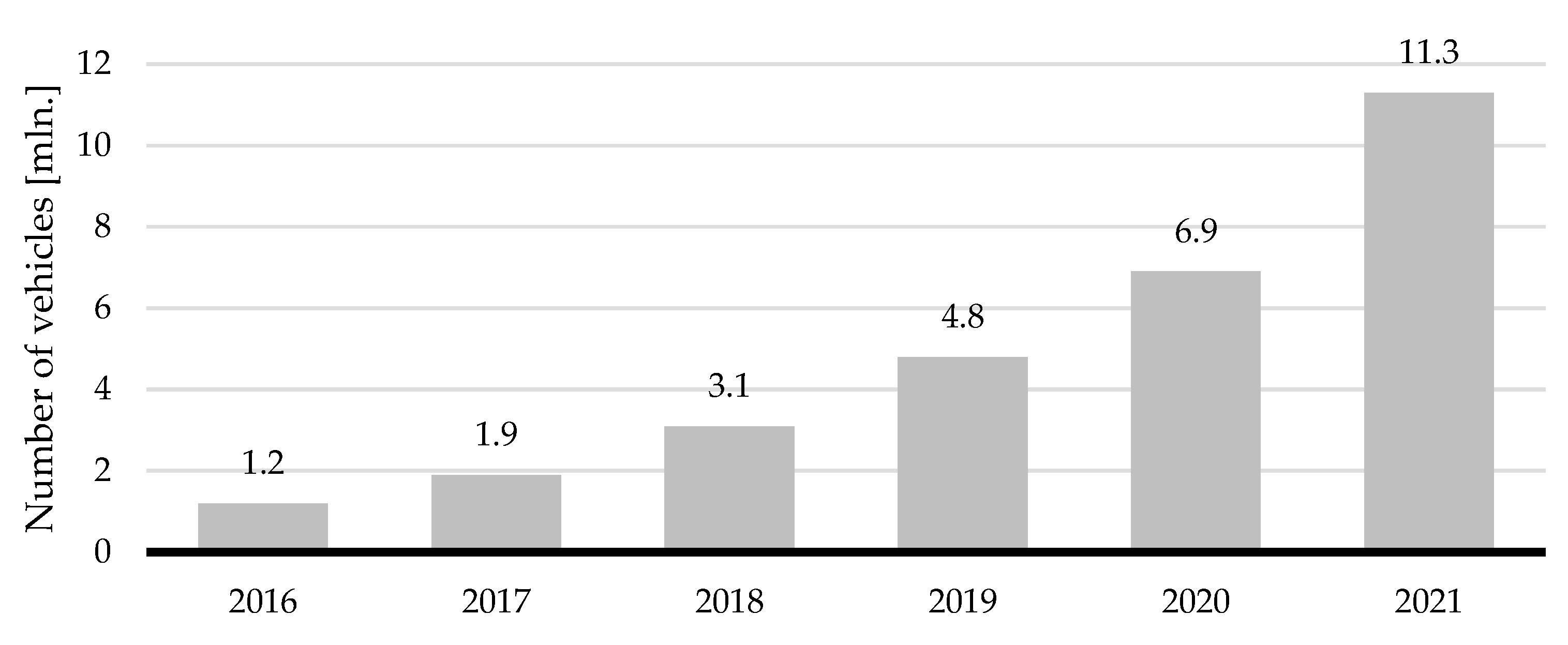
Transport and especially the developing infrastructure of EVs is gaining importance during the energy transition and the merging of energy sectors. Based on the 2021 IEA report [52], it can be observed that there are already more than 10 million vehicles with electric propulsion systems in circulation worldwide, of which 1.5 million are in the EU.

There is also a sharp increase in the number of new EVs due to the tightening of climate policy. Figure 1 shows the change in the number of vehicles worldwide over the past six years.

The development of e-mobility is strictly dependent on the level of CO₂ emissions into the atmosphere, and two possible development scenarios have been adopted by the EU: the Stated Policies Scenario and the Sustainable Development Scenario [52]. Each of them defines the percentage growth of vehicles and charging points until 2030. This growth is related to the replacement of traditional vehicles used by individual users or vehicle fleets of companies and enterprises. There were 14,033 electric, light commercial vehicles in Germany in 2021, making it the second highest in Europe in terms of the use of EVs in the commercial sector [48]. A higher exploitation of the vehicles’ potential occurs in the United Kingdom, Korea and China. This growth is associated with the need to expand the existing charging infrastructure, which is integral to the transformation of this sector. This entails a number of changes, including the need to upgrade supply lines, replace medium- and low-voltage transformers, and expand substations and distribution systems. These changes will be most visible in the networks of companies with significant vehicle fleets, which will be transformed into electric fleets in the near future. This process will mainly affect the load on the network and the costs associated with vehicle modernization. The changes on the part of the distribution network operator and the need to modernize its networks are not relevant for companies. However, the changes resulting from the need to convert the fleet into EVs involves certain investments that the company has to consider and budget for. This process is often time-consuming.

According to one source [54], the number of light commercial vehicles registered in Germany is increasing steadily. Globally, 26.29 million light-duty vehicles (LDVs) and 56.4 million passenger vehicles were sold in 2021 [55]. Commercial vehicles account for about 30% of vehicles sold. The most common use of commercial vehicles is in the supply chain, as shown in Figure 2. The product produced by the manufacturer is initially transported to the sorting facility/warehouse, where it is then transported to the warehouse covering the area for the distribution of goods to the customer. We can now see the electrification of vehicles at stage 3. Companies such as Amazon and DHL Post are already using EVs within cities to deliver ordered products. Stage 1 and 2 electrification is less common and poses a lot more challenges, but it is also feasible. The electrification of the transport sector is the subject of an analysis described previously [56].

The multi-criteria evaluation indicates the benefits of the planned and undertaken measures. In this case, the assessment helps to confirm the benefits of the concurrent development of renewable energy sources as the primary power source for electric vehicles. While electric vehicles are currently popular in the private sector, their further development in other parts of the economy is also advisable. In most scientific works, a multi-criteria assessment is made in relation to the power grid [58,59,60] and the impact of vehicles on the grid, its parameters and system operations. In this case, the work is focused on analyzing the benefits of operating two different types of vehicles for the company, rather than the power grid. The work is intended to encourage companies to change their company model to one that is more beneficial to the environment with minimal investment. The price ratio of raw materials and electricity plays a large role in the decision-making process and also forces not only electric vehicle manufacturers but also internal combustion vehicle manufacturers to take measures to improve efficiency and effectiveness and to reduce the harmful emissions of conventional vehicles, which improves the competitiveness of the automotive market.

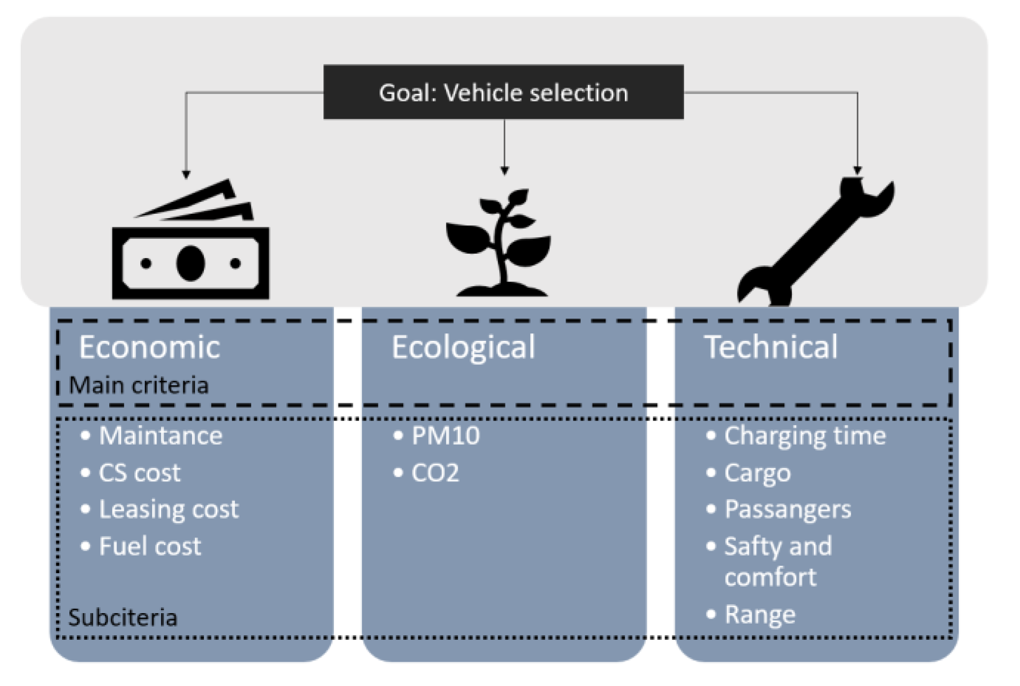
Therefore, this paper presents a model to compare the costs associated with the use of a fleet of combustion vehicles and a corresponding fleet of EVs. The cost associated with the use of vehicles of both types was determined. Based on the analytic hierarchy process (AHP) algorithm, the potential best solution for the company was determined based on three categories (economic, technical and ecological). The AHP method has been used, among other methods, for the dimensioning of microgrid components and has been described previously [61,62]. This description includes analyses based on real statistical and measurement data obtained as part of a realized research project. The economic situation influences the choice of the optimal vehicle significantly. The objective of this study is to examine the impact of changes in electricity and fuel prices on the purchase of a vehicle. In addition, a minimization analysis of the vehicle fleet and the number of charging stations for EVs was carried out based on global positioning system (GPS) measurement data. The aim is to present an algorithm to support the decision-making process that will accompany all enterprises during the transformation of the energy sector.

Section 2 describes the methods used including a description of the AHP algorithm employed, the GPS measurement data used and background information on the vehicle fleet adopted. The limitations and assumptions for the simulation carried out are also listed. Section 3 presents the results of the analyses and simulations carried out. A comparison of the costs associated with the use of two types of vehicles is presented in Section 4, and the costs that companies have to incur when replacing their vehicle fleet are determined. Conclusions are presented in Section 5 based on the analyses carried out and the cost-effectiveness limit is indicated.

2. Materials and Methods

2.1. Multi-Criterial Decision Algorithm

In order to select the variant that meets the requirements best, here the choice of vehicle for the logistics company, it is possible to use known solutions and algorithms supporting multi-criteria decision support, such as the simple additive weighting method (SAW) [63], simple multi-attribute ranking technique (SMART) [64], AHP [65], ratio estimation in magnitudes or decibells to rate alternatives which are non-dominated (REMBRANDT) [66], analytic network process (ANP) [67], elimination et choix traduisant la realia (ELECTRE) [68] and preference ranking organisation method for enrichment evaluations (PROMETHEE) [69,70]. Of the methods best suited to the issue, the AHP method was selected and used due to its simple implementation, optimal result-meeting requirements and simplicity of result interpretation. The AHP, developed by Thomas L. Saaty in the 1970s, is a technique for organizing and analyzing complex decisions. This process is the most accurate approach to quantifying the weights of the criteria that are required to estimate the relative importance of factors (weights) by using appropriate comparisons. It is particularly applicable in group decision-making, where the relative importance between two issues is compared using an appropriately chosen scale. Three stages can be distinguished in the decision-making process:

• The formulation of alternatives;
• The evaluation of alternatives according to one or more criteria; and
• The making of a choice, i.e., selecting one of the alternatives based on the results of the previous evaluations.

This method is based on a series of pairwise comparisons between criteria and gives them a score of relative importance. A percentage weight is calculated for each criterion; the sum of all percentage weights is 100%. “A” is the comparison matrix, a_ij the numerical value resulting from the comparison of criteria “i” and “j” and “n” is the number of criteria. The result of (n(n − 1))/2) comparisons generates the matrix A_nxn which is used to create a vector of percentage weights (or priorities) for each criterion. The subscript “i” represents the rows of the pairwise comparison matrix, while the subscript “j” denotes the columns. It is generally a rating scale that ranges from 1 to 9, where each degree corresponds to the following rating, presented in the

Table 1. Scale for pairwise comparison [65].

The Fundamental Scale for Pairwise Comparisons
Intensity of Importance	Definition	Explanation
1	Equal importance	Two elements contribute equally to the objective
3	Moderate importance	Experience and judgment slightly favor one element over another
5	Strong importance	Experience and judgment strongly favor one element over another
7	Very strong importance	One element is favored very strongly over another; its dominance is demonstrated in practice
9	Extreme importance	The evidence favoring one element over another is of highest possible order of affirmation

.

The $a_{ij}$ values of matrix A has the following properties:

• if $a_{ij}=x$, then $a_{ji}=\frac{1}{x}$ for x > 0;
• if $a_i$ is judged to be of equal intensity relative to $a_j,$ then $a_{ij}=a_{ji}=1.$

In particular, the main diagonal of the matrix A is composed entirely of unit values, i.e., a_ii = 1.

2.1.1. Normalization

After obtaining the matrix A of the pairwise comparisons, the maximum eigenvalue λ and the relative eigenvector $v_{\lambda }$ of the A matrix are determined to calculate the vector of the percentage weights [28]. Normalizing the vector $v_{\lambda }$, the sum of its elements is equal to 1, we obtain the vector of the percentage weights “W” or the priorities:

$$W=\frac{v_{\lambda }}{{{\displaystyle \sum }}_{i=1}^n{v}_{\lambda }\left(i\right)}$$

(1)

2.1.2. Consistency Calculation

Once the priority vector has been determined, it is necessary to understand whether the matrix of pair comparisons is consistent or not, i.e., to measure whether the subjective judgments of the evaluator at each comparison are consistent. The purpose is to make sure that the preference ratings are consistent. First, it is necessary to calculate λ:

$$\lambda ={\displaystyle \sum }_{i=1}^n\frac{{\left(A·v_{\lambda }\right)}_i}{n·v_{\lambda i}}$$

(2)

the consistency index (CI) can then be formulated as follows:

$$\mathit{CI}=\frac{\lambda -n}{n-1}$$

(3)

after that, the consistency ratio (CR) [71] is calculated:

$$\mathit{CR}=\frac{\mathit{CI}}{\mathit{RI}}$$

(4)

Matrix A is classified as a constraint if CR < 0.10 (10%) in the least-restrictive scenario. If the consistency ratio is vast, then the evaluation is not consistent enough, and the best thing to do is to go back and revise the comparisons. This check concludes the first step in the procedure. Based on standardized weights, a score is assigned for each subcriterion while taking into account the hierarchy of criteria. The item with the highest score is the one that meets the user’s needs best.

2.2. Technical Analysis

The comparative analyses use the technical parameters of two vehicles: an internal combustion engine vehicle (ICEV) and a battery EV (BEV) available on the market. Based on these, indicators will be defined to allow a total cost of ownership (TCO), ecological, technical and economic analysis. The vehicle’s performance, characteristics and driving profile, and the infrastructure of the charging stations should be specified accordingly. Measurement data in the form of GPS data from vehicles belonging to a transport company that used an 81 kW, 110 hp, 5-speed manual Nissan NV200 VAN in its fleet were used in this study. They are the input data for further analyses.

2.2.1. Characteristics of the Vehicles

This work bases the various analyses on the comparison between a conventional diesel ICEV vehicle and a BEV. The idea is to compare two models that are similar in size and function (e.g., the provision of transport services). An electric e-NV200 model analogous in design and function was selected for the model for which GPS data were recorded, which differs only in the propulsion system used. The basic parameters of both vehicles are shown in

Table 2. Characteristics of vehicles.

	Nissan NV200 VAN Diesel	Nissan e-NV200 VAN BEV
Vehicle Type	Light-duty commercial	Light-duty commercial
Vehicle Kerb Weight [kg]	1286	1498
Payload [kg]	714	742
Seats	2	2
Propulsion	Diesel ICEV Euro 6	Electric
Acquisition year	2019	2019
Battery capacity, bc [kWh]	-	40
Charging power AC [kW]	-	6.6
Charging power DC [kW]	-	50
Tank capacity, tc [L]	55	-

. Both are LDVs with similar overall weights. The higher weight of the EV is due to the additional heaviness of the battery.

2.2.2. Performance of the Vehicles

Real consumption for both vehicles depends on several factors: driving speed and road characteristics (urban, extra-urban, highway), nature of the route (uphill, downhill, level), outdoor temperature and use of air conditioning, and driving style (ecological, constant, sport). The actual fuel consumption of the Nissan NV200 diesel was assessed based on the GPS data under the assumption that the vehicle was normally used for product transport. Fuel levels were recorded before and after each trip (

Table 3. Performance of vehicles.

	Nissan NV200 VAN Diesel	Nissan e-NV200 VAN BEV
Consumption (Standard)	4.90 L/100 km (NEDC)	25.9 kWh/100 km (WLTP)
Real consumption, rc	8.9 L/100 km	28.1 kWh/100 km
Range	617 km	138 km

NEDC: new European driving cycle; WLTP: worldwide harmonised light vehicles test procedure.

).

The real consumption of the Nissan e-NV200 has been evaluated using experimental test results conducted by the ADAC (allgemeine Deutsche Automobil-Club e. V.). It has not been possible to acquire actual recorded data, since the customer company has not yet had the BEV tested. Actual consumption, as with ICEV, is higher than that stated by the manufacturer. The maximum vehicle range has been determined for the new data according to the formula:

(a)

Nissan NV200 VAN, 81 kW, 110 cv, 5-speed manual, diesel

$$\mathrm{Range}=\frac{\mathrm{tank} \mathrm{capacity} }{\mathrm{real} \mathrm{consumption}}·100$$

(5)

(b)

Nissan e-NV200 VAN:

$$\mathrm{Range}=\frac{\mathrm{battery} \mathrm{capacity}}{\mathrm{real} \mathrm{consumption}}·100$$

(6)

2.2.3. Driving Profile

Tests such as the new European driving cycle (NEDC) or worldwide harmonised light vehicles test procedure (WLTP) [72] are carried out on new vehicles, helping to simulate a realistic car trip even under laboratory conditions. Regarding the scenario applied here, driving profiles were adopted, created on the basis of measurements and then used in the calculations. The registration of measurements was carried out based on the routes of 60 light vehicles belonging to the company’s fleet during one week. The journeys made by the vehicles made it possible to determine the basic parameters (departure time, time in depot, distance traveled, energy consumption). An example of such a route recorded for a vehicle in the course of providing transport services to the company is presented in Figure 3.

2.2.4. Infrastructure of the Charging Stations

When deciding on a fleet of EVs, the company bears the cost of designing and building the charging infrastructure. In the case of vehicles with internal combustion engines, there is no need to address this aspect, as the fuel infrastructure is not the responsibility of the company but is managed by external companies; this incurs additional investment costs. The charging location is the company’s depot, where there are as many parking spaces as there are charging vehicles. The standard Nissan e-NV200 comes with two charging cables: a 10 A Mode charging cable for charging at home using a standard 230 V socket, and a 32 A Mode charging cable for charging at charging stations or wall-boxes.

Table 4. Common charging methods and charging times for EVs [4].

	Number of Phases	Voltage/Current	Power	Plug System	Charging Time for 300 km Range
Slow Charging	1 AC	230 V/10 A	2.3 kW	Schuko	30 h
(<10 kW)	1 AC	230 V/16 A	3.7 kW	Blue CEE socket	19 h
	1 AC	230 V/32 A	7.4 kW	IEC Typ 2	10 h
Accelerated Charging	3 AC	400 V/16 A	11 kW	IEC Typ 2	6.5 h
(11, 22 kW)	3 AC	400 V/32 A	22 kW	IEC Typ 2	3 h
Fast charging	DC	400 V/125 A	50 kW	IEC Typ 2 CCS	90 min
(>50 kW)	DC	400 V/500 A	200 kW		30 min
	DC	800 V/500 A	350 kW		10 min

identifies the most common solutions for charging stations.

2.3. Total Cost Ownership Analysis

The TCO is the sum of the investment and lifetime costs of a vehicle. A distinction is made between the fixed costs associated with the vehicle, infrastructure costs (where applicable) and variable costs. The mathematical procedure for calculating the TCO for both propulsion technologies, Equations (7)–(15), is shown below.

The TCO is expressed in year i:

$${\mathit{TCO}}_i\left({\mathit{rc}; M}_a\right){=C}_{\mathit{FIXi}}{ + C}_{\mathit{VARi}}{ + C}_{\mathit{Li}}{ + C}_{\mathit{FUELi}}{ + C}_{\mathit{CSi}}$$

(7)

where:$\mathit{rc}$—real consumption [L/100km] or [kWh/100km], $M_a$—annual mileage [km/a], $C_{\mathit{FIXi}}$—fixed costs [€/year], $C_{\mathit{VARi}}$—variable costs [€/year], $C_{\mathit{Li}}$—purchase price [€/year], $C_{\mathit{FUELi}}$—fuel costs [€/year] and $C_{\mathit{CSi}}$—infrastructure cost [€/a].

Fixed costs:

$$C_{\mathit{FIXi}}{ = C}_{\mathit{tax}}{ + C}_I{ + C}_S$$

(8)

variable costs:

$$C_{\mathit{VARi}}{ = C}_{\mathit{MAINT}1i}{ + C}_{MAINT2}{ + C}_{TIRESi}$$

(9)

where

$$C_{\mathit{TIRES}i} = \frac{4·C_{\mathit{TIRE} } + C_{\mathit{LAB}}}{M_{\mathit{MAX}}}·M_{\mathit{ai}}$$

(10)

purchase cost:

$$C_{Li} = 12·L$$

(11)

fuel cost:

$$C_{\mathit{FUEL}i} = \frac{{ \mathit{rc}}_i}{100}·P·M_{\mathit{ai}}$$

(12)

infrastructure cost:

$$C_{\mathit{cs}i } = I + m$$

(13)

where

$$I = \{\begin{array}{c} I_{TOT}, \mathrm{Total} \mathrm{investment} \mathrm{payed} \mathrm{in} i = 1\\ I_i, \mathrm{Total} \mathrm{investment} \mathrm{payed} \mathrm{in} i = 5\end{array}$$

(14)

The total investment is calculated over 5 years, i $\in$ [1;5]:

$${\mathit{TCO}}_{\mathit{TOT}}\left({\mathit{rc}; M}_a\right)={\displaystyle \sum }_i{(C}_{\mathit{FIXi}}{ + C}_{\mathit{VARi}}{ + C}_{\mathit{Li}}{ + C}_{\mathit{FUELi}}{ + C}_{\mathit{CSi}})$$

(15)

where:$C_{\mathit{tax}}$—vehicle tax [€/a], $C_I$—insurance cost [€/a], $C_S$—services and inspection costs [€/a], $C_{\mathit{VAR}}$—variable costs [€/a], $C_{\mathit{MAINT}1}$—maintenance and repair costs [€/a], $C_{\mathit{MAINT}2}$—replacement and other maintenance costs [€/a], $C_{\mathit{TIRES}}$—tires replacement costs [€/a], $C_{\mathit{TIRE}}$—one tire price [€], $C_{\mathit{LAB}}$—labor cost [€], $M_{\mathit{MAX}}$—maximum mileage for a tire change [km], $C_{\mathit{FUEL}}$—fuel costs [€/a], P—diesel fuel or electricity price [€/L] or [€/kWh], $C_L$—purchase price [€/a], L—leasing instalment [€/month], $C_{\mathit{CS}}$—infrastructure cost [€/a], I_TOT—total charging station investment [€], $I$—charging station instalment [€] and $m$—infrastructure maintenance [€/a].

2.4. Ecological Analysis

The aim of this section is to assess the magnitude of greenhouse gas (GHG) and PM10 emissions associated with EVs and their changes depending on the structure of electricity generation in Germany, as well as the differences between GHG emissions from BEVs and ICEVs by applying well-to-wheel (WTW) analysis. The most significant potential GHG reductions between BEVs and ICEVs occur during the use phase, which can compensate for the greater impact of the feedstock extraction and production phase (lithium mining for batteries). The BEVs charged with coal-fired electricity currently have higher WTW emissions than ICEVs, while the WTW emissions of BEVs could be almost 90% lower than an equivalent ICEV using electricity generated from renewable sources.

This analysis is structured in four sections:

• Electricity mix: German electricity mix emissions as an example for this case study;
• Oil emissions: emissions from oil production;
• WTW analysis: comparison of CO₂ equivalent and PM10 emissions for the two vehicles compared in the study case; and
• Tire wear emissions: PM10 emissions evaluation.

The EVs are now considered to be the most innovative technology in the transport sector, but their actual effect on the environment is directly related to the electricity generation mix of a country. Therefore, some countries that do not have an environmentally friendly (in terms of GHG emissions) electricity generation mix show that EVs may not be beneficial in reducing GHG emissions [73]. It is necessary to consider the country’s energy mix where the study is conducted, because each energy mix influences the indirect emissions (Figure 4), considered in the WTT and well-to-power plant (WTPP) indices.

2.4.1. Well-to-Wheel Analysis ICEV WTW

The WTW analysis was born as an index of energy efficiency, but it is also used for environmental analysis. The term “well-to-wheel” refers to the entire process of energy flow, from the mining of the energy source to the drive. The following are required in order to determine the WTW emissions:

• the real emissions, in terms of [g⋅CO₂eq/L] and [g⋅CO₂eq/kWh], for the two propulsion systems;
• for calculating BEV indirect emissions:

  ○

  Germany electricity generation mix data [74];

  ○

  GHG emission data of each power source in the WTPP process; and

• for calculating ICEV indirect emissions

  ○

  GHG emission data of diesel fuel in the WTW process.

The GHG emissions of ICEVs, from a WTW perspective, are the sum between the WTT and TTW processes GHG emissions. The PM10 emissions [gPM10/km] are calculated using the same approach.

$${\mathit{WTW}}_{\mathit{ICE}} = \left({\mathit{WTT}}_{\mathit{ICE}}+{\mathit{TTW}}_{\mathit{ICE}}\right)·\frac{\mathit{rc}}{100}$$

(16)

(a)

Wheel-to-Tank

$$\begin{gathered} {\mathit{WTT}}_{\mathit{ICE} {\mathit{CO}}_2}{ = P}_{{\mathit{CO}}_2}·\frac{\mathit{rc}}{100} \\ {\mathit{IE}}_{\mathit{ICE} {\mathit{CO}}_2} = {\mathit{WTT}}_{\mathit{ICE}}·M_a \\ {\mathit{IE}}_{\mathit{ICE} \mathit{PM}10} = P_{\mathit{PM}10}·\frac{\mathit{rc}}{100}·M_a \end{gathered}$$

(17)

where: ${\mathit{WTW}}_{\mathit{ICE}}$—total GHG emissions (WTW approach) [gCO₂eq/km], ${\mathit{WTT}}_{\mathit{ICE}}$—Well-to-Tank GHG emissions [gCO₂eq/L], ${\mathit{TTW}}_{\mathit{ICE}}$—Tank-to-Wheel GHG emissions [gCO₂eq/L], rc—real consumption [L/100 km], $M_a$—annual mileage [km/a], $P_{{\mathit{CO}}_2}$—CO₂ equivalent diesel production [gCO₂eq/L], ${\mathit{IE}}_{{\mathit{ICE} \mathit{CO}}_2}$—indirect CO₂ equivalent emissions [tonCO₂eq/a], $P_{\mathit{PM}10}$—PM10 diesel production [gPM10/L] and ${\mathit{IE}}_{\mathit{ICE}\mathit{PM}10}$—indirect PM10 emissions [gPM10/a].

(b)

Tank-to-Wheel

Direct tailpipe emissions for ICEVs are calculated using CO₂ equivalent tailpipe emissions [kgCO₂eq/a] and PM10 tailpipe emissions [gPM10/a].

$$\begin{gathered} {\mathit{TTW}}_{\mathit{ICE} {\mathit{CO}}_2} = E_{{\mathit{CO}}_2}·\mathit{DS} + E_{\mathit{NOx}}·{\mathit{GWP}}_{\mathit{NOx}} \\ {\mathit{DE}}_{\mathit{ICE} {\mathit{CO}}_2}={\mathit{TTW}}_{\mathit{ICE}}·M_a \\ D{E}_{ICE PM10}=E_{PM10}·DS·M_a \end{gathered}$$

(18)

where: $E_{{\mathit{CO}}_2}$—direct CO₂ tailpipe emissions [gCO₂/km], $DS$—driving style, $E_{\mathit{NOx}}$—direct NOx tailpipe emissions [gNOx/km],${\mathit{GWP}}_{\mathit{NOx}}$—Global Warming Potential Index [75], ${\mathit{TTW}}_{{\mathit{ICE} \mathit{CO}}_2}$—direct CO₂ equivalent tailpipe emissions [gCO₂eq/km], ${\mathit{DE}}_{{\mathit{ICE} \mathit{CO}}_2}$—direct CO₂ equivalent tailpipe emissions [tonCO₂eq/a], $E_{\mathit{PM}10}$—direct PM10 tailpipe emissions [gPM10/km] and ${\mathit{DE}}_{\mathit{ICE} \mathit{PM}10}$—direct PM10 tailpipe emissions [gPM10/a].

2.4.2. Well-to-Wheel Analysis BEV WTW

The BEV WTW process consists of the sum of two contributions:

• WTPP due to the process of mining energy source and transporting it to the power plant; and
• Power plant-to-wheel due to the process of transmitting the electricity to the vehicle and driving it using that electricity.

While electric propulsion in the vehicle is efficient, the overall energy use and GHG emissions depend greatly on the source used to produce electricity. The WTW missions for BEVs are calculated as the sum of each emission by source:

$$WT{W}_{BEV}=\left\{{\displaystyle \sum }_e{R}_e·\left(WTP{P}_{BEVe}+PPT{W}_{BEVe}\right)\right\}·\frac{rc}{100}$$

(19)

where: ${\mathit{WTW}}_{\mathit{BEV}}$—total GHG emissions (WTW approach) [gCO₂eq/km], R_e—ratio of the power source in the German electricity generation mix, ${\mathit{WTPP}}_{\mathit{BEVe}}$—Well-to-Power Plant GHG emissions by the energy source “e” [gCO₂eq/kWh] and ${\mathit{PPTW}}_{\mathit{BEVe}}$—Power Plant-to-Wheel GHG emissions by the energy source [gCO₂eq/ kWh].

(a)

WTPP emissions

$$\begin{gathered} {\mathit{WTPP}}_{{\mathit{BEVCO}}_2} = {\displaystyle \sum }_e\left({\mathit{GHG}}_e·R_e·\frac{\mathit{rc}}{100} \right) \\ {\mathit{IE}}_{{\mathit{BEVCO}}_2}{=\mathit{WTPP}}_{\mathit{BEV}}·M_a \end{gathered}$$

(20)

where: ${\mathit{WTPP}}_{{\mathit{BEVCO}}_2}$—CO₂ equivalent emissions [gCO₂eq/ km] and ${\mathit{IE}}_{{\mathit{BEVCO}}_2}$—indirect CO₂ equivalent emissions [ton CO₂eq/a].

2.4.3. Power Plant-to-Wheel Emissions

The ecological advantage of an EV is that it has no tailpipe emissions during use; consequently, the direct emissions of CO₂ equivalent and PM10 are considered to be zero in this phase:

$$\begin{gathered} {\mathit{DE}}_{\mathit{BEVCO}2 }=0 \\ {\mathit{DE}}_{\mathit{BEVPM}10}=0 \end{gathered}$$

(21)

2.4.4. Tire Wear Emissions

The following equation describes the tire wear total emissions for LDVs, TE_LDV:

$$T{E}_{LDV}=Ma·f_{PM10}·{\left(E{F}_{TSP}\right)}_{LDV}·S\left(v\right)$$

(22)

where:${\mathit{TE}}_{\mathit{LDV}}$—total emission of the LDVs [gPM10/a], TSP—total suspended particles is the measure of the mass concentration of PM10 in the atmosphere [76], ${ f}_{\mathit{PM}10}$—fraction of TSP classified as PM10, ${\left({\mathit{EF}}_{\mathit{TSP}}\right)}_{\mathit{LDV}}$—the TSP emission factor in [mg/km] at a speed of 80 [km/h] for the LDV category [mg/km] and $S\left(v\right)$—the speed correction factor, which depends on the average vehicle’s velocity.

3. Results and Comparison of the Use Cases

3.1. AHP Analysis Results

Three main criteria were selected for the AHP algorithm, which are shown in Figure 5. According to the algorithm, based on the weights selected, the best product or solution is sought. In this case, the product is the type of EV and its cost assessment. Accordingly, the indicators were calculated in accordance with the Equations (1)–(3). The values calculated show that the process of assigning weights (

Table 5. Weights adopted for individual criteria.

	Economical	Ecological	Technical	Average Consistency	3.08
Economical	1	3	9	CI	0.04
Ecological	1/3	1	7	RI	0.58
Technical	1/9	1/7	1	Consistency	0.07
Sum	1.44	4.14	17.00	Consistent	Yes

) to the individual criteria is correct. In addition to the three main criteria, sub-criteria were considered to indicate the distribution of costs within the main category. The multi-criteria decision analysis objective is to suggest the best propulsion system between the ICE and electric motor for the LDV fleet by applying AHP.

Assigning ratings trying to meet the customer’s requests and expectations was imagined in this study. A realistic hierarchy of criteria was adopted, as shown in Figure 6. It is reasonable to assume that the economic criterion guides the investment for a company, and, at the same time, as can be seen in Section 3.3, the economic criterion is closely linked to the technical criterion. The same approach is applied for the pairwise comparison matrices for the subcriteria (Figure 7). CR indicators for each subcriteria’s are shown in

Table 6. Consistency ratio for the parameters of selected subcriterion.

Consistency—Economical				Consistency—Ecological				Consistency—Technical
Leasing cost	3977	Avg. Consistency	4036	CO2 eq.	2	Avg. Consistency	2	Cargo	5020	Avg. Consistency	5071
Fuel cost	4256	CI	0.01	PM10	2	CI	0	Passengers	5020	CI	0.018
Maintenance	3894	RI	0.9			RI	0	Safety & Comfort	5020	RI	1120
CS cost	4015	Consistency	0.01			Consistency	0	Range	5082	Consistency	0.016
								Charging time	5212
Sum	16,140			Sum	4			Sum	25,350

. The sum of the product between the weight for each criterion, W_C, and sub-criterion, W_si, is 1:

$$W={\displaystyle \sum }_i{(W}_c·{\mathit{Ws}}_i)=1$$

(23)

After finding the normalized weights of each sub-criterion (Figure 8), a score is assigned for each sub-criterion. The score is obtained based on the technical–ecological–economic analysis developed previously. The result is calculated as:

$$\mathrm{Result}= {\displaystyle \sum }_i{(V}_i·W_{\mathit{si}}·W_c)$$

(24)

In the end, the scores achieved are:

• ICEV: 6.939
• BEV: 7.002

3.2. Ecological Analysis Results

Coal-fired power stations have the highest life cycle GHG emission intensity, at more than twice that of natural gas-fired power stations. Coal-fired power stations also have the highest emission intensities of SO₂ and PM10. Hydro, wind, and solar renewable energy sources and nuclear power have the lowest carbon intensity, although it is not zero because of the emissions from constructing the generating facilities. In this study, we consider the German energy mix where the values are the annual average measurements referring to 2021 (

Table 7. Electricity generation mix in 2021 [74].

Energy Source		Energy Share [TWh] Energy Share [%]
Coal	RCO2	145.3	29.7%
Gas	RGAS	51.1	10.5%
Nuclear	RNUCLEAR	65.3	13.3%
Wind	RWIND	112.7	23.0%
Solar	RSOLAR	48.4	9.9%
Hydropower	RHP	19.3	4.0%
Biomass	RBIOMAS	43.1	8.8%
Others	POTHERS	3.27	0.8%
Total Net Electricity Generation in 2021		490	100%

). The aim of this section is to assess the magnitude of GHG and PM10 emissions associated with EVs and their changes depending on the structure of electricity generation in Germany, as well as the differences between GHG emissions from EVs and ICEVs by applying WTW analysis.

Two sets of data are necessary in order to calculate the BEV’s WTW GHG emissions. The first is the GHG emission data of each power source in the WTW process, and the other is the German electricity generation mix ratio Re of 2021. Each energy source has its own GHG emission value calculated from various measurements; this report adopts an “average” emission value per kWh based on 167 previous studies on the assessment of life cycle GHG emissions of energy sources as a data source [77] (

Table 8. CO₂ emissions by source in 2021 [74].

	Coal	Gas	Nuclear	Oil	Wind	Solar	Hydropower	Biomass
GHG emissions [gCO2eq/kWh]	980	690	19	715	22	101.5	11	69.25
Power source ratio, Re	29.7%	10.5%	13.3%	0.8%	23.0%	9.9%	4.0%	8.8%
Emissions by source [gCO2eq/km]	81.79	20.36	1.61	0.71	1.42	2.82	0.12	1.71
WTPP emissions [gCO2eq/km]	110.6

). The values of PM10 emissions caused by electricity and diesel production, based on the EMEP/EEA air pollutant emission inventory guidebook 2019, are assumed and presented in

Table 9. Indirect PM10 emissions by source [78,79].

PM10 electricity production [gPM10/GJ]	32.63
Electricity energy density [MJ/kWh]	3.6
PM10 electricity production [gPM10/kWh]	0.11747
PM10 diesel production [gPM10/GJ]	8.52
Diesel fuel energy density [MJ/L]	38.6
PM10 diesel production [gPM10/L]	0.32887
Indirect CO2 equivalent diesel production emissions [gCO2/L]	2650

.

3.2.1. Well-to-Tank Emissions for ICEVs

The results of the ICEV WTW analysis are presented below. Following the method described earlier for a conventional vehicle, CO₂ and PM10 equivalent emissions are calculated for the well-to-tank and tank-to-wheel analyses. The results are shown in

Table 10. Results of calculations of CO₂ equivalent emissions.

CO2 equivalent diesel production [gCO2eq/L]	PCO2	2 650
Real consumption [L/100 km]	rc	8.91
CO2 equivalent emissions [g CO2eq/km]	WTTICE	236.09
Annual mileage [km/a]	Ma	30,000
Indirect CO2 equivalent emissions [tonCO2eq/a]	IEICE_CO2	7 083

and

Table 11. Results for calculations for PM10 equivalent emissions.

PM10 diesel production [gPM10/L]	PPM10	0.32887
Real consumption [L/100 km]	rc	8.91
Annual mileage [km/a]	Ma	30,000
Indirect PM10 equivalent emissions [ton PM10eq/a]	IEICE_PM10	879

, respectively.

3.2.2. Tank-to-Wheel Emissions for ICEV

Direct tailpipe emissions for ICEVs are calculated using CO₂-equivalent tailpipe emissions [kgCO₂eq/a] and PM10 tailpipe emissions [gPM10/a], and they are presented in

Table 12. Results for calculations for CO₂ equivalent emissions [78,80,81,82].

Declared CO2 tailpipe emissions [g/km]	E’CO2	130
NOx tailpipe emissions limit [g/km]	E’NOx	0.17
NOx conformity factor	CFNOx	1.43
Global Warming Potential (AR5)	GWPNOx	273
PM10 tailpipe emissions limit [g PM10/km]	E’PM10	0.0044
PM10 conformity factor	CFPM10	1.5

.

Declared CO₂ tailpipe emissions can be calculated [gCO₂/km] (this value is under the EU CO₂ emissions limit of 147 [g/km] for LDV) through the ratio between the real consumption and the declared NEDC consumption; it is possible to calculate the direct CO₂ tailpipe emissions according to:

$$E_{{\mathit{CO}}_2}=E_{{\mathit{CO}}_2}^{\prime }·\frac{\mathit{rc}}{\mathrm{NEDC} \mathrm{consumption}}$$

(25)

Automotive companies do not easily provide data on NOx emissions; therefore, emissions can be obtained either experimentally through companies that test the performance and emissions of the vehicle (The Real Urban Emissions Initiative), or through a calculation that takes into account the emission limit values defined by the EU standards on EURO 6d and the CFNOx, the conformity factor.

$$E_{\mathit{NOx}}=E_{\mathit{NOx}}^{\prime }·{\mathit{CF}}_{\mathit{NOx}}{}^{}$$

(26)

It is possible to convert NOx emissions into CO₂-equivalent emissions by utilizing the global warming potential index (GWP NOx). Automotive companies do not provide data on PM10 emissions. Consequently, emissions are calculated analogously to NOx. The results of the calculations are shown in

Table 13. TTW_ICE CO₂-equivalent emissions.

Direct CO2 tailpipe emissions [gCO2/km]	ECO2	236
NEDC consumption [L/100 km]	NEDC	4.90
Real consumption [L/100 km]	rc	8.91
Annual mileage [km/a]	Ma	30,000
Driving style	DS	1
Direct NOx tailpipe emissions [gNOx/km]	ENOx	0.24
Direct CO2 equivalent tailpipe emissions [gCO2eq/km]	TTWICE	303
Direct CO2 equivalent tailpipe emissions [tonCO2eq/a]	$D{E}_{ICE CO2}$	9.082
Direct PM10 tailpipe emissions [gPM10/km]	EPM10	0.0066
Direct PM10 tailpipe emissions [gPM10/a]	$D{E}_{ICE PM10}$	198

.

$$E_{\mathit{PM}10}=E_{\mathit{PM}10}^{\prime } · {\mathit{CF}}_{\mathit{PM}10}$$

(27)

3.2.3. Well-to-Tank Emissions for BEV

The results of the BEV WTW analysis are calculated below. Following the approach described in Section 2.4.1, the emissions for an EV are calculated for the WTPP and power plant-to-wheel analyses. The results are shown in

Table 14. Well-to-tank emissions for BEV results.

WTPP CO2 equivalent emissions [g CO2eq/km]	WTPPBEV	110.6
Annual mileage [km/a]	$M_a$	30,000
Indirect CO2 equivalent emissions [ton CO2eq/a]	${\mathit{IE}}_{\mathit{BEV} \mathit{CO}2}$	3318
PM10 electricity production [g PM10/kWh]	PPM10	0.11747
Real consumption [kWh/100 km]	rc	28.12
Indirect PM10 emissions [g PM10/a]	${\mathit{IE}}_{\mathit{BEV} \mathit{PM}10}$	991

.

The ecological advantage of the EV is that it has no tailpipe emissions during use; for this reason, the direct emissions of CO₂ equivalent and PM10 are considered to be zero in this phase.

$$\begin{gathered} {\mathit{DE}}_{\mathit{BEVCO}2 }=0 \\ {\mathit{DE}}_{\mathit{BEVPM}10}=0 \end{gathered}$$

(28)

3.2.4. Tire Wear Emissions

In the case of the pollution generated by the vehicles’ tires during driving, it is generated by both vehicles. However, more emissions are generated by the EV due to the weight of the vehicle itself. The data are shown in

Table 15. Tire wear emissions results.

		Nissan NV200 Diesel	Nissan e-NV200
Vehicle Kerb Weight [kg]	-	1286	1498
Fraction of TSP classified as PM10	fPM10	0.60	0.60
Emission factor [mg/km]	(EFTSP)LDV	16.90	19.90
Speed correction factor	S(v)	1.00	1.00
Tire wear total emissions [gPM10/a]	TELDV	304	358

.

All of the parameters and quantities calculated are plotted in Figure 9. Indirect CO₂ equivalent and PM10 emissions are evaluated for both vehicles. The comparison between indirect emissions shows a difference of 3.76 [tonCO₂eq/a] between ICEVs and BEVs (Figure 9a). Tailpipe emissions only apply to fuel combustion in classic vehicles, as EVs do not emit CO₂ or PM10 particles from the tailpipe (Figure 9b). On the other hand, indirect PM10 emissions are slightly higher for electricity than diesel production. A comparison of indirect emissions shows a difference of 111.88 [g PM10/a] between ICEVs and EVs (Figure 9c). Regarding electric technology, the energy generation process is of primary importance: the energy mix determines the amount of indirect emissions. With the current German energy mix, the CO₂ equivalent is about 2.6 [tonnes CO₂eq/a] per vehicle, which means that the share of energy generated from renewable sources has to increase further, exceeding the current 45.7%, in order to further reduce indirect emissions. Electric propulsion does not generate tailpipe emissions, but, on the contrary, its tire wear causes more PM10 emissions than conventional vehicles; this is due to the greater weight of the EV. Finally, for the case under consideration, PM10 emissions were calculated for the electric car which are 144 g PM10/a less than the ICEV (Figure 9d). The emissions for an EV are 79.47% [tonnesCO₂eq/] lower than the annual CO₂ equivalent emissions of an ICEV, calculated under the same operating conditions (Figure 9e). Regarding PM10 emissions, the EV does not emit them directly from the tailpipe, but its annual emission values are comparable to those of the combustion vehicle (a difference of 2.33%; Figure 9f). This result is surprising, but it can be attributed to the higher weight and the associated greater tire wear and indirect emissions resulting from the energy mix. In any case, from an environmental point of view, choosing an EV results in a significant reduction in CO₂ equivalent emissions, as the case study shows.

3.3. TCO Analysis Results

Once the technical parameters have been defined, an economic TCO analysis is carried out for both options (ICEV and BEV).

Initial remarks:

• All costs are valued in Euro [€].
• Any changes in the value of costs during the ownership of the fleet are not taken into account.
• The research case takes place in Germany; therefore, German costs, taxes and incentives have been applied.
• German taxation has been applied: 19% VAT, where indicated.

3.3.1. Leasing Cost

The company requires a leasing contract for 60 months (5 years) and a maximum of 150,000 km. Assessing the monthly lease payment is a very complex process that takes into account the driving profile and characteristics of the fleet, as well as other factors, such as the purchase price, residual value, and other specific elements. The purchase price and monthly instalments are shown in

Table 16. Comparative table of vehicle prices and rental costs based on an expert calculator.

		Nissan NV200, Diesel	Nissan e-NV200
Purchase costs [€]	CL	20,220	28,660
Leasing monthly instalment [€/month]	L	184	336

for 2020.

3.3.2. Fixed Cost

Depending on the date of first registration, EVs are temporarily tax exempted. Five years tax exemption was fixed until 17 May 2011, ten years from 18 May 2011 to 31 December 2015, and five years again from 1 January 2016 to 31 December 2020. After that, a tax reduction of 50% is applied to each EV [83]. There is only an overall registration fee of 26.30 €, depending on the city registration [84]. The annual insurance cost depends on the contract concluded between the logistics and the insurance companies. In this study case, the company already has a 1.728 €/a insurance contract; the contract is independent of the vehicle propulsion system (ICEV or BEV) [85]. The service and inspection costs correspond to the annual vehicle check by an expert technician: the latter certifies the correct vehicle functioning. The inspection cost for EVs is generally 20% less than that for ICEVs (

Table 17. Comparative table of additional costs associated with an EV.

		Nissan NV200, Diesel	Nissan e-NV200
Vehicle tax [€/a]	Ctax	250	0
Insurance [€/a]	CI	1728	1728
Inspection/services [€/a]	Cs	250	200
Total cost [€/a]		2228	1928

).

3.3.3. Variable Costs

Variable costs are the sum of the costs of maintenance, repair, replacement of tires and changes of brakes:

$$C_{\mathit{VAR}}{ = C}_{\mathit{MAINT}1}{ + C}_{\mathit{MAINT}2}{ + C}_{\mathit{TIRES}}$$

(29)

The company’s vehicle maintenance manager provides the C_MAINT1 and C_MAINT2 costs for the conventional model of the vehicle. According to the work [86,87,88], the costs for the EV are reduced by about 35 to 60%. Therefore, the costs have been correspondingly underestimated regarding the ICEV and are summarized in

Table 18. Maintenance costs for an ICEV over 5 years.

Year		1	2	3	4	5
Maintenance cost [€/a]	CMAINT1 + CMAINT2	1300	1430	1573	1730	1903

and

Table 19. Maintenance costs for an ICEV and a BEV.

		Nissan NV200 Diesel	Nissan e-NV200
Maintenance/Repair [€/a]	CMAINT1	800	400
Maintenance/lubricants/other [€/a]	CMAINT2	500	200
Tires [€ct/km]	CTIRES	1.50	2.10
Total cost [€/a]		1750	1230

. Maintenance costs for EVs are lower than for ICEVs, because there are no components subject to high thermal stresses and fewer rotating components [80]. These savings can be even greater if regenerative braking in EVs is considered when assessing the life of brake pads. Battery maintenance/replacement costs are not included in the variable costs, as the battery is assumed to cover the entire operation of the electric vehicle. It is assumed that maintenance increases by 10% each year for a conventional vehicle due to component wear, more frequent replacements and inspections.

Tires cost calculation:

$$C_{\mathit{TIRES}}=\frac{4 C_{\mathit{TIRE}}+C_{\mathit{LAB}}}{M_{\mathit{MAX}}}·M_a$$

(30)

where tires changes are made every 20,000 [km] and C_LAB = 60 [€] labor for replacement. Two different types of tires are chosen: a set of four tires at 60 € each is chosen for a ICEV and a set of four tires at 90 € each for an EV. The difference between the two is due to the fact that an EV weighs more than a conventional vehicle. The extra weight causes more wear on the tires and, therefore, a higher performance is required.

3.3.4. Fuel Cost

The cost of fuel plays a key role in the operating cost analysis process. Fuel prices can rise sharply, as is currently being seen in the European market, as a result of factors that directly affect the cost of vehicle use. This represents a sharp increase in costs for businesses and companies, driving up the price of services and products. The average diesel price for 2021 was 138.53 ct/L. This compares to an average price of 193.37 ct/L as of July 2022. Nevertheless, the values indicated in

Table 20. Fuel and electricity prices [89].

		Nissan NV200, Diesel	Nissan e-NV200
Fuel/Electricity price in 2021 [€/L]/[€/kWh]	P	1.385 *	0.232 *
Fuel cost [€/a]	CFUEL	3702	1957

* Values are based on data published on statista.com (accessed on 6 December 2022).

were used in the analysis.

Assumptions and considerations:

• German diesel fuel and electricity prices;
• diesel fuel and electricity prices are fixed; and
• diesel fuel price is the average 2021 price: 1.385 €/L.

  $$C_{\mathit{FUEL}}=\frac{ \mathrm{Real} \mathrm{consumption}}{100}· P ·M_a$$

  (31)
• Electricity price: 0.232 €/kWh.

It can be observed from the results that the fuel costs for diesel and electric differ by 1745 €/a, which is a saving for the EV fleet. Furthermore, based on the values adopted, a comparison of the costs associated with the use of the two types of vehicles is shown in Figure 10. It can be seen that this cost is lower for an EV, which translates into increased lifetime savings. However, in the case of an EV, the costs associated with the charging installation have not been taken into account, and this considered later in the article.

3.3.5. Infrastructure Cost

A separate issue is the consideration of the costs associated with installing charging stations. The infrastructure cost is calculated only for the EV fleet. The charging infrastructure should provide optimal vehicle charging time. It should also be ISO 15118 compliant, allowing future vehicle load management and enabling the provision of system services on the electricity grid. Accordingly, a model from Compleo that meets the most important requirements was selected for the analyses. The basic characteristics of the model, including the unit price, are presented in

Table 21. Charging station characteristic.

	Compleo eBOX	Power [kW]	Socket	Load Management	ISO15118
Purchase cost of charging station [€]	1399	22, three-phase AC	Type 2	Yes	Yes

.

In addition to the price of the charging station itself, the costs associated with services are presented in

Table 22. Charging station characteristic [90,91].

Service	Price	Assumed Values
Hardware (Wallbox)	1399 €	1399 €
Grid connection costs	approx. 2000 €	1800 €
Planning, Approval	approx. 1000 €	800 €
Installation/Construction	approx. 1000 €	800 €
Capital cost [€]		4799 €
Interest rate		6%
Return on investment [years]		5
Lifetime of investment [years]		10
Cost of instalment [€] Ii		1139
Total cost of instalment + maintenance Ii+m		1639

. The total investment is repaid in five annual instalments, taking into account the initial investment, maintenance, and interest rate (return on investment method). The most important elements of the investment are the initial cost, the interest rate, the return on investment and the life of the investment. All of these factors belong to the TCO analysis, the results of which are shown in Figure 11.

Due to the high cost of the installation of the charging station, initially for the first five years of operation, the EV is more expensive to maintain, which will change in year six. From then on, the costs will decrease, until the costs for both vehicles are equal. With these assumptions in place, a break-even point has been identified for this model at year nine of the operation (cf. Figure 12).

4. A Case Study

An exemplary techno-economic analysis was carried out using data provided by a commercial transport company. Measurement data, including real fuel consumption, operating costs and GPS data, were recorded for a fleet of 60 internal combustion LDVs. This data was used, in part, to develop the TCO analyses presented earlier and create profiles, i.e., the routes that the vehicle had to travel per day. An example route is shown in Figure 13.

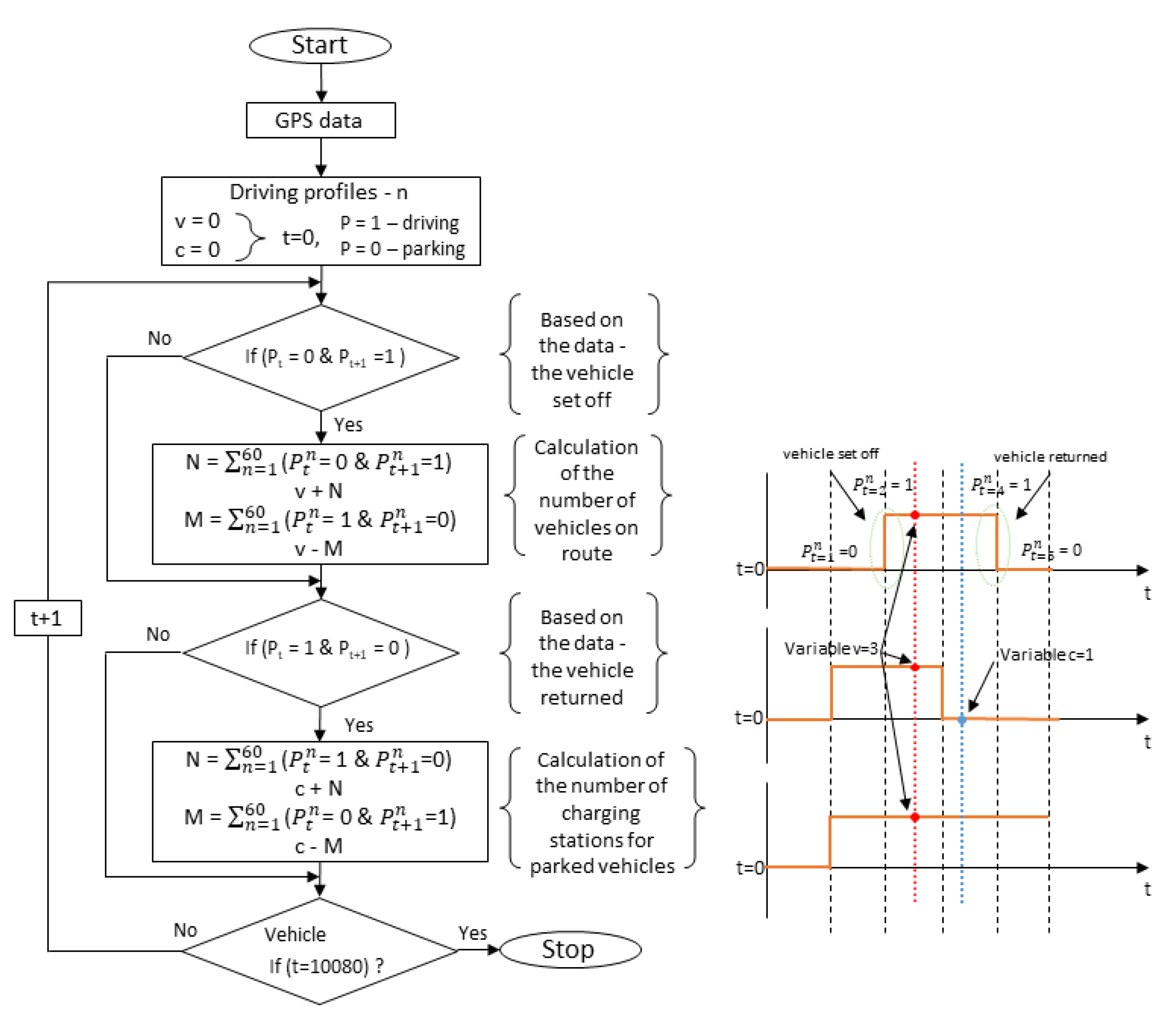
By having routes for 60 vehicles, it is possible to check whether the routes carried out by the fleet can be carried out by a smaller number of vehicles. Accordingly, a concept has been implemented to optimize the required minimum number of vehicles and charging stations that are able to fulfil the requirements defined by the daily profiles of the vehicles. The principle of the algorithm is shown in Figure 14. The results of the algorithm are two values representing the number of vehicles that are on the road at the same time and the number of charging stations that would be sufficient to charge vehicles between routes. The algorithm checks whether the vehicle is on route or parked on company premises for each measurement point. The criterion that must be met is that all routes are completed within the designated intervals according to the profiles recorded.

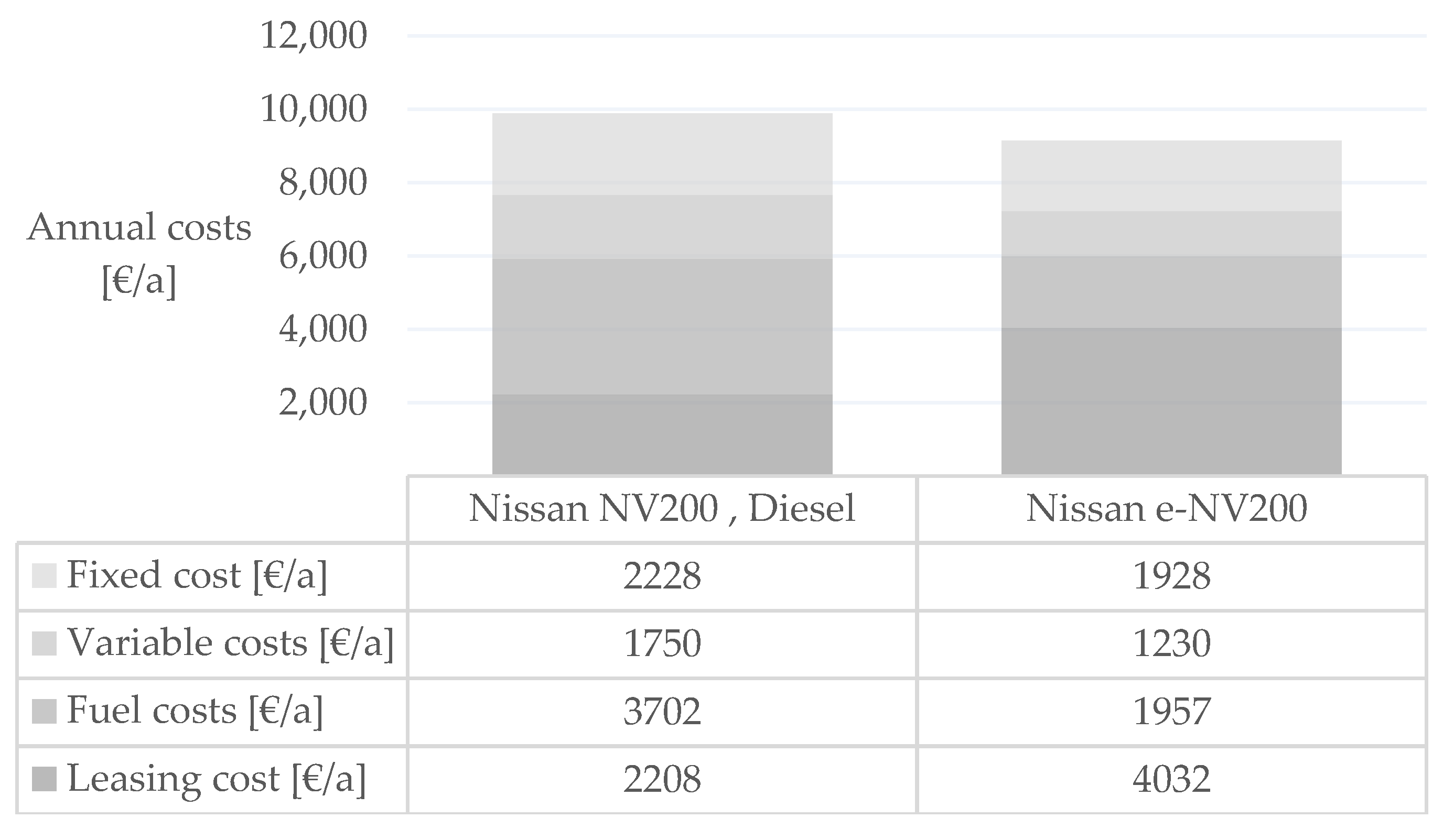
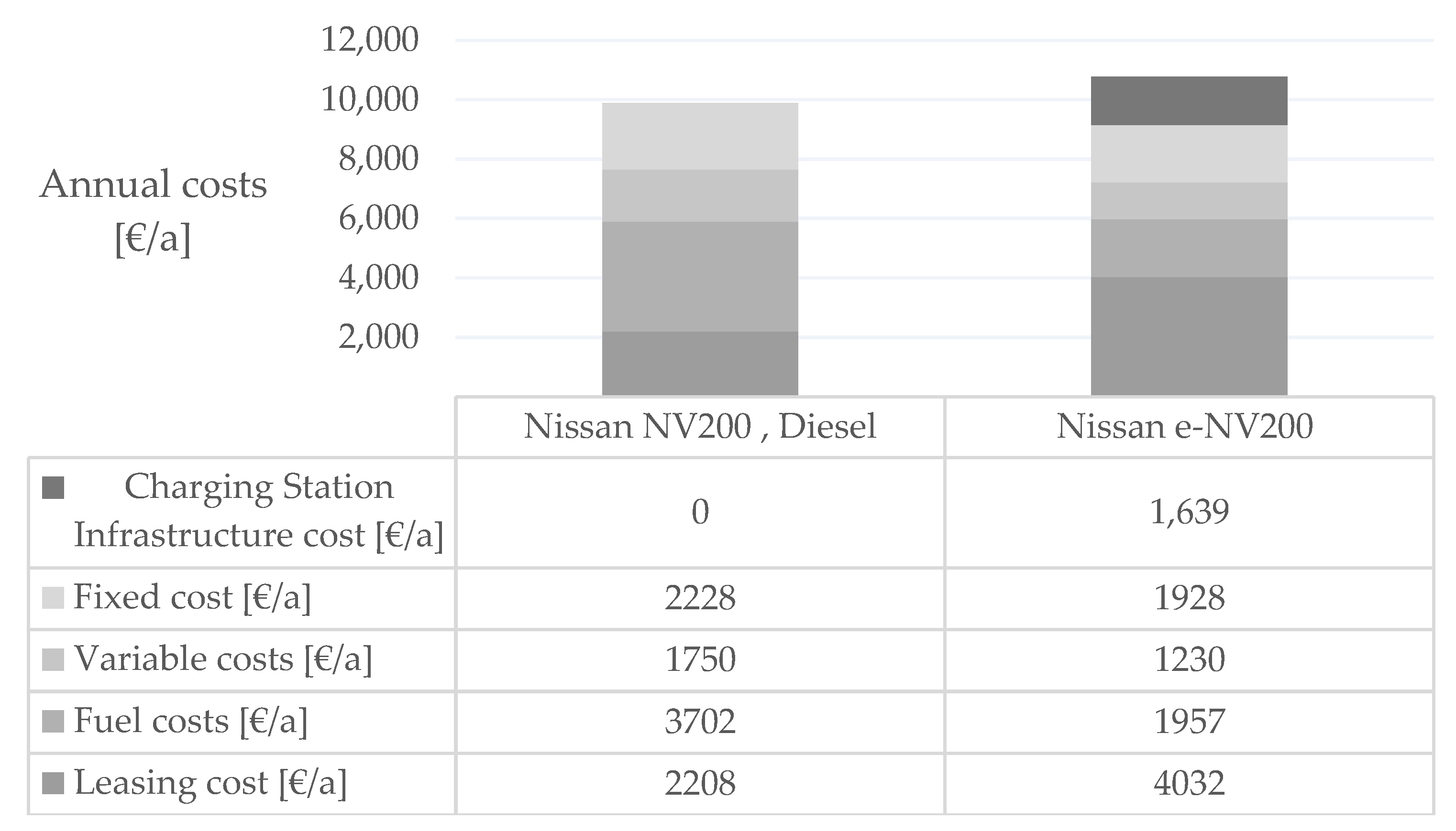
Based on the analysis of 60 profiles, the algorithm reduced the original number of vehicles to 38. In a lot of cases, companies may have a certain number of replacement vehicles, which is not taken into account in this case. The result of 38 also corresponds to the installation of 38 charging stations, assuming that each vehicle is connected to the grid at night. Taking into account the technical and economic analysis carried out, the cost of using both the traditional fleet of ICEVs and EVs was determined. The results are shown in

Table 23. Charging station characteristics [90,91].

Fleet Details	ICEV Fleet	BEV Fleet
Number of fleet vehicles	38	38
Real consumption [L/100 km]	8.91	28.12
CO2 equivalent [ton/a]	614	126
PM10 [kg/a]	52.49	51.26
Fleet TCO [€/a]
Holding time [annual]	5	5
Annual mileage [km/a]	1,140,000	1,140,000
Leasing cost [€/a]	83,904	153,216
Fuel costs [€/a]	140,666	74,365
Variable costs [€/a]	66,500	46,740
Fixed costs [€/a]	84,664	73,264
Charging Station Infrastructure cost [€/a]	0	62,292
SUM [€/a]	375,734	409,877
Annual electricity consumption [MWh/a]		320.54

.

It can be seen that the fleet cost is higher for a fleet of EVs. The biggest impact here is the installation of the charging infrastructure, which is necessary for the proper operation of the BEV fleet. This is, nevertheless, a one-off cost, occurring at the beginning of the investment. As shown in the earlier analysis, costs for the electric fleet decrease over time within a few years of the investment. In addition, a fuel price can be determined for the fleet at which an EV becomes economically preferable. The objective function in this case will take the form ∆TCO ≥ 0.

$${\mathrm{TCO}=\mathrm{TCO}}_{\mathrm{ICE}}\left({\mathrm{C}}_{\mathrm{Diesel}}\right){ - \mathrm{TCO}}_{\mathrm{EV}}\left({\mathrm{C}}_{\mathrm{Electricity}}\right)\ge 0$$

(32)

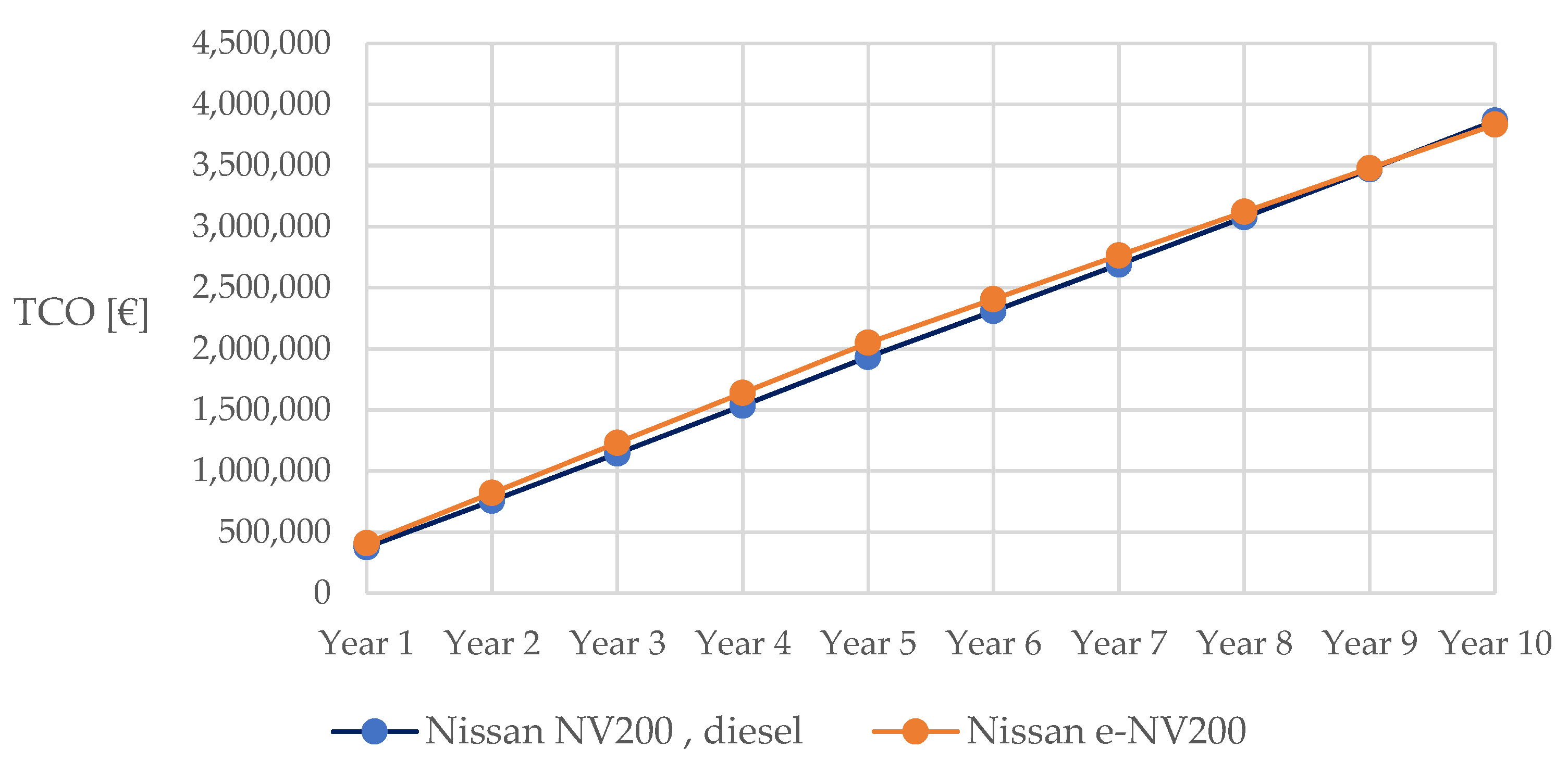
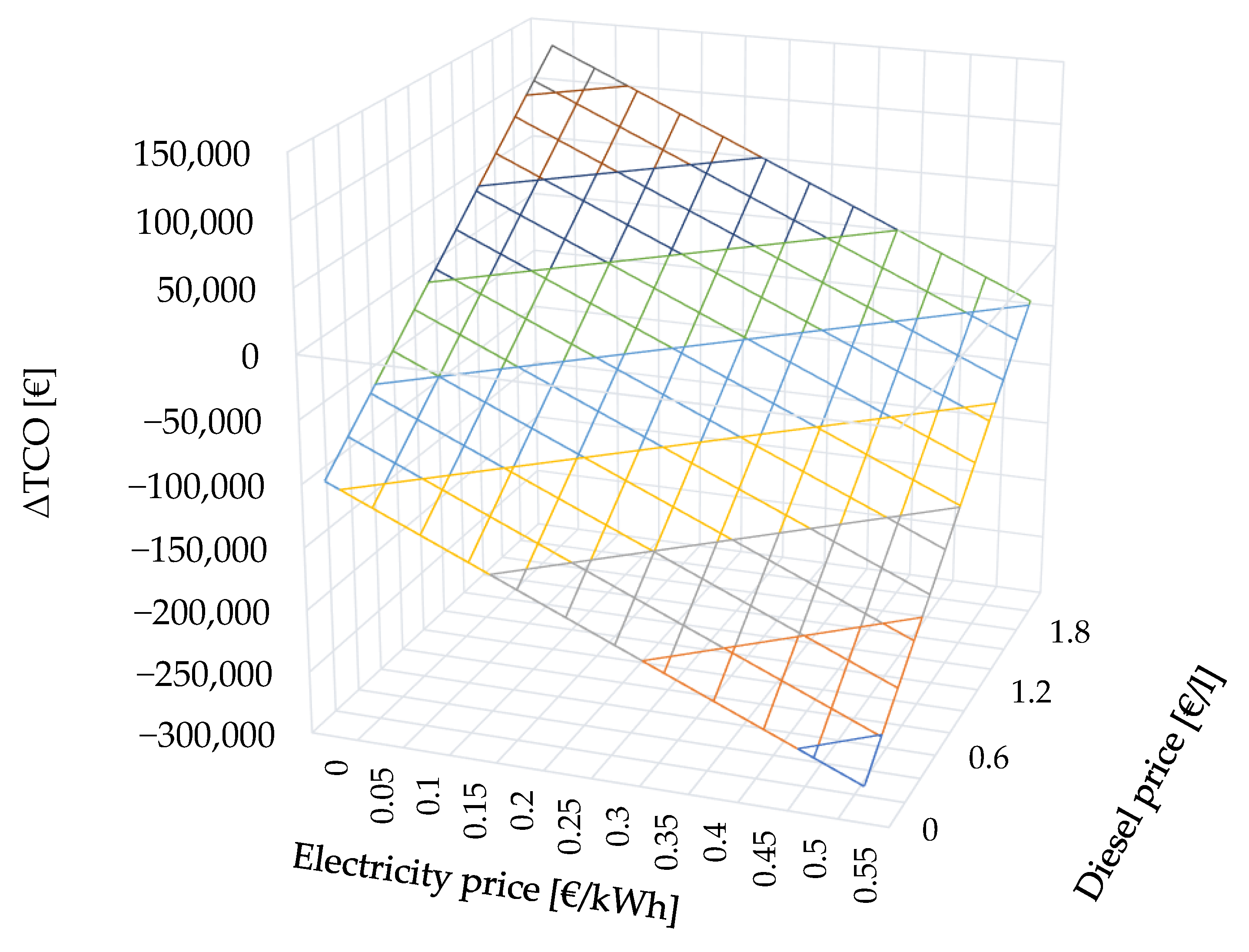
Based on the economic analysis carried out, values were determined for the price of diesel and electricity at which the so-called breakpoint occurs and the use of an EV fleet is profitable. The price of electricity for commercial companies was 21.38 ct/kWh on 1 April 2021 [92]. The price of 1.6 €/L for diesel makes it more cost-effective to use a fleet of EVs. The average diesel price from 1 January to 19 July 2022 was 200.52 ct/L. However, the price of electricity has not remained the same and is now 26.64 ct/kWh for commercial companies [92]. Regarding this price distribution, it is clearly more advantageous to use a fleet of electric vehicles. In this case, the purchase of energy in its entirety from the distributor was considered without taking into account the possibility of reducing energy prices through additional energy storage or renewable sources. The distribution of cost-effectiveness relationships is shown in Figure 15.

5. Conclusions

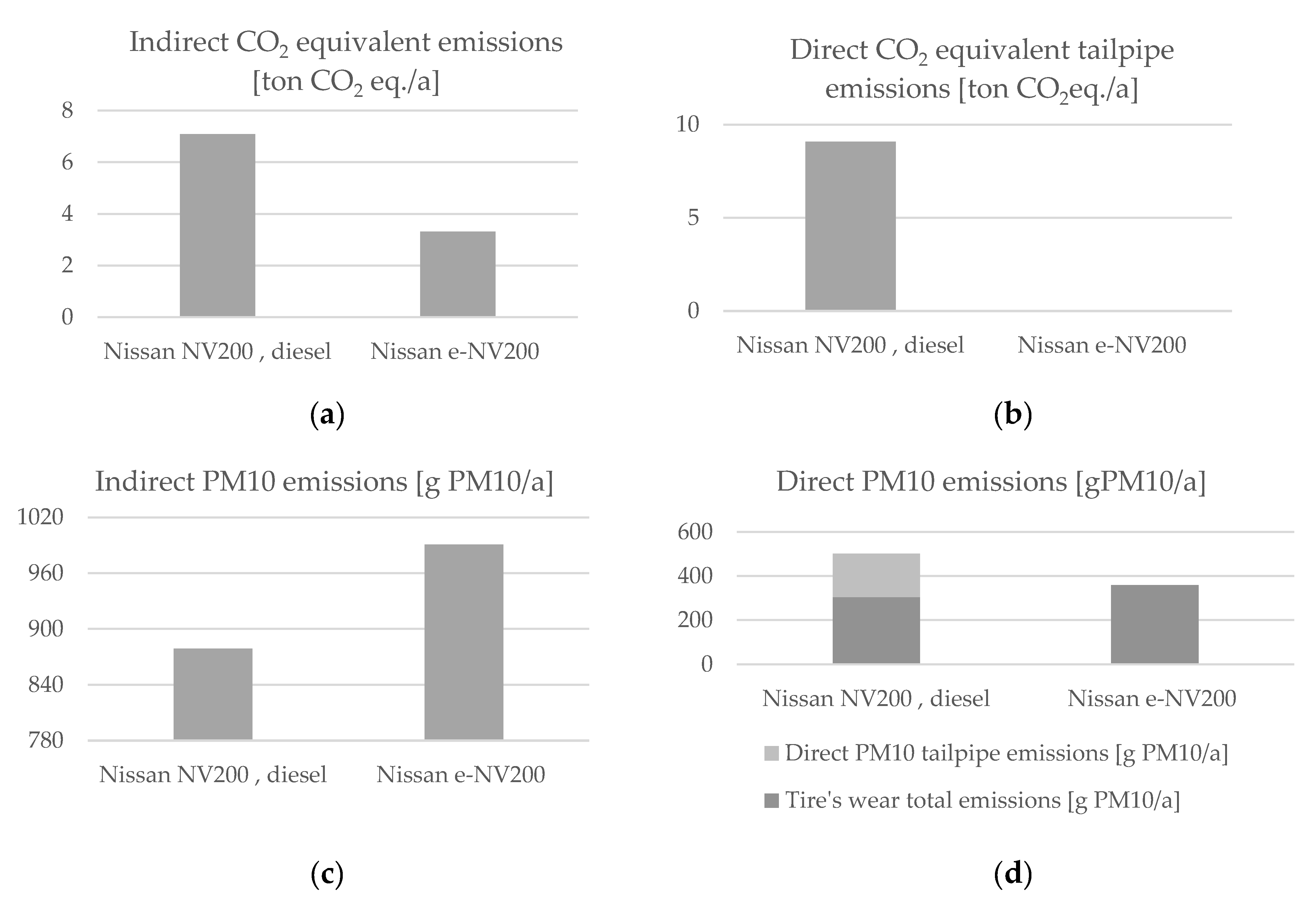
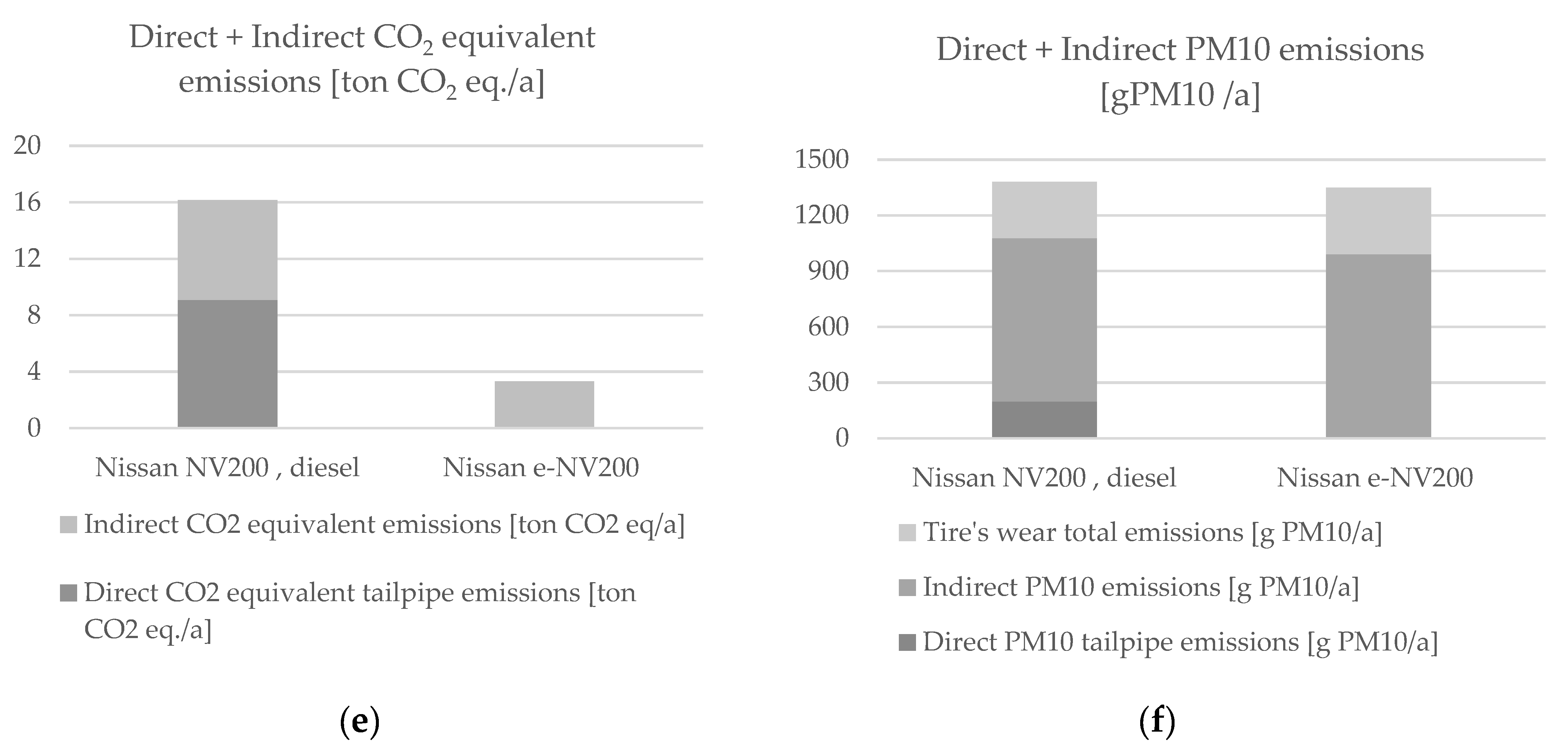
This paper analyses the technical, environmental and economic transformation of a vehicle fleet to reduce atmospheric emissions. Following on from the considerations, assumptions and assessments already discussed, an electric powertrain is suitable for a commercial LDV fleet. However, the EV fleet is a more expensive option and also includes the design and construction of the charging infrastructure; this can be assessed as a disadvantage of the BEV fleet. Moreover, environmentally, the electric LDV fleet results in a considerable reduction (up to 80%) in GHG emissions and a small reduction in PM10 emissions. The PM10 emissions are strongly linked to the national energy mix. CO₂ equivalent emissions are reduced by almost 80%, with major environmental benefits. These values are closely linked to the mix of electricity sources, meaning that if the company were to build its power plant using renewable energy, the emissions associated with its energy production would be zero.

The work presents the conclusions of the analysis on the basis of data, available and reliable from studies, reports and own recorded values. The work is aimed at businesses as an argument for the use of electric vehicles to carry out logistics tasks. For policymakers, it is an argument that the introduced restrictions make sense and the emissions of harmful substances into the atmosphere are gradually reduced. The introduction of other methods that use measurement data can contribute to more precise results that would describe the process more accurately. Nevertheless, the methods presented in this work can be easily implemented in any company and indicate theoretical and practical savings for the company.

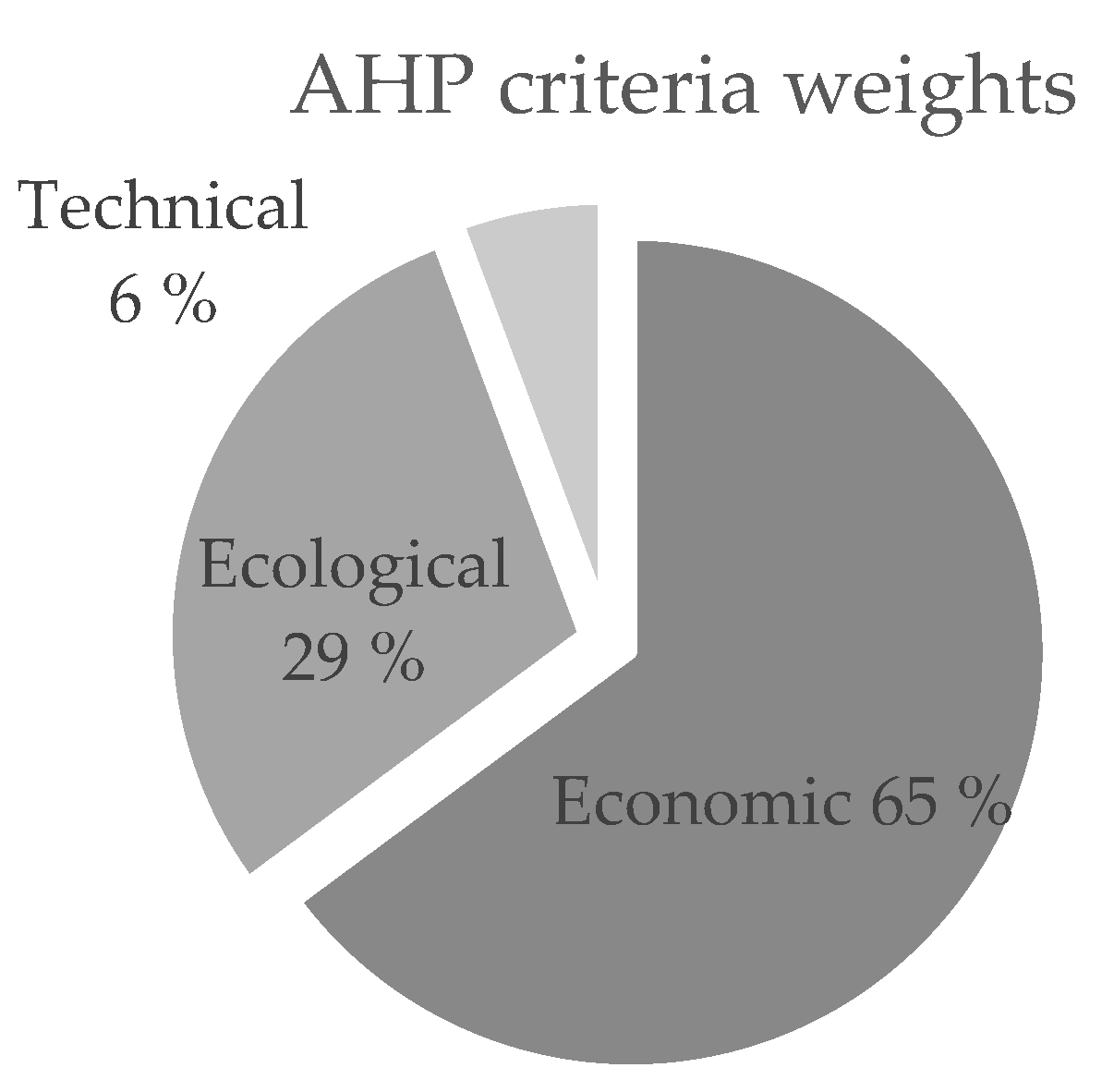
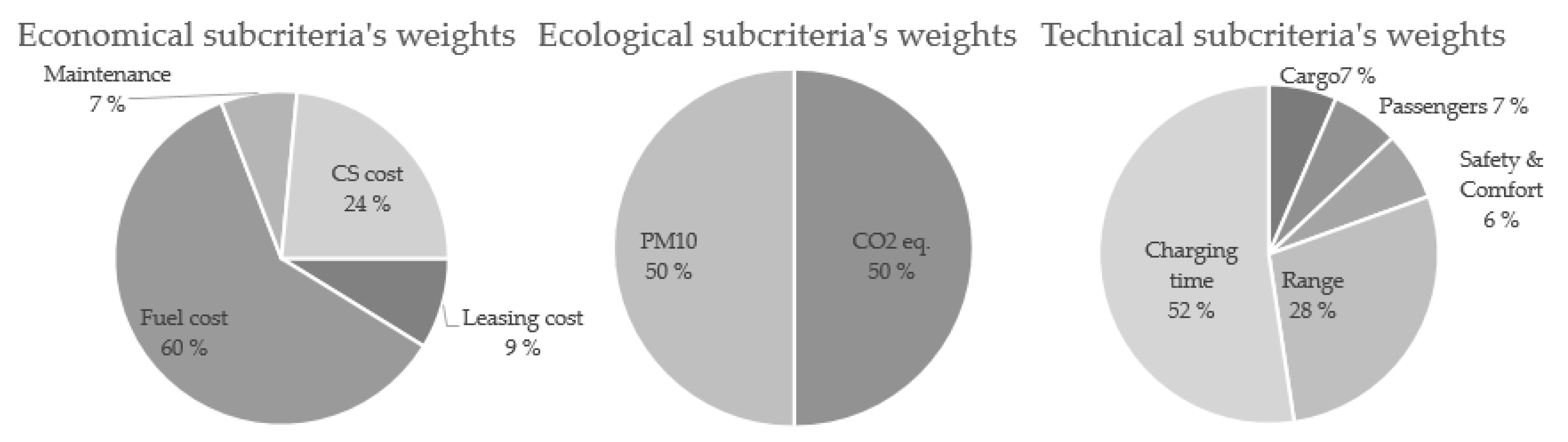
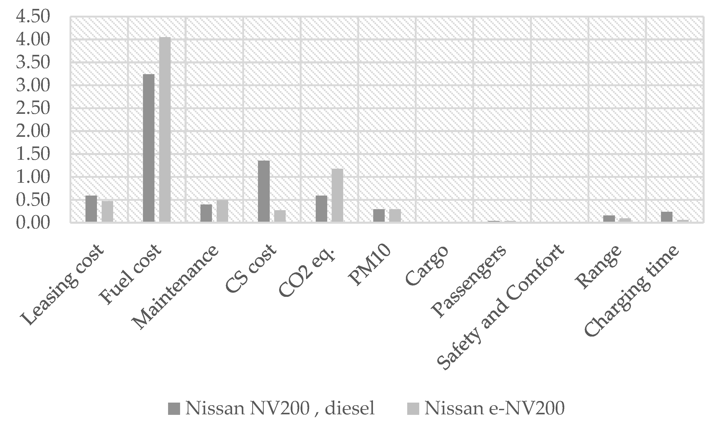
Following the results of the analysis, a hierarchy was proposed between the three criteria analyzed. This hierarchy helps to determine, depending on the needs of the company, which technology reflects their needs. The development of an AHP calculated a score for each alternative, resulting in a higher score for the EV fleet. Considering the increasing importance of the environmental factor, the EV fleet achieves a higher final score. The hypothesis made earlier regarding the hierarchy of the criteria justifies this result: the economic criterion has a higher weighting than the other criteria and, consequently, the sub-criteria.

The BEV fleet fully meets the characteristics required by the vehicle usage profile. The TCO of the electric fleet is higher than that of the conventional fleet due to the infrastructure costs of the charging stations. These costs are spread over a period of five years, after which only the maintenance of the charging stations is taken into account. Once the investment in charging stations has been recouped, the TCO of the electric fleet is lower than that of the conventional fleet.

The company obtains advantages both in terms of economic benefits, special permits for circulation and for the image of company. Employing a fleet of electric LDVs for a logistics company operating in the publishing industry to make and receive deliveries that cover 30,000 km per year has been shown to be an environmentally, economically and technologically beneficial option.

The proposed solution can provide a basis for practical analysis on the basis of real data for other car models and their assessment of compliance with the requirements of new regulations and directives on environmental protection and reduction of harmful emissions. In addition, it can give a basis for preparing a product in the form of an application for commercial use and offering services to enterprises. Eventually, it can also form part of an audit for some specialized companies.

The model is based on values that are included in the lease contract for which prices remain unchanged for the length of the lease. In contrast, the analysis carried out depends heavily on prices, such as fuel and electricity prices, which cannot be considered relatively stable in 2022. It is difficult to predict the behavior of resources prices in the energy market. A possible solution to this problem is to dynamically integrate price volatility into the model. In addition, the model will work more correctly and provide more accurate results if the human factor, i.e., the driver’s driving style and weather conditions, are taken into account. It is advisable to use instantaneous values in the model and to take into account the unit prices of the equipment for the time period considered. The inclusion of random factors, e.g., the failure of a particular vehicle and therefore the inability of the vehicle to meet its targets, is an appropriate implementation to improve the performance of the algorithm. Increasing the frequency of measurement samples recorded during vehicle operation is also a beneficial factor in the results obtained. The model is valid when the input data are updated for a given time period. Further work will focus on increasing the number of parameters affecting vehicle costs and performance.

References

1. Kazak, T. European Green Deal. Yearbook Law Dep. 2022, 9, 304–315. [Google Scholar] [CrossRef]
2. Europrean Commision. EU Open Data Portal; Europrean Commision: Brussels, Belgium, 2020. [Google Scholar]
3. Noel, L.; Zarazua de Rubens, G.; Kester, J.; Sovacool, B.K. Beyond emissions and economics: Rethinking the co-benefits of electric vehicles (EVs) and vehicle-to-grid (V2G). Transp. Policy 2018, 71, 130–137. [Google Scholar] [CrossRef]
4. Pietracho, R.; Wenge, C.; Balischewski, S.; Lombardi, P.; Komarnicki, P.; Kasprzyk, L.; Burzyński, D. Potential of Using Medium Electric Vehicle Fleet in a Commercial Enterprise Transport in Germany on the Basis of Real-World GPS Data. Energies 2021, 14, 5327. [Google Scholar] [CrossRef]
5. Teixeira, A.C.R.; Sodré, J.R. Impacts of replacement of engine powered vehicles by electric vehicles on energy consumption and CO 2 emissions. Transp. Res. Part D Transp. Environ. 2018, 59, 375–384. [Google Scholar] [CrossRef]
6. Ji, S.; Cherry, C.R.; Bechle, M.J.; Wu, Y.; Marshall, J.D. Electric Vehicles in China: Emissions and Health Impacts. Environ. Sci. Technol. 2012, 46, 2018–2024. [Google Scholar] [CrossRef] [PubMed]
7. Ravi, S.S.; Aziz, M. Utilization of Electric Vehicles for Vehicle-to-Grid Services: Progress and Perspectives. Energies 2022, 15, 589. [Google Scholar] [CrossRef]
8. Komarnicki, P.; Haubrock, J.; Styczynski, Z.A. Elektromobilität und Sektorenkopplung; Springer: Berlin/Heidelberg, Germany, 2020; ISBN 978-3-662-62035-9. [Google Scholar]
9. Komarnicki, P.; Wenge, C.; Pietracho, R. Electromobility—Integration of electric vehicles with the power grid infrastructure. Prz. Elektrotechniczny 2020, 96, 3–15. [Google Scholar] [CrossRef]
10. Martínez-Lao, J.; Montoya, F.G.; Montoya, M.G.; Manzano-Agugliaro, F. Electric vehicles in Spain: An overview of charging systems. Renew. Sustain. Energy Rev. 2017, 77, 970–983. [Google Scholar] [CrossRef]
11. Wenge, C.; Komarnicki, P.; Styczynski, Z.A. Models and boundaries of data exchange between electric-vehicle and charging-point. Example of a practical realisation. In Proceedings of the 2010 Modern Electric Power Systems, Wroclaw, Poland, 20–22 September 2010; pp. 1–4. [Google Scholar]
12. Burzyński, D.; Głuchy, D.; Godek, M. Analysis of the impact of quick charge technology on the charging process parameters of the lithium-ion storage at various temperatures. ITM Web Conf. 2018, 19, 01035. [Google Scholar] [CrossRef] [Green Version]
13. Helm, S.; Hauer, I.; Wolter, M.; Wenge, C.; Balischewski, S.; Komarnicki, P. Impact of unbalanced electric vehicle charging on low-voltage grids. In Proceedings of the 2020 IEEE PES Innovative Smart Grid Technologies Europe (ISGT-Europe), Hague, The Netherlands, 26–28 October 2020; IEEE: Manhattan, NY, USA, 2020; pp. 665–669. [Google Scholar]
14. Wenge, C.; Guo, H.; Roehrig, C. Measurement-based harmonic current modeling of mobile storage for power quality study in the distribution system. Arch. Electr. Eng. 2017, 66, 801–814. [Google Scholar] [CrossRef]
15. Chen, F.; Chen, Z.; Dong, H.; Yin, Z.; Wang, Y.; Liu, J. Research on the Influence of Electric Vehicle Multi-Factor Charging Load on a Regional Power Grid. In Proceedings of the 2018 10th International Conference on Measuring Technology and Mechatronics Automation (ICMTMA), Changsha, China, 10–11 February 2018; IEEE: Manhattan, NY, USA, 2018; pp. 163–166. [Google Scholar]
16. Fan, Y.; Guo, C.; Hou, P.; Tang, Z. Impact of Electric Vehicle Charging on Power Load Based on TOU Price. Energy Power Eng. 2013, 05, 1347–1351. [Google Scholar] [CrossRef]
17. Kasprzyk, L.; Domeracka, A.; Burzyński, D. Modelling of lithium-ion batteries operation and life in electric vehicles. Prz. Elektrotechniczny 2018, 94, 158–161. [Google Scholar] [CrossRef]
18. Ioakimidis, C.S.; Thomas, D.; Rycerski, P.; Genikomsakis, K.N. Peak shaving and valley filling of power consumption profile in non-residential buildings using an electric vehicle parking lot. Energy 2018, 148, 148–158. [Google Scholar] [CrossRef]
19. Khan, S.U.; Mehmood, K.K.; Haider, Z.M.; Rafique, M.K.; Khan, M.O.; Kim, C.-H. Coordination of Multiple Electric Vehicle Aggregators for Peak Shaving and Valley Filling in Distribution Feeders. Energies 2021, 14, 352. [Google Scholar] [CrossRef]
20. Wenge, C.; Pietracho, R.; Balischewski, S.; Arendarski, B.; Lombardi, P.; Komarnicki, P.; Kasprzyk, L. Multi Usage Applications of Li-Ion Battery Storage in a Large Photovoltaic Plant: A Practical Experience. Energies 2020, 13, 4590. [Google Scholar] [CrossRef]
21. Li, X.; Tan, Y.; Liu, X.; Liao, Q.; Sun, B.; Cao, G.; Li, C.; Yang, X.; Wang, Z. A cost-benefit analysis of V2G electric vehicles supporting peak shaving in Shanghai. Electr. Power Syst. Res. 2020, 179, 106058. [Google Scholar] [CrossRef]
22. Babaei, M.; Azizi, E.; Beheshti, M.T.; Hadian, M. Data-Driven load management of stand-alone residential buildings including renewable resources, energy storage system, and electric vehicle. J. Energy Storage 2020, 28, 101221. [Google Scholar] [CrossRef]
23. Hajebrahimi, A.; Kamwa, I.; Huneault, M. A novel approach for plug-in electric vehicle planning and electricity load management in presence of a clean disruptive technology. Energy 2018, 158, 975–985. [Google Scholar] [CrossRef]
24. Chung, Y.-W.; Khaki, B.; Li, T.; Chu, C.; Gadh, R. Ensemble machine learning-based algorithm for electric vehicle user behavior prediction. Appl. Energy 2019, 254, 113732. [Google Scholar] [CrossRef]
25. Apostolaki-Iosifidou, E.; Codani, P.; Kempton, W. Measurement of power loss during electric vehicle charging and discharging. Energy 2017, 127, 730–742. [Google Scholar] [CrossRef]
26. Crozier, C.; Deakin, M.; Morstyn, T.; McCulloch, M. Coordinated electric vehicle charging to reduce losses without network impedances. IET Smart Grid 2020, 3, 677–685. [Google Scholar] [CrossRef]
27. Zhang, W.; Spence, K.; Shao, R.; Chang, L. Optimal Scheduling of Spinning Reserve and User Cost in Vehicle-to-Grid (V2G) Systems. In Proceedings of the 2018 IEEE Energy Conversion Congress and Exposition (ECCE), Portland, OR, USA, 23–27 September 2018; IEEE: Manhattan, NY, USA, 2018; pp. 1058–1064. [Google Scholar]
28. Rahmani-andebili, M. Spinning reserve supply with presence of electric vehicles aggregator considering compromise between cost and reliability. IET Gener. Transm. Distrib. 2013, 7, 1442–1452. [Google Scholar] [CrossRef]
29. Singh, S.; Jagota, S.; Singh, M. Energy management and voltage stabilization in an islanded microgrid through an electric vehicle charging station. Sustain. Cities Soc. 2018, 41, 679–694. [Google Scholar] [CrossRef]
30. Khan, A.; Memon, S.; Sattar, T.P. Analyzing Integrated Renewable Energy and Smart-Grid Systems to Improve Voltage Quality and Harmonic Distortion Losses at Electric-Vehicle Charging Stations. IEEE Access 2018, 6, 26404–26415. [Google Scholar] [CrossRef]
31. Codani, P.; Petit, M.; Perez, Y. Participation of an electric vehicle fleet to primary frequency control in France. Int. J. Electr. Hybrid Veh. 2015, 7, 233. [Google Scholar] [CrossRef]
32. Janjic, A.; Velimirovic, L.; Stankovic, M.; Petrusic, A. Commercial electric vehicle fleet scheduling for secondary frequency control. Electr. Power Syst. Res. 2017, 147, 31–41. [Google Scholar] [CrossRef]
33. Naveed, A.; Sonmez, Ş.; Ayasun, S. Impact of Electric Vehicle Aggregator with Communication Time Delay on Stability Regions and Stability Delay Margins in Load Frequency Control System. J. Mod. Power Syst. Clean Energy 2021, 9, 595–601. [Google Scholar] [CrossRef]
34. Iqbal, S.; Xin, A.; Jan, M.U.; ur Rehman, H.; Masood, A.; Abbas Rizvi, S.A.; Salman, S. Aggregated Electric Vehicle-to-Grid for Primary Frequency Control in a Microgrid- A Review. In Proceedings of the 2018 IEEE 2nd International Electrical and Energy Conference (CIEEC), Beijing, China, 4–6 November 2018; IEEE: Manhattan, NY, USA, 2018; pp. 563–568. [Google Scholar]
35. Gielen, D.; Boshell, F.; Saygin, D.; Bazilian, M.D.; Wagner, N.; Gorini, R. The role of renewable energy in the global energy transformation. Energy Strateg. Rev. 2019, 24, 38–50. [Google Scholar] [CrossRef]
36. Joas, F.; Pahle, M.; Flachsland, C.; Joas, A. Which goals are driving the Energiewende? Making sense of the German Energy Transformation. Energy Policy 2016, 95, 42–51. [Google Scholar] [CrossRef]
37. Wilson, C.; Tyfield, D. Critical perspectives on disruptive innovation and energy transformation. Energy Res. Soc. Sci. 2018, 37, 211–215. [Google Scholar] [CrossRef]
38. Xing, Z.; Zhu, J.; Zhang, Z.; Qin, Y.; Jia, L. Energy consumption optimization of tramway operation based on improved PSO algorithm. Energy 2022, 258, 124848. [Google Scholar] [CrossRef]
39. Xing, Z.; Zhang, Z.; Guo, J.; Qin, Y.; Jia, L. Rail train operation energy-saving optimization based on improved brute-force search. Appl. Energy 2023, 330, 120345. [Google Scholar] [CrossRef]
40. Zhang, Z.; Zhang, H.; Zhou, L. Zero-carbon measure prioritization for sustainable freight transport using interval 2 tuple linguistic decision approaches. Appl. Soft Comput. 2023, 132, 109864. [Google Scholar] [CrossRef]
41. Brown, T.; Schlachtberger, D.; Kies, A.; Schramm, S.; Greiner, M. Synergies of sector coupling and transmission reinforcement in a cost-optimised, highly renewable European energy system. Energy 2018, 160, 720–739. [Google Scholar] [CrossRef] [Green Version]
42. Fridgen, G.; Keller, R.; Körner, M.-F.; Schöpf, M. A holistic view on sector coupling. Energy Policy 2020, 147, 111913. [Google Scholar] [CrossRef]
43. Ramsebner, J.; Haas, R.; Ajanovic, A.; Wietschel, M. The sector coupling concept: A critical review. WIREs Energy Environ. 2021, 10. [Google Scholar] [CrossRef]
44. Alalewi, A.; Dayoub, I.; Cherkaoui, S. On 5G-V2X Use Cases and Enabling Technologies: A Comprehensive Survey. IEEE Access 2021, 9, 107710–107737. [Google Scholar] [CrossRef]
45. Husain, S.S.; Kunz, A.; Prasad, A.; Pateromichelakis, E.; Samdanis, K. Ultra-High Reliable 5G V2X Communications. IEEE Commun. Stand. Mag. 2019, 3, 46–52. [Google Scholar] [CrossRef]
46. Sharma, V.; You, I.; Guizani, N. Security of 5G-V2X: Technologies, Standardization, and Research Directions. IEEE Netw. 2020, 34, 306–314. [Google Scholar] [CrossRef]
47. Burzyński, D.; Kasprzyk, L. A novel method for the modeling of the state of health of lithium-ion cells using machine learning for practical applications. Knowledge-Based Syst. 2021, 219, 106900. [Google Scholar] [CrossRef]
48. Senn-Kalb, L.; Mehta, D. eMobility—Market Insights & Data Analysis, Statista. 2021. Available online: https://www.statista.com/study/49240/emobility---market-insights-and-data-analysis/ (accessed on 1 December 2022).
49. Bernhart, W. Wertschöpfung steigern mit Battery-as-a-Service. ATZextra 2020, 25, 14–19. [Google Scholar] [CrossRef]
50. Tahara, K.; Ishikawa, K.; Ishigaki, M. Battery as a Service for Electric Vehicles: Design and Optimization of Partially Swappable and Shareable Battery System. In Proceedings of the 2020 IEEE 23rd International Conference on Intelligent Transportation Systems (ITSC), Rhodes, Greece, 20–23 September 2020; IEEE: Manhattan, NY, USA, 2020; pp. 1–8. [Google Scholar]
51. Shi, L.; Hu, B. Battery as a Service: Flexible Electric Vehicle Battery Leasing. SSRN Electron. J. 2022. [Google Scholar] [CrossRef]
52. IEA. Global EV Outlook 2021. Accelerating Ambitions Despite the Pandemic. Available online: https://iea.blob.core.windows.net/assets/ed5f4484-f556-4110-8c5c-4ede8bcba637/GlobalEVOutlook2021.pdf (accessed on 1 December 2022).
53. IEA. Worldwide Number of Battery Electric Vehicles in Use from 2016 to 2020 (in millions), Statista. 2021. Available online: https://www.statista.com/statistics/270603/worldwide-number-of-hybrid-and-electric-vehicles-since-2009/ (accessed on 1 December 2022).
54. KBA, Anzahl der Lastkraftwagen in Deutschland von 1960 bis 2022, Statista. 2022. Available online: https://de.statista.com/statistik/daten/studie/6961/umfrage/anzahl-der-lkw-in-deutschland (accessed on 1 December 2022).
55. Weltweiter Absatz von Kraftfahrzeugen nach Fahrzeugtyp von 2016 bis 2021, Statista. Available online: https://de.statista.com/statistik/daten/studie/1255787/umfrage/kfz-absatz-weltweit-nach-fahrzeugtyp/ (accessed on 1 December 2022).
56. Juan, A.; Mendez, C.; Faulin, J.; de Armas, J.; Grasman, S. Electric Vehicles in Logistics and Transportation: A Survey on Emerging Environmental, Strategic, and Operational Challenges. Energies 2016, 9, 86. [Google Scholar] [CrossRef] [Green Version]
57. Dörr, N.; Dorrmann, L.; Klebsch, W.O.A. Logistik, Energie und Mobilität 2030, Bundeswirtschaftsministerium. 2020. Available online: https://www.vde.com/resource/blob/2013758/3e6f90ce5a2bf8baee20f0056bc4f3b9/studie-logistik-mobilitaet-und-energie-2030-data.pdf (accessed on 1 December 2022).
58. Ashfaq, M.; Butt, O.; Selvaraj, J.; Rahim, N. Assessment of electric vehicle charging infrastructure and its impact on the electric grid: A review. Int. J. Green Energy 2021, 18, 657–686. [Google Scholar] [CrossRef]
59. Gonzalez Venegas, F.; Petit, M.; Perez, Y. Active integration of electric vehicles into distribution grids: Barriers and frameworks for flexibility services. Renew. Sustain. Energy Rev. 2021, 145, 111060. [Google Scholar] [CrossRef]
60. Rivera, S.; Kouro, S.; Vazquez, S.; Goetz, S.M.; Lizana, R.; Romero-Cadaval, E. Electric Vehicle Charging Infrastructure: From Grid to Battery. IEEE Ind. Electron. Mag. 2021, 15, 37–51. [Google Scholar] [CrossRef]
61. Sokolnikova, P.; Lombardi, P.; Arendarski, B.; Suslov, K.; Pantaleo, A.M.; Kranhold, M.; Komarnicki, P. Net-zero multi-energy systems for Siberian rural communities: A methodology to size thermal and electric storage units. Renew. Energy 2020, 155, 979–989. [Google Scholar] [CrossRef]
62. Lombardi, P.; Sokolnikova, T.; Suslov, K.; Voropai, N.; Styczynski, Z.A. Isolated power system in Russia: A chance for renewable energies? Renew. Energy 2016, 90, 532–541. [Google Scholar] [CrossRef]
63. Churchman, C.W.; Ackoff, R.L. An Approximate Measure of Value. J. Oper. Res. Soc. Am. 1954, 2, 172–187. [Google Scholar] [CrossRef]
64. Olson, D.L. Smart. In Decision Aids for Selection Problems; Springer: New York, NY, USA, 1996; pp. 34–48. [Google Scholar]
65. Saaty, R.W. The analytic hierarchy process—What it is and how it is used. Math. Model. 1987, 9, 161–176. [Google Scholar] [CrossRef]
66. Olson, D.L.; Fliedner, G.; Currie, K. Comparison of the REMBRANDT system with analytic hierarchy process. Eur. J. Oper. Res. 1995, 82, 522–539. [Google Scholar] [CrossRef]
67. Kadoić, N.; Ređep, N.B.; Divjak, B. Decision making with the analytic network process. In Proceedings of the 14th International Symposium on Operational Research, Bled, Slovenia, 27–29 September 2017; pp. 180–186. [Google Scholar] [CrossRef]
68. Figueira, J.R.; Mousseau, V.; Roy, B. ELECTRE Methods. In Multiple Criteria Decision Analysis; Springer: New York, NY, USA, 2016; pp. 155–185. [Google Scholar]
69. Olson, D.L. Multi-Criteria Decision Support. In Handbook on Decision Support Systems 1; Springer Berlin Heidelberg: Berlin, Heidelberg, 2008; pp. 299–314. [Google Scholar]
70. Zhang, Z.; Guo, J.; Zhang, H.; Zhou, L.; Wang, M. Product selection based on sentiment analysis of online reviews: An intuitionistic fuzzy TODIM method. Complex Intell. Syst. 2022, 8, 3349–3362. [Google Scholar] [CrossRef]
71. Franek, J.; Kresta, A. Judgment Scales and Consistency Measure in AHP. Procedia Econ. Financ. 2014, 12, 164–173. [Google Scholar] [CrossRef] [Green Version]
72. Pavlovic, J.; Marotta, A.; Ciuffo, B. CO2 emissions and energy demands of vehicles tested under the NEDC and the new WLTP type approval test procedures. Appl. Energy 2016, 177, 661–670. [Google Scholar] [CrossRef]
73. Rangaraju, S.; De Vroey, L.; Messagie, M.; Mertens, J.; Van Mierlo, J. Impacts of electricity mix, charging profile, and driving behavior on the emissions performance of battery electric vehicles: A Belgian case study. Appl. Energy 2015, 148, 496–505. [Google Scholar] [CrossRef]
74. German Electricity Mix: Electricity Generation Germany Until 2022. Available online: https://strom-report.de/strom/ (accessed on 1 December 2022).
75. International Panel Climate Change Global Warming Potential Values. Available online: www.ipcc.ch%0Aghgprotocol.org/.../Global-Warming-Potential-Values (accessed on 16 February 2016).
76. Brook, J.R.; Dann, T.F.; Burnett, R.T. The Relationship Among TSP, PM 10, PM 2.5, and Inorganic Constituents of Atmospheric Participate Matter at Multiple Canadian Locations. J. Air Waste Manage. Assoc. 1997, 47, 2–19. [Google Scholar] [CrossRef] [Green Version]
77. Turconi, R.; Boldrin, A.; Astrup, T. Life cycle assessment (LCA) of electricity generation technologies: Overview, comparability and limitations. Renew. Sustain. Energy Rev. 2013, 28, 555–565. [Google Scholar] [CrossRef] [Green Version]
78. Trozzi, C.; Nielsen, O.-K.; Plejdrup, M.; Rentz, O.; Oertel, D.; Woodfield, M.; Stewart, R. EMEP/EEA Air Pollutant Emission Inventory Guidebook 2019; European Environment Agency: Copenhagen, Denmark, 2019. [Google Scholar]
79. Wissenschaftliche Dienste. CO2-Emissionen im Verkehrsbereich. 2019. Available online: https://www.bundestag.de/resource/blob/660794/dfdee26b00e44b018b04a187f0c6843e/WD-8-056-19-pdf-data.pdf (accessed on 1 December 2022).
80. WMO and UNEP, Climate Change 2021—The Physical Science Basis 2021, The Intergovernmental Panel on Climate Change. 2022. Available online: https://www.ipcc.ch/report/sixth-assessment-report-working-group-i/ (accessed on 1 December 2022).
81. Vanherle, K.; Lopez-Aparicio, S.; Grythe, H.; Lükewille, A.; Unterstaller, A.; Mayeres, I. Transport Non-Exhaust PM-Emissions—An Overview of Emission Estimates, Relevance, Trends and Policies; European Commission: Luxembourg, 2021. [Google Scholar]
82. Commission, E. CO₂ Emission Performance Standards for Cars and Vans; European Commission: Luxembourg, 2021. [Google Scholar]
83. Vehicle tax calculator for Germany. Available online: https://kfz-steuer.wiki/en/ (accessed on 1 December 2022).
84. Hauff, K.; Pfahl, S.; Degenkolb, R. Taxation of Electric Vehicles in Europe: A Methodology for Comparison. World Electr. Veh. J. 2018, 9, 30. [Google Scholar] [CrossRef] [Green Version]
85. Own data. Cost of IFF Electric Car Insurance. 2019.
86. Electric Power Research Institute. Total Cost of Ownership Model for Current Plug-in Electric Vehicles; Electric Power Research Institute: Palo Alto, CA, USA, 2013. [Google Scholar]
87. Propfe, B.; Redelbach, M.; Santini, D.; Friedrich, H. Cost analysis of Plug-in Hybrid Electric Vehicles including Maintenance & Repair Costs and Resale Values. World Electr. Veh. J. 2012, 5, 886–895. [Google Scholar] [CrossRef]
88. Logtenberg, R.; Pawley, J.; Saxifrage, B. Comparing Fuel and Maintenance Costs of Electric and Gas Powered Vehicles in Canada; 2 Degrees Institute: Sechelt, BC, Canada, 2018. [Google Scholar]
89. Diesel Average Price in Germany. Available online: https://www.statista.com/statistics/1330032/diesel-average-price-germany/ (accessed on 6 December 2022).
90. Wirtschaftsprüfungsgesellschaft, D.D.G. E-Mobility Ladeinfrastruktur als Geschäftsfeld. 2018. Available online: https://www2.deloitte.com/content/dam/Deloitte/de/Documents/risk/Risk-Deloitte-Ladeinfrastruktur.pdf (accessed on 6 December 2022).
91. der Maur, A.A.; Brüggeshemke, N.; Kutschera, M. Lade-Report Entwicklung der Öffentlich Zugänglichen Ladeinfrastruktur für die Elektromobilität Sowie Vergleich der Ladetarife in Deutschland. 2022. Available online: https://www.prognos.com/sites/default/files/2021-01/20200207_prognos_lade-report_2020.pdf (accessed on 6 December 2022).
92. Electricity Prices for Commercial and Industrial Customers in Germany from 2011 to 2021 (in euro cents per kilowatt hour) Statistical Data. 2022. Available online: https://www.statista.com/statistics/1346782/electricity-prices-commercial-industrial-customers-germany/ (accessed on 1 December 2022).
Figure 1. Worldwide number of battery electric vehicles (BEVs) in use from 2016 to 2021 [53].
Energies 16 00462 g001
Figure 2. The process of the transport of goods from the producer to the consumer [57].
Energies 16 00462 g002
Figure 3. Example of a profile for an EV with indication of the charging time and number of trips.
Energies 16 00462 g003
Figure 4. Life cycle emissions of GHGs and air pollutants from different electricity generation sources [73].
Energies 16 00462 g004
Figure 5. AHP criteria.
Energies 16 00462 g005
Figure 6. AHP criteria normalized weights.
Energies 16 00462 g006
Figure 7. AHP subcriteria’s weights.
Energies 16 00462 g007
Figure 8. Sub-criteria’s score for each car.
Energies 16 00462 g008
Figure 9. Emissions according to analysis for an ICEV and a BEV; (a) indirect CO2 equivalent emissions; (b) direct CO2 equivalent tailpipe emissions; (c) indirect PM10 emissions; (d) direct PM10 emissions; (e) total CO2 emissions; (f) total PM10 emissions.
Energies 16 00462 g009aEnergies 16 00462 g009b
Figure 10. Cost comparison between ICEV and BEV car models at 30,000 [km/a].
Energies 16 00462 g010
Figure 11. TCO costs for an ICEV and a BEV including charging infrastructure cost at 30,000 [km/annual].
Energies 16 00462 g011
Figure 12. TCO costs for an ICEV and a BEV including charging infrastructure cost.
Energies 16 00462 g012
Figure 13. Example of one route taken by a vehicle from the fleet.
Energies 16 00462 g013
Figure 14. Block diagram of the algorithm implemented.
Energies 16 00462 g014
Figure 15. Cost-effectiveness relationships when electricity and diesel fuel prices vary.
Energies 16 00462 g015