Abstract
Integrated optimization of well placement and hydraulic fracture parameters in naturally fractured shale gas reservoirs is of significance to enhance unconventional hydrocarbon energy resources in the oil and gas industry. However, the optimization task usually presents intensive computation-cost due to numerous high-fidelity model simulations, particularly for field-scale application. We present an efficient multi-objective optimization framework supported by a novel hierarchical surrogate-assisted evolutionary algorithm and multi-fidelity modeling technology. In the proposed framework, both the net present value (NPV) and cumulative gas production (CGP) are regarded as the bi-objective functions that need to be optimized. The hierarchical surrogate-assisted evolutionary algorithm employs a novel multi-fidelity particle-swarm optimization of a global–local hybridization searching strategy where the low-fidelity surrogate model is capable of exploring the populations globally, while the high-fidelity models update the current populations and thus generate the next generations locally. The multi-layer perception is chosen as a surrogate model in this study. The performance of our proposed hierarchical surrogate-assisted global optimization approach is verified to optimize the well placement and hydraulic fracture parameters on a hydraulically fractured shale gas reservoir. The proposed surrogate model can obtain both the NPV and CPG with satisfactory accuracy with only 500 training samples. The surrogate model significantly contributes to the convergent performance of multi-objective optimization algorithm.
1. Introduction
Unconventional oil and gas reservoirs, such as shale oil and gas reservoirs and tight oil and gas reservoirs, have become very important oil and gas resources with great potential for exploitation [1]. Unconventional oil and gas reservoirs are characterized by low permeability and strong heterogeneity, so it is almost impossible to obtain productivity without fracturing measures [2]. For the development of such oil and gas reservoirs, most of the major oilfields adopt multi-stage fracturing technology, which can form a complex fracture network, thereby improving the seepage characteristics and increasing the oil/gas resources recovery [3,4]. At present, the hydraulic fracturing technology has been widely used in Bakken, Montney, Eagle Ford, Barnett, Weiyuan, Changning and other regions, and has achieved remarkable development results [5,6,7,8]. However, the fracture morphology is very complex and the flow characteristics are not clear, which increases the difficulty of production prediction and fracturing optimization [9,10].
The optimization of fracture parameters and well pattern in shale gas reservoir development is a maximization problem [11,12,13]. Yong et al. established a seepage mathematical model and an ideal geological model of shale gas reservoir considering slippage effect, solved them by numerical simulation method, and analyzed the influence of fracture number, fracture length and fracture spacing on well productivity [14]. This model then can be used for fracture parameter optimization. Balan et al. analyzed the influence of fracture length, conductivity and fracture spacing of fracturing induced fractures on shale gas well production, and constructed a set of optimal fracturing scheme design processes based on a Lagrange multiplier function [15]. Yu et al. used a semi-analytical method to solve the model, simulate the full life cycle production performance of a multi-well development platform, analyze the impact of various factors on production effect, and optimize the well spacing, fracture spacing and fracture length under different fracturing scales [16]. Rammay et al. proposed a stochastic optimization framework to achieve parameters such as fracture length, conductivity and number of fracturing sections in shale gas reservoirs [17]. Wang et al. simulated the change rule of fracture width with cluster spacing and the change rule of fracture length with sand ratio and sand paving concentration by using 2D and 3D fracture models for an Eagle Ford shale reservoir, and simulated the stress distribution when each parameter changes, which can be used to optimize the perforation cluster spacing [18]. Xiao et al. proposed a machine-learning-based framework to optimize the fracture parameters, including the fracture number, fracture spacing, and fracture half-length, for a shale gas reservoir [19].
The above studies mainly focused on the fracture parameter optimization for the single fractured-well. At present, the multi-well pad development technology has been considered to be the most effective horizontal well development technology. Since the presence of inter-well interference and inter-fracture interference under the multi-well pad development, the joint optimization of hydraulic fractures and well placement is very urgent to further enhance the shale gas recovery. Many studies related to the multi-well pad development optimization have also been reported in the literature. Wang et al. established a numerical simulation model for fracturing horizontal well groups in the multi-well pad mode of shale gas reservoir, and optimized different fracturing fracture distribution modes and horizontal well layout modes of shale gas reservoir well groups [20]. Wang et al. investigated the optimal selection of hydraulic fracture parameters, including well spacing, horizontal well length, horizontal well fracture half length and other parameters on the net present value [18]. Kumar et al. used a numerical simulation method to optimize the steam injection strategy for the multi-pad production in the oil reservoir development [21]. Pouladi et al. employed the economic net present value as the objective function to jointly optimize the well pattern, well number, horizontal well length, fracture half length and other related parameters. The proposed method enables us to obtain the optimal distribution of fracturing horizontal well pattern [22].
Although previous studies significantly contributed to the hydraulic fracture parameters or well pattern optimization for multi-stage fracturing horizontal wells, the demands of numerous high-fidelity numerical simulations are time-consuming and labor-intensive, and thus can not achieve real-time and automatic optimization for oil and gas reservoir development. At present, many scholars use machine learning methods to accelerate the research of intelligent optimization algorithms. To further speed up the implementation of the optimization process, different surrogate-assisted optimization algorithms have been proposed for high-dimensional complex problems [23,24,25]. For example, Zhao et al. proposed a Gaussian-process aided pre-screening method for hydraulic fracture parameters optimization, which uses dimension reduction technology to represent the high-dimensional decision variables by low-dimension latent variables, which contributes to establish more accurate proxy models [26]. For high-dimensional cost optimization problem, Chen et al. proposed a new hierarchical agent assisted differential evolution algorithm. The proposed method consists of a hierarchical framework with DE as an optimizer [27]. It can be seen from the above research process that the hybrid algorithm combined with multiple mechanisms is very competitive in accelerating the process of well location optimization. At present, an evolutionary algorithm based on agent model is mainly applied for optimization of the production system, as well as oil–water two-phase drive reservoirs in conventional oil and gas fields. However, the problem of fracture pattern well pattern optimization in an unconventional shale reservoir is rarely involved. This paper plans to use the current machine-learning-assisted evolutionary algorithm with superior performance to perform an integrated optimization of well placement and hydraulic fracture parameters in an unconventional shale gas reservoir.
The applications of surrogate-models to optimize hydraulic fracture parameters and well placement in the context of unconventional shale gas resource development have not been fully investigated. To fill this gap, we combine a typical supervised machine-learning proxy, i.e., multi-layer perceptron, with an advanced hierarchical evolutionary algorithm. The structure of this paper can be summarized as follows: An integrated optimization framework of well placement and hydraulic fracture parameters in naturally fractured shale gas reservoirs is defined in Section 2. The details related to the surrogate model and hierarchical surrogate-assisted evolutionary algorithm is given in Section 3. Section 4 introduces several numerical experiments with varying complexity to demonstrate and evaluate the performance of our proposed ML-based framework for fracture parameters and well placement optimization in the context of shale gas resources development. Finally, we list the numerical results and conclusions in Section 5.
2. Definition of Integrated Optimization of Well Placement and Hydraulic Fracture Parameters
The integrated optimization of well placement and hydraulic fracture parameters is to determine where to drill the horizontal well and how to stimulate the well by hydraulic fracturing operation. The hydraulic fracture parameters and well placement variables that significantly influence shale gas production and investment cost generally include the fracture half-length, fracture spacing, fracture number, well position, etc. These parameters can be chosen as the optimization variables. In terms of the multi-well production scheme, these decision variables should be well-specific. The optimization variables corresponding to the i-th well can be defined as follows:
where, represents the fracture half-length; represents the fracture spacing (or the fracture location); represents the fracture conductivity; and represents the fracture number. (,) denote the coordinates of the well position. The Figure 1 shows the parameterization of hydraulic fracture and well placement diagram of fractured horizontal well in an unconventional shale reservoir. The length and width of the shale gas reservoir model are and , respectively.
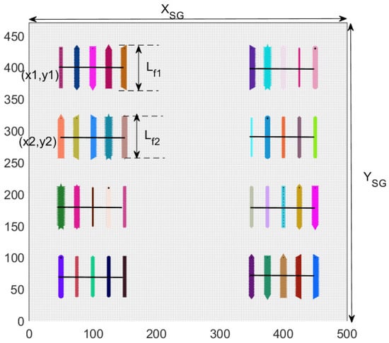
Figure 1.
Illustration of multi-well placement in shale gas reservoir. The length and width of shale gas reservoir model are and , respectively.
The integrated optimization of well placement and hydraulic fracture parameters usually run many high-fidelity model simulations. Details about the numerical equation for a unconventional shale gas reservoir model can be referred to [28]. To simplify the notation, an explicit formula of time-series shale gas production as a function of hydraulic fracture properties and well placement parameters, e.g., , is directly given here. The relationship between simulated data , e.g., time-series gas rate for producers, and the optimization variables can be described using a nonlinear operator as follows.
where, g is the nonlinear shale gas reservoir model, which represents the functions between hydraulic fractures and shale gas rate. = . The simulated data is the shale gas rate at the production timestep n. is the shale gas model simulation steps.
The integrated optimization of hydraulic fracture parameters and well placement is to determine the optimal fracture parameters and position of horizontal wells. Therefore, the multi-objectives are set as the net present value (NPV) and cumulative gas production (CPG), which can be defined as follows:
where, b is the discount rate; is the shale gas price; and represents hydraulic fracturing cost per fracture length unit.
The optimization of NPV and CPG values generally needs to satisfy some constraints, e.g., physics-laws and variables bounds. The generic formula of constrained optimization problem can be presented as follows:
where, and denote the lower and upper constraints of hydraulic parameters, including fracture number and fracture half-length and fracture spacing. In addition, the geometry of fractures should satisfy the condition that the well and fractures are located inside the reservoir domain.
The integrated optimization of fracture parameters and well placement is one of the most important engineering techniques to enhance shale gas recovery in unconventional oil and gas industry. Many mathematical optimization algorithms can be used to maximize NPV values, e.g., see Equation (4). Among them, derivative-free and derivative/gradient-based optimizations are two of the most popular categories. The key step of gradient-based optimization algorithm is to determine the gradient of the objective function with respect to the well controls. Both numerical method (deterministic gradient, e.g., finite different, or stochastic gradient, e.g., EnOpt [29] and StoSAG [30,31]) and analytical adjoint method can be used to compute the gradient. By the contrast, derivative-free methods fully regard simulators as black box with some advanced evolutionary optimizations, e.g., genetic algorithm, particle swarm optimization and differential evolution.
Due to the complex hydraulic fracture geometry [32,33] and shale gas seepage mechanisms, e.g., gas adsorption/desorption and non-Darcy flow [34,35], the computational cost of shale has reservoir model simulations is severely intensive [36,37,38]. Supported by surrogate model, these evolutionary optimizations can be very useful to resolve the high-dimensional optimizations. In this study, we employ a hierarchical surrogate-assisted evolutionary algorithm for integrated optimization of well placement and hydraulic fracture parameters in naturally fractured shale gas reservoir. In the following parts, we will give detailed descriptions about how to effectively obtain this efficient algorithm implementation in the Section 3.
3. Methods
In the section, we present an efficient global optimization framework using a novel hierarchical surrogate-assisted evolutionary algorithm and multi-fidelity modeling. The hierarchical surrogate-assisted evolutionary algorithm employs a novel multi-fidelity particle-swarm optimization of global-local hybridization searching strategy. The details related to the surrogate model and hierarchical surrogate-assisted evolutionary algorithm will be given in the following parts. In this section, the multi-layer perceptron (MLP) as a classic machine-learning-based surrogate model is used to emulate shale gas prediction models.
3.1. Definition of Multi-Layer Perceptron
At present, there are many varieties of neural networks, such as Back Propagation (BP) neural networks [39], convolutional neural networks (CNN for image recognition) [40], and long short term memory networks (LSTM for speech recognition) [41]. Multilayer perceptron is popularized from perceptron. Its main feature is that it has multiple neuron layers, so it is also called Deep Neural Networks. The combination of multilayers is an important feature of multilayer perceptron. The first, second and third layers are regarded as the input layer, middle layer and the output layer, respectively. The number of hidden layers and neurons are two of the most important hyper-parameters needed to be optimized. The optimal selection of these parameters should be optimized based on the application-specific purpose. The mathematical relationship between input and output can be presented as follows:
where, and represent the vectors of weighting coefficients and biases terms at the n-th neural network layer. denotes the activation function. The use of activation functions, including , , and (e.g., see Figure 2), is to assign the degree of non-linearity for the MLP model. The mathematical formula of activation functions can be presented as follows:
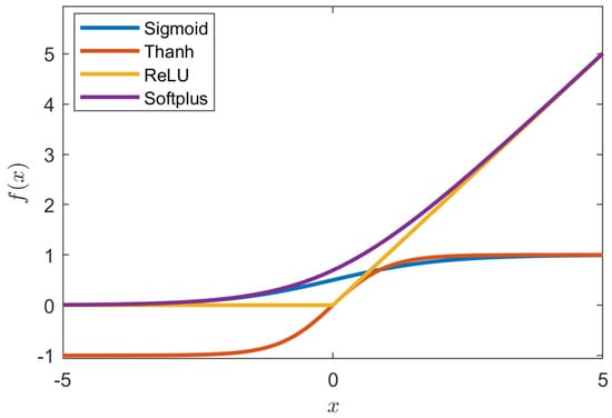
Figure 2.
Illustration of different types of activation functions, including include , , and .
In the network structure, the number of neurons in the input and output layer is determined by the given problem. Therefore, the MLP structure design only needs to consider how many hidden layers are in total, and how many neurons are in each hidden layer. Figure 3 illustrates two types of a single layer neural network model. The upper and lower subfigures denote the single output and multiple outputs, respectively. The choose of the MLP structure depends on the target.
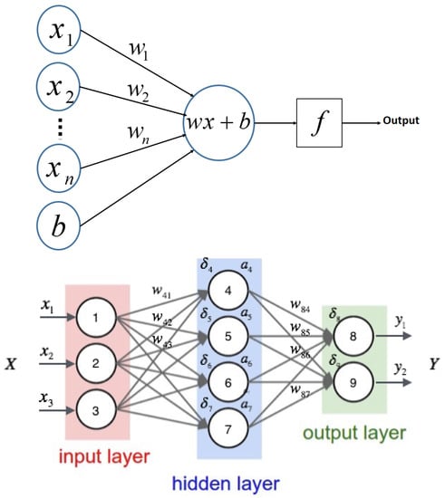
Figure 3.
Illustration of a single layer neural network model. The upper and lower subfigures denote the single output and multiple outputs, respectively.
After designing the neural network structure, we should minimize the loss function. The loss function for training the MLP surrogate model should be carefully selected to obtain good performance of the neural network model. In this paper, the desired outputs are continuous variables, e.g., time-series shale gas rate, as a result, we employ the mean square error function to cope with this vector-to-vector regression task. The loss function can be defined as
The stochastic-gradient optimizer, i.e., , is employed to optimize the neural network parameters and simultaneously [42]. In addition, some hyper-parameters, e.g., number of neurons, initial learning rate, stopping tolerance and activation function, are optimized by use of grid-search method. The quality of trained MLP surrogate model can be quantified on the testing samples. The whole process related to the model training, hyper-parameter optimization and accuracy assessment can be summarized as Figure 4. It should be noted that the running time of the new predictions through a neural network proxy model generally can be ignored in comparison with high-fidelity model simulations, which demonstrate the computational advantages of the MLP surrogate model. The quantifiable assessments related to computational cost can be referred to in the following section of numerical results. In this study, the entire process, including MLP structure design and neural network parameter training, is performed in the Matlab Deep-learning module.
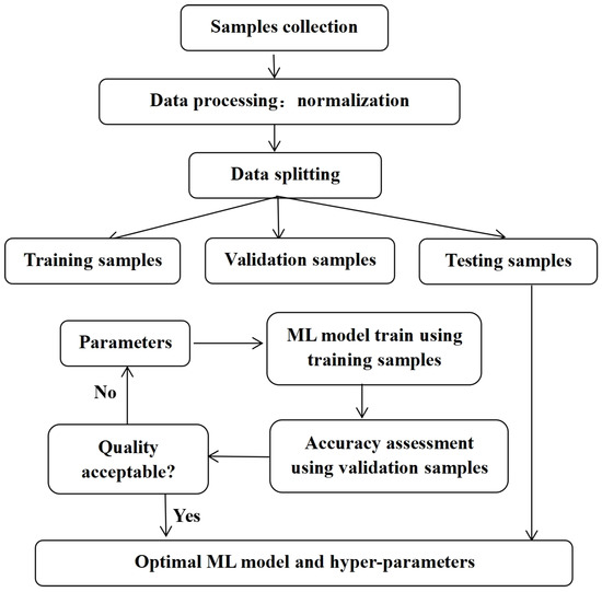
Figure 4.
Illustration of whole process related to the model training, hyper-parameter optimization and accuracy assessment.
3.2. Hierarchical Surrogate-Assisted Multi-Objective Optimization Algorithm
In the study, we propose a hybrid application of a surrogate model and particle swarm optimization for accelerating the integrated optimization of well placement and hydraulic fracture parameters in shale gas reservoirs.
The combination of the surrogate models and particle swarm optimization algorithm contributes to retain the global optimization ability of the particle swarm optimization algorithm with the help of a local surrogate model. In this paper, we use a MLP surrogate model to learn the shale gas reservoir model. Surrogate-assisted hierarchical particle swarm optimization algorithm (referred to as HS-PSO) has been extensively investigated in various fields [23]. In this paper, the algorithm is initially applied to address the integrated multi-objective optimization framework of well placement and hydraulic fracture parameters in naturally fractured shale gas reservoirs. In terms of multi-objective optimization, the non-dominated sorting genetic algorithm-II (NSGA-II) is employed to solve the defined multiobjective optimization problem. The implementation of NSGA-II algorithm can be referred to [43].
The NSGA-II algorithm is based on the particle-swarm optimization (PSO). The PSO will be simply described in this section. The evolutionary optimizations generally consist of genetic algorithm, particle swarm optimization and differential evolution. In this study, the PSO is used as the optimizer. PSO method is a kind of evolutionary computing technology, which originates from the research on the predation behavior of birds. As for the PSO algorithm, PSO is initialized as a group of random particles (random solution). For the first step, the velocity of each particle can be updated as follows:
where, 1 < i ≤ N, N is the swarm size, and are the position and velocity of the i-th particle at t-th generation, respectively. and are two random numbers. and are the i-th particle’s personal best position and global best position among the whole swarm at the current iteration. In the equation, the and are coefficients and generally set both and to 2.05, e.g., see [23].
After the velocity of each population is updated, the particle position can be presented as follows:
4. Illustrative Example and Results
In this section, several numerical experiments with varying complexity are presented to demonstrate and evaluate the performance of our proposed ML-based framework for fracture parameters and well placement optimization in the context of shale gas resources development.
4.1. Description of Model Settings
The experiment is based on a heterogeneous reservoir model with a multi-well-pad-production (e.g., see Figure 5). Two multi-stage fracturing horizontal wells are drilled in the reservoir domain. The domain size is 1200 m × 600 m. The spatial permeability fields range from 50 nD to 500 nD. In the case-study, the hydraulic fracture parameters, including fracture number and fracture half-length, and well placement (the coordinates of horizontal well toe) are regarded as the optimized variables. In all examples, MRST-Shale: an open-source shale gas simulator [44], is used to simulate the high-fidelity model (HFM) for fractured horizontal wells. This shale gas reservoir is actually modified from the real-field Barnett shale formation [44]. The basic reservoir and fluid properties, e.g., formation size, initial reservoir pressure, temperature, Langmuir coefficients, etc., are depicted in Table 1, which is referred to [44].
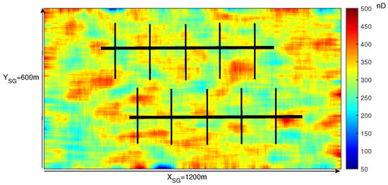
Figure 5.
Illustration of multi-well placement in shale gas reservoir. The length and width of shale gas reservoir model are and , respectively.

Table 1.
The basic reservoir and fluid properties, e.g., formation size, initial reservoir pressure, temperature, Langmuir coefficients for the shale gas reservoir model simulation using MRST-Shale [44].
4.2. Accuracy Validation of the Developed MLP Surrogate Model
To assess the quality of the trained surrogate models with respect to the training sample size, models runs are performed to generate the test samples. The quality is evaluated using the coefficients of determination () and the root means square error (), which are defined as
where and are the predictions of high-fidelity shale gas model and surrogate model, respectively. is the average values of high-fidelity model simulations. These two metrics are suitable for the assessment of regression problems.
The fracture half-length, fracture spacing, fracture number and well placement are the decision variables need to be optimized. The Figure 5 displays one realization of the parameterization of hydraulic fracture and well placement diagram of fractured horizontal well in unconventional shale reservoir. Since the NPV values depend on the shale gas production rate (e.g., see Equation (3)), the MLP surrogate model can be used to approximate the shale gas rate or NPV value directly. In this paper, since the cumulative gas rate and NPV are the bi-objectives, the surrogate model accuracy of these two strategies are investigated for the optimal selection.
The predefined correlation coefficient and root mean square error are used to quantitatively evaluate the accuracy of the machine learning model. The optimal hyperparameters are selected according to the value. The Latin-hyper-cubic (LHS) sampling method is used to randomly generate 600 datasets of decision variables, and then the high-fidelity shale gas reservoir numerical simulator is run to collect the shale gas production for 30 years, which constitutes the training datasets. Because the hydraulic fracture parameters need to be optimized, such as fracture half-length, fracture number and well placement, have different dimensions, they need to be normalized first. Overall, the 600 datasets are divided into training samples, validation samples and testing samples. The training samples are used to adjust the neural network parameters, the validation samples are used to optimize the hyperparameters, and the testing samples are used to verify the accuracy of trained MLP surrogate models.
4.2.1. Surrogate Mode for Shale Gas Rate
For the first step, we need to generate the training samples prepared for the construction of neural network model. Through running MRST-Shale simulator, these randomly generated hydraulic fracture and well placement parameters are regarded to the inputs of HFM simulations, and the simulated time-series shale gas production rates are preserved as the outputs, which constitutes the training samples.
To further improve the prediction performance of MLP surrogate model, we compress the time-series shale gas rate into low-dimension space. In this study, the principle component analysis (PCA) is used here. The decay of Eigen-spectrum of PCA is illustrated in the The first two subfigures in Figure 6a, illustrating a fast decreasing of the Eigenvalues. The evolution of relative energy with respect to the number of Eigenvalues is displayed in Figure 6b. Increasing the number of PCA patterns will preserve the dynamic features with increasingly high accuracy. For example, = 1, 5, 10 PCA patterns retain 92.3%, 99.2% and 99.8% accuracy, respectively. The last two subfigures in Figure 6c,d show the reconstructed shale gas rate and cumulative shale gas production profile. In this case-study, 10 PCA modes are almost sufficient to represent the original full-order flow dynamic.
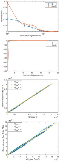
Figure 6.
The dimensionality reduction using propel component analysis. The first two subfigures show the decay of Eigen-spectrum of PCA for the shale gas rate and cumulative gas production. The last two subfigures show the crossplots of the reconstructed shale gas rate and shale gas production, respectively.
Table 2 and Table 3 show the hyperparameter optimization results. Both the and values corresponding to 100 and 500 training datasets are regarded as indicators to assess the surrogate model accuracy. In general, the higher , the better the predictability of the surrogate model. It can be seen that the prediction accuracy of machine learning models obtained from different training sets remains high, indicated by a large correlation coefficient, e.g., 95%. In this case study, the neural network model corresponding to the cumulative production of gas wells has obtained higher model accuracy, and the correlation coefficient is as high as 94%. At the same time, compared with 500 training data sets, when using 100 training data sets to build a machine learning model, the results of hyperparameter optimization show that fewer neurons (such as 32 and 128) and linear activation function can obtain the optimal model accuracy. This is because the number of neurons and the type of activation function determine the complexity of the machine learning model. More neurons and nonlinear activation functions need more training data to prevent overfitting. In this case study, when we use 500 data sets, 256 neurons and nonlinear activation functions obtain higher model accuracy.
Table 2.
The optimal grid values of hyper-parameters when using 100 training samples to train the ML models.
Table 3.
The optimal grid values of hyper-parameters when using 500 training samples to train the ML models.
Figure 7 shows the forecast results of daily and cumulative production of shale gas at three different production times (i.e., the 1st, 10th and 30th years). To verify the effect of data set size on machine-learning surrogate model, 100 and 500 data sets are used to train machine-learning models. After obtaining the trained MLP surrogate models, 100 datasets are used to test machine learning accuracy. The black line indicates the accurate prediction of the true value, and the red and blue scatter points indicate the prediction. The closer the scatter point is to the black line, the better the predictability of ML model. It can be found that the MLP model can predict all the output characteristics very well on the whole, which is very close to the black line. Compared with the cumulative gas production prediction model, the prediction of daily gas production model is relatively worse, especially when the production time is long. The RMSE predicted by the daily gas production model is much higher than that predicted by the cumulative gas production, and the score is about 0.92, which is far lower than the value predicted by the cumulative gas production. Therefore, in this case study, MLP model is more suitable for predicting cumulative gas production.
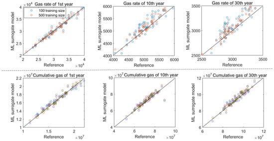
Figure 7.
Forecast results of daily production and cumulative production of shale gas at different production periods (i.e., the 1st, 10th and 30th years). The black line represents the accurate prediction of the true value, and the red and blue scatter points represent the machine learning prediction value.
To further verify the influence of dataset size on the accuracy of machine learning model, we give the relative error box diagram of the machine learning model corresponding to 100 and 500 training datasets, as shown in Figure 8. The overall average error is less than 5%, indicating a high accuracy. Compared with the daily gas production model, the relative error of the cumulative gas production prediction model is relatively small, e.g., about 2%. In addition, we also show the time series prediction of the daily gas rate and cumulative gas production of shale gas. It can be clearly revealed that the evolution trend of cumulative shale gas production can be almost correctly predicted. Increasing the number of training samples will significantly improve the prediction accuracy. We should also emphasize that even with 100 training samples, the predicted results of machine-learning surrogate model can perfectly be consist with the real results. The prediction error mainly comes from the late production time. This phenomenon can be explained as the instability of the early production stage, so it shows a high degree of nonlinearity. The production performance tends to be stable gradually, so it shows a high prediction accuracy.
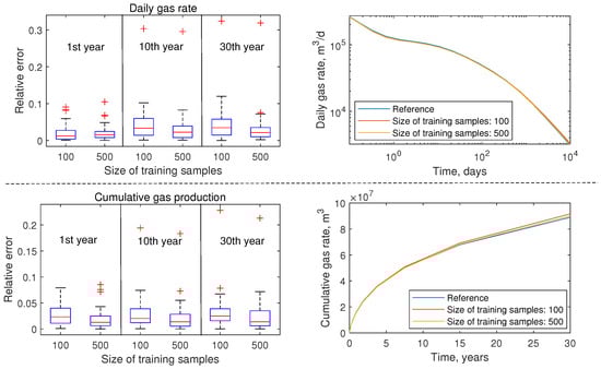
Figure 8.
Relative error box diagram of machine learning model and time series prediction results of daily and cumulative shale gas production.
It is of significance to quantify the uncertainty of shale gas production. This task is conventionally performed through running numerous shale gas reservoir simulation models parameterized by various hydraulic fracture parameters and well placement design. Based on the machine-learning surrogate model developed in this paper, we have statistically analyzed the cumulative gas production corresponding to 1000 shale gas reservoir models for 10 and 30 production years, and compared the results of conventional high-fidelity reservoir numerical simulation, as shown in Figure 9. The results show that the machine learning model and high-fidelity model obtain a consistent probability distribution, which shows a very high evaluation accuracy. In contrast, the machine learning model only needs to run 100 or 500 reservoir numerical simulations, and the calculation efficiency is extremely high.
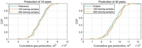
Figure 9.
Probability distribution map of cumulative gas production in 10 and 30 years of shale gas production. Machine learning model is obtained by training 100 and 500 data sets, respectively.
The proposed MLP neural network models are trained using Matlab-R2015a. The high-fidelity model simulation for the shale gas reservoir models was about 25 s; however, the proposed neural network model requires about 0.1 s. This result demonstrates a superior calculation efficiency.
4.2.2. Surrogate Mode for NPV Values
The above machine-learning surrogate models for shale gas rate demand us to train multiple MLP models for the shale gas rate at each time instance, which might increase the complexity. Since the objective of this paper is to maximize the NPV values, we can directly train MLP surrogate model for the NPV directly. Similar to the previous surrogate mode for the shale gas rate, 100 and 500 samples are used to train the surrogate models correspondingly.
Table 4 displays the hyperparameter optimization results corresponding to 100 and 500 training datasets. The different number of training samples leads to specific optimal hyperparameters. Compared to the previous surrogate model for the shale gas rate, the calculation of NPV values depends on the time-series shale gas rate and thus contains much more non-linearity. Even though only 100 training samples are used, the activation function is still required to capture the non-linearity. Figure 10 shows the evolution of loss function with respect to training epochs. It can be clearly observed that the loss functions defined on the training samples, validation samples and testing samples are gradually reduced as the iterations proceed. When training the MLP surrogate model with 100 samples, an overfitting issue has been observed, indicated by large discrepancies between training loss functions and testing loss functions. By contrast, the overfitting phenomenon does not occur with 500 training samples. It also can be clearly found that the training process of MLP surrogate model reaches the convergence rapidly, e.g., 6 and 20 epochs for the 100 and 500 training samples, respectively.
Table 4.
The optimal grid values of hyper-parameters when using 100 training samples to train the ML models.
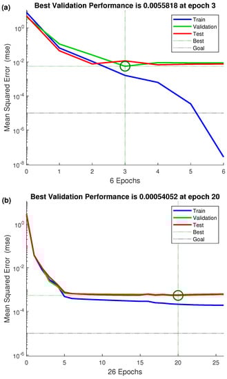
Figure 10.
The evolution of loss function with respect to epochs. The MLP surrogate models are trained by (a) 100 samples and (b) 500 samples, respectively.
Figure 11 and Figure 12 displays the crossplot results between true NPV values and surrogate-based NPV values based on the training samples, validation samples and testing samples. The predictive accuracy has been indicated by the very high correlation coefficients . In this case-study, almost all values are larger than 0.98. Solely 100 training samples can achieve very accurate results. As the number of training samples, the surrogate model accuracy improves correspondingly.
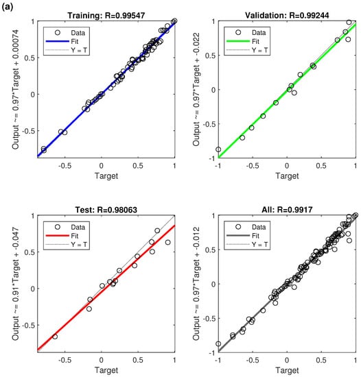
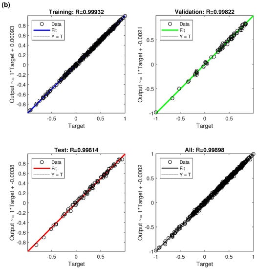
Figure 11.
The crossplot results between true values and surrogate-based values based on the training samples, validation samples and testing samples. The MLP surrogate models are trained by (a) 100 samples and (b) 500 samples, respectively.
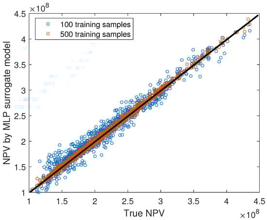
Figure 12.
The crossplot results between true values and surrogate-based values. The MLP surrogate models are trained by 100 samples and 500 samples, respectively.
4.3. Results of Integrated Optimization of Well Placement and Hydraulic Fracture Parameters
The above analysis results related to the accuracy validation of the developed MLP surrogate model reveal that the surrogate model for both shale gas rate and NPV values can obtain satisfactory accuracy. The implementation of the surrogate model for NPV values is relatively simple. In the integrated optimization of well placement and hydraulic fracture parameters, two MLP surrogate models are trained to predict the cumulative gas production and NPV values. The optimal hyper-parameters have been given in the previous section.
In this section, the trained MLP surrogate models are used to accelerate the optimization of hydraulic fracture parameters and well placement. The cumulative gas production () and net present value () are the optimized objectives. The economic parameters, e.g., shale gas price, discount and hydraulic fracturing investment cost, required by the calculations of bi-objective functions for hydraulic fracture parameters and well placement are listed in Table 1. In the base-case study, the parameters required by the PSO algorithm are also defined here. The population size and iteration step are defined as 100 and 50, respectively. To mitigate the effects of random generation of initial populations in the PSO algorithm, five independent simulation runs are performed. Figure 13 displays the final Pareto fronts results for the integrated optimization of well placement and hydraulic fracture parameters. In this base-case, the hydraulic fractures are assumed to uniform and thus only ten hydraulic fracturing parameters and well placement variables are optimized. The final Pareto fronts from these five optimization procedures become convergent at an consistent manner. That is, the optimized hydraulic fractures and well placement are almost identical.
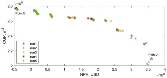
Figure 13.
Pareto fronts of 10 independent tests for one random test model.
We further choose two points from the final Pareto fronts results: the maximal NPV value (Point A) and the minimal NPV value (Point B) (Figure 13). Although the NPV values corresponding to these two points are extremely different, we can obtain almost identical fracture half-lengths, e.g., approaching to the upper bound 130 m. The differences of obtained NPV values are induced by the hydraulic fracture numbers. In this case-study, the fracture number is the controlling factors for the optimized shale gas development strategy.
The Pareto-front solutions at the final generation for all 100 (, ) realizations and the ensemble fronts (, ) obtained by the entire process of optimization workflow are shown in Figure 14a. The brown squares denote the iterative solutions, and the blue points represent the Pareto fronts. It can be clearly found that the Pareto front shows a nonlinear to some degree and the higher CGP values remained comes at the expense of lower NPV values. As can be seen from Figure 14b, the statistic distributions of optimized hydraulic fracture parameters, e.g., fracture half-length and fracture number, are gradually approaching to the parameter bounds. In this case-study, the optimized fracture half-lengths ranges from 110–130 m, while the optimized fracture numbers vary from 12 to 20. This result show that the long hydraulic fractures contribute to the shale gas production.
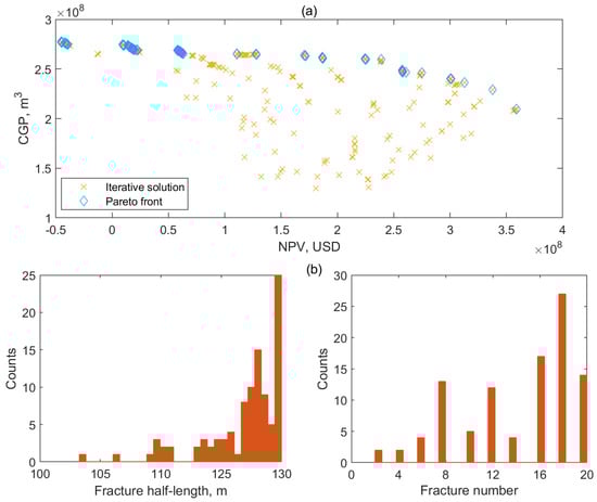
Figure 14.
Illustration of the Pareto fronts at the final generation and historical solutions (, ) over all realizations. (a) The Pareto-front solutions at the final generation and the ensemble fronts; (b) statistic distributions of optimized hydraulic fracture parameters.
In this section, we further investigate a sensitivity analysis of hyper-parameters, such as the population size and iteration steps, used in the surrogate-assisted optimization framework. Since the implementation of integrated optimization of well placement and hydraulic fracture parameters process does not involve any high-fidelity shale gas reservoir model simulations, the sensitivity analysis to the two hyper-parameters for the NSGA-II algorithm can be conducted efficiently. Figure 15 shows the Pareto fronts at the final generation for all 100 (, ) realizations with respect to different numbers of population size and iteration steps. We can also clearly find that the hyper-parameter combination of 100 population size and 100 iteration steps has almost resulted in the convergence of the NSGA-II algorithm. As has been noted earlier, since we only need to optimize two refracturing parameters, the multiobjective optimization procedure can be implemented readily. Figure 16 and Figure 17 depict the distributions of optimized hydraulic fracturing parameters with respect to different number of population size and iteration steps. All these different hyper-parameters have obtained consistent results except that 50 population size leads to slightly different results.
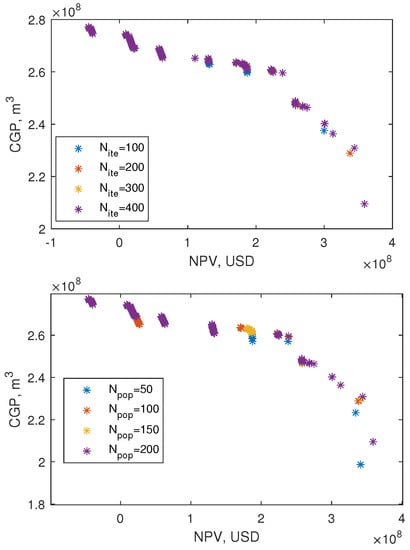
Figure 15.
Illustration of the Pareto fronts solution (, ) at the final generation with respect to population size and iteration steps for the NSGA-II algorithm.
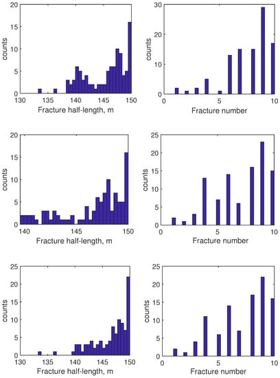
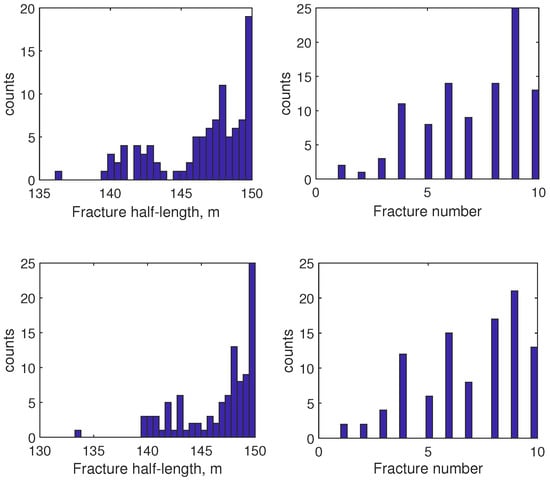
Figure 16.
Distributions of optimized hydraulic fracturing parameters with respect to the number of population sizes. The subfigures from top to the down position are corresponding to 50, 100, 150, 200 and 250 population size.
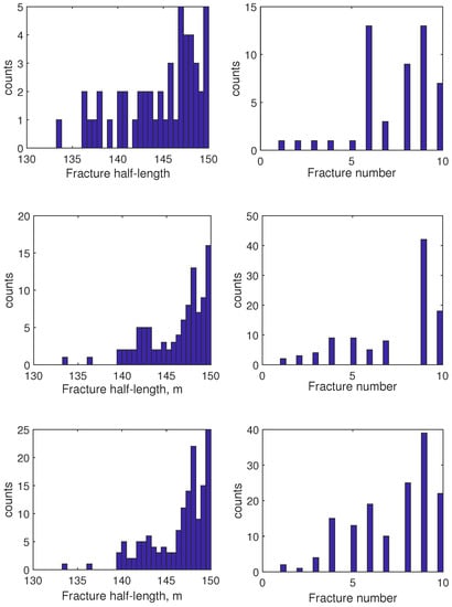
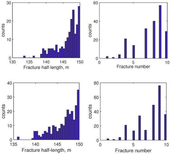
Figure 17.
Distributions of optimized hydraulic fracturing parameters with respect to the number of iteration steps. The subfigures from top to the down position are corresponding to 100, 200, 300, 400 and 500 iteration steps.
With the increasing complexity of application scenarios and the demand for prediction accuracy, the types and structures of neural networks applied to production forecasting are enriched. Deep learning models are introduced to alleviate the problem of training difficulties and gradient disappearance caused by shallow neural networks. In this study, the time-series shale gas rate is parameterized using PCA method. The PCA pattern coefficients are predicted by generic MLP surrogate model. Generally, to infer time-series production, various deep learning models such as Recurrent neural network (RNN), Convolutional neural network (CNN), Long short-term memory (LSTM), Gated recurrent unit (GRU), Bidirectional LSTM (BiLSTM) and Bidirectional GRU (BiGRU) are developed. It should be very promising to apply RNN surrogate model to emulate shale gas rate prediction. In this study, a synthetic case is used to demonstrate the accuracy and efficiency. Solely 100 training samples are sufficient to train accurate MLP surrogate model. The application of our proposed method to real-field shale gas model is very promising.
5. Conclusions
This work employs the state-of-the-art hierarchical surrogate-assisted evolutionary algorithm with the aim of accelerating integrated optimization of hydraulic fracture parameters and well placement in the community of unconventional shale gas reservoir. In terms of the accuracy and efficiency, the proposed multi-objective optimization framework is fully validated on a naturally fractured shale gas reservoir. In the integrated optimization of well placement and hydraulic fracture parameters, two MLP surrogate models are trained to predict the cumulative gas production and NPV values, respectively. The machine learning model and high-fidelity model obtain a consistent prediction results, which shows a very high evaluation accuracy. The machine learning model only needs to run 100 or 500 reservoir numerical simulations, and the calculation efficiency is extremely high. Due to the used of surrogate model, the optimization does not involve any high-fidelity shale gas reservoir simulations. The proposed framework can effectively obtain satisfactory multi-objective optimization results regarding hydraulic fracture parameters and well placement while the computational cost remains a significantly low level.
There are a few recommendations for our future work. The further applications of the proposed surrogate-based multi-objective optimization algorithm to other shale gas reservoir development problems, such as joint optimization problems and multi-objective optimization with geological uncertainty, can be investigated. Although this work restricts our focus to the particle-swarm optimizer, the surrogate-assisted evolutionary algorithm should be easily integrated with any other intelligent optimization algorithms, such as genetic algorithm, differential evolutionary, simulated annealing, etc. In addition, the decision variables that need to be optimized here are the well placements and fracture parameters, some other tasks, such as the optimization of field development plans, which includes optimizing well counts and the drilling sequence, should also benefit from our proposed optimization framework. In this study, solely the MLP surrogate mode is used. Some other proxy models, such as random forest (RF), gradient boosting (GB), extreme gradient boosting (XGBoost), light gradient boosting machine (LGBM), can also be investigated. We also can further investigates the applicability of ensemble machine learning to predict shale gas productivity. Ensemble methods with voting weight enables the individual machine learning methods complement one another and balancing the final prediction accuracy. Therefore, enhanced universality and reliability are obtained for the given learning data, permitting the successful productivity prediction of shale gas reservoirs.
Author Contributions
Conceptualization, J.Z.; methodology, J.Z.; software, J.Z.; validation, J.Z., H.W. and C.X.; formal analysis, J.Z. and H.W.; investigation, J.Z.; resources, H.W.; data curation, H.W.; writing—original draft preparation, C.X.; writing—review and editing, C.X.; visualization, C.X.; supervision, S.Z.; project administration, S.Z.; funding acquisition, S.Z. All authors have read and agreed to the published version of the manuscript.
Funding
This research was funded by Science Foundation of State Key Laboratory of Shale Oil and Gas Enrichment Mechanisms and Effective Development, grant number 35800000-22-ZC0607-0022 and The APC was funded by Science Foundation of State Key Laboratory of Shale Oil and Gas Enrichment Mechanisms and Effective Development.
Institutional Review Board Statement
The study did not require ethical approval.
Informed Consent Statement
Studies not involving humans.
Data Availability Statement
Data will be made available on request.
Acknowledgments
This work is supported by Science Foundation of State Key Laboratory of Shale Oil and Gas Enrichment Mechanisms and Effective Development (NO.35800000-22-ZC0607-0022). Computing resources are provided by Department of Petroleum Engineering at China University of Petroleum, Beijing.
Conflicts of Interest
The authors declare no conflict of interest.
Abbreviations
The following abbreviations are used in this manuscript:
| PSO | Particle swarm optimization |
| MLP | Multi-layer perceptron |
| LHS | Latin hypercube sampling |
| HS-PSO | Hierarchical Surrogate-Assisted Particle swarm optimization |
References
- Perry, S.L. Development, Land Use, and Collective Trauma: The Marcellus Shale Gas Boom in Rural Pennsylvania. Cult. Agric. 2012, 34, 81–92. [Google Scholar] [CrossRef]
- Zou, C.; Dong, D.; Wang, S.; Li, J.; Cheng, K. Geological characteristics and resource potential of shale gas in China. Pet. Explor. Dev. 2010, 37, 641–653. [Google Scholar] [CrossRef]
- Sovacool, B.K. Cornucopia or curse? Reviewing the costs and benefits of shale gas hydraulic fracturing (fracking). Renew. Sustain. Energy Rev. 2014, 37, 249–264. [Google Scholar] [CrossRef]
- Cremonese, L.; Flynn, M.P.; Gusev, A.; Lorenz, N. Shale Gas and Hydraulic Fracturing; SIWI Report 34; Stockholm International Water Institute: Stockholm, Sweden, 2014. [Google Scholar]
- Valentine, A.P.; Brown, A.; Gupta, S.; Dwivedi, P. Production Forecasting in Shales: A Comparative Field Data Study Using Large Well Counts; Society of Petroleum Engineers: Richardson, TX, USA, 2014. [Google Scholar]
- Oraon, B.; Chatterjee, A.B. Shale Reservoir Characterization & Well Productivity Analysis—Case Studies US Shale Plays (Eagle Ford and Niobrara). In Proceedings of the 11th Biennial International Conference & Exposition, Jaipur, India, 4–6 December 2015. [Google Scholar]
- Xie, J. Rapid shale gas development accelerated by the progress in key technologies: A case study of the Changning–Weiyuan National Shale Gas Demonstration Zone. Nat. Gas Ind. B 2018, 5, 283–292. [Google Scholar] [CrossRef]
- Chen, Z.; Lin, S.; Xiang, D. Mechanism of casing deformation in the Changning–Weiyuan national shale gas demonstration area and countermeasures. Nat. Gas Ind. B 2017, 4, 1–6. [Google Scholar] [CrossRef]
- Rahmanifard, H.; Plaksina, T. Application of fast analytical approach and AI optimization techniques to hydraulic fracture stage placement in shale gas reservoirs. J. Nat. Gas Sci. Eng. 2018, 52, 367–378. [Google Scholar] [CrossRef]
- Asadi, M.B.; Dejam, M.; Zendehboudi, S. Semi-analytical solution for productivity evaluation of a multi-fractured horizontal well in a bounded dual-porosity reservoir. J. Hydrol. 2020, 581, 124288. [Google Scholar] [CrossRef]
- Harb, A.; Kassem, H.; Ghorayeb, K. Black hole particle swarm optimization for well placement optimization. Comput. Geosci. 2020, 24, 1979–2000. [Google Scholar] [CrossRef]
- Wilson, K.C.; Durlofsky, L.J. Optimization of shale gas field development using direct search techniques and reduced-physics models. J. Pet. Sci. Eng. 2013, 108, 304–315. [Google Scholar] [CrossRef]
- Wang, J.; Jia, A. A general productivity model for optimization of multiple fractures with heterogeneous properties. J. Nat. Gas Sci. Eng. 2014, 21, 608–624. [Google Scholar] [CrossRef]
- Yong, R.; Chang, C.; Zhang, D.; Wu, J.; Huang, H.; Jing, D.; Zheng, J. Optimization of shale-gas horizontal well spacing based on geology–engineering–economy integration: A case study of Well Block Ning 209 in the National Shale Gas Development Demonstration Area. Nat. Gas Ind. B 2021, 8, 98–104. [Google Scholar] [CrossRef]
- Balan, H.O.; Gupta, A.; Georgi, D.T.; Al-Shawaf, A.M. Optimization of Well and Hydraulic Fracture Spacing for Tight/Shale Gas Reservoirs. In Proceedings of the SPE/AAPG/SEG Unconventional Resources Technology Conference, San Antonio, TX, USA, 1–3 August 2016. [Google Scholar]
- Yu, W.; Wang, J.; Qi, Y.; Jin, Y. Optimization of shale gas well pattern and spacing. Nat. Gas Ind. 2018, 38, 129–137. [Google Scholar]
- Rammay, M.H.; Awotunde, A.A. Stochastic optimization of hydraulic fracture and horizontal well parameters in shale gas reservoirs. J. Nat. Gas Sci. Eng. 2016, 36, 71–78. [Google Scholar] [CrossRef]
- Wang, J.; Jia, A.; Wei, Y.; Jia, C.; Yadong, Q.I.; Yuan, H.; Jin, Y. Optimization workflow for stimulation-well spacing design in a multiwell pad. Pet. Explor. Dev. 2019, 46, 1039–1050. [Google Scholar] [CrossRef]
- Xiao, C.; Zhang, S.; Ma, X.; Zhou, T.; Li, X. Surrogate-assisted hydraulic fracture optimization workflow with applications for shale gas reservoir development: A comparative study of machine learning models. Nat. Gas Ind. B 2022, 9, 219–231. [Google Scholar] [CrossRef]
- Wang, S.; Chen, S. Integrated well placement and fracture design optimization for multi-well pad development in tight oil reservoirs. Comput. Geosci. 2018, 23, 471–493. [Google Scholar] [CrossRef]
- Kumar, A.; Warren, G.; Joslin, K.; Abraham, A.; Close, J. Steam Allocation Optimization in Full Field Multi-Pad SAGD Reservoir. In Proceedings of the SPE Canada Heavy Oil Conference, Virtual, 28 September–2 October 2020. [Google Scholar]
- Pouladi, B.; Keshavarz, S.; Sharifi, M.; Ahmadi, M.A. A robust proxy for production well placement optimization problems. Fuel 2017, 206, 467–481. [Google Scholar] [CrossRef]
- Yu, H.; Tan, Y.; Zeng, J.; Sun, C.; Jin, Y. Surrogate-assisted hierarchical particle swarm optimization. Inf. Sci. 2018, 454–455, 59–72. [Google Scholar] [CrossRef]
- Cai, X.; Gao, L.; Li, X. Efficient generalized surrogate-assisted evolutionary algorithm for high-dimensional expensive problems. IEEE Trans. Evol. Comput. 2019, 24, 365–379. [Google Scholar] [CrossRef]
- Zendehboudi, S.; Rezaei, N.; Lohi, A. Applications of hybrid models in chemical, petroleum, and energy systems: A systematic review. Appl. Energy 2018, 228, 2539–2566. [Google Scholar] [CrossRef]
- Zhao, G.; Yao, Y.; Wang, L.; Adenutsi, C.D.; Feng, D.; Wu, W. Optimization design of horizontal well fracture stage placement in shale gas reservoirs based on an efficient variable-fidelity surrogate model and intelligent algorithm. Energy Rep. 2022, 8, 3589–3599. [Google Scholar] [CrossRef]
- Chen, G.; Li, Y.; Zhang, K.; Xue, X.; Yao, J. Efficient hierarchical surrogate-assisted differential evolution for high-dimensional expensive optimization. Inf. Sci. 2020, 542, 228–246. [Google Scholar] [CrossRef]
- Duong, A.N. An unconventional rate decline approach for tight and fracture-dominated gas wells. In Proceedings of the Canadian Unconventional Resources and International Petroleum Conference, Calgary, AB, Canada, 19–21 October 2010. [Google Scholar]
- Petvipusit, R. Dynamic Well Scheduling and Well Type Optimization Using Ensemble-Based Method (Enopt). Ph.D. Thesis, University of Oklahoma, Norman, OK, USA, 2011. [Google Scholar]
- Fonseca, R.R.M.; Chen, B.; Jansen, J.D.; Reynolds, A. A stochastic simplex approximate gradient (StoSAG) for optimization under uncertainty. Int. J. Numer. Methods Eng. 2017, 109, 1756–1776. [Google Scholar] [CrossRef]
- Lu, R.; Forouzanfar, F.; Reynolds, A.C. Bi-objective optimization of well placement and controls using stosag. In Proceedings of the SPE Reservoir Simulation Conference, Montgomery, TX, USA, 20–22 February 2017. [Google Scholar]
- Moinfar, A.; Varavei, A.; Sepehrnoori, K.; Johns, R.T. Development of an efficient embedded discrete fracture model for 3D compositional reservoir simulation in fractured reservoirs. SPE J. 2014, 19, 289–303. [Google Scholar] [CrossRef]
- Ţene, M.; Bosma, S.B.; Al Kobaisi, M.S.; Hajibeygi, H. Projection-based embedded discrete fracture model (pEDFM). Adv. Water Resour. 2017, 105, 205–216. [Google Scholar] [CrossRef]
- Osholake, T.; Yilin Wang, J.; Ertekin, T. Factors Affecting Hydraulically Fractured Well Performance in the Marcellus Shale Gas Reservoirs. J. Energy Resour. Technol. 2012, 135, 013402. [Google Scholar] [CrossRef]
- Meng, X.; Wang, J. Production Performance Evaluation of Multifractured Horizontal Wells in Shale Oil Reservoirs: An Analytical Method. J. Energy Resour. Technol. 2019, 141, 102907. [Google Scholar] [CrossRef]
- Ozkan, E.; Raghavan, R.S.; Apaydin, O.G. Modeling of Fluid Transfer From Shale Matrix to Fracture Network; Society of Petroleum Engineers: Richardson, TX, USA, 2010. [Google Scholar]
- Yang, R.; Huang, Z.; Yu, W.; Li, G.; Ren, W.; Zuo, L.; Tan, X.; Sepehrnoori, K.; Tian, S.; Sheng, M. A Comprehensive Model for Real Gas Transport in Shale Formations with Complex Non-planar Fracture Networks. Sci. Rep. 2016, 6, 36673. [Google Scholar] [CrossRef]
- Seales, M.B. Multiphase Flow in Highly Fractured Shale Gas Reservoirs: Review of Fundamental Concepts for Numerical Simulation. J. Energy Resour. Technol. 2020, 142, 100801. [Google Scholar] [CrossRef]
- Zhou, C.D. Applications of Back-Propagation (BP) Neural Networks and Simulated Annealing Algorithms to Log Interpretation. Well Logging Technol. 1993, 1, 30–35. [Google Scholar]
- Tajbakhsh, N.; Shin, J.Y.; Gurudu, S.R.; Hurst, R.T.; Kendall, C.B.; Gotway, M.B.; Liang, J. Convolutional Neural Networks for Medical Image Analysis: Full Training or Fine Tuning? IEEE Trans. Med. Imaging 2016, 35, 1299–1312. [Google Scholar] [CrossRef] [PubMed]
- Malhotra, P.; Vig, L.; Shroff, G.; Agarwal, P. Long Short Term Memory Networks for Anomaly Detection in Time Series. In Proceedings of the 23rd European Symposium on Artificial Neural Networks, Computational Intelligence and Machine Learning, ESANN 2015, Bruges, Belgium, 22–23 April 2015. [Google Scholar]
- Kingma, D.P.; Ba, J. Adam: A method for stochastic optimization. arXiv 2014, arXiv:1412.6980. [Google Scholar]
- Zhihuan, L.; Yinhong, L.; Xianzhong, D. Non-dominated sorting genetic algorithm-II for robust multi-objective optimal reactive power dispatch. IET Gener. Transm. Distrib. 2010, 4, 1000–1008. [Google Scholar] [CrossRef]
- Wang, B. MRST-shale: An open-source framework for generic numerical modeling of unconventional shale and tight gas reservoirs. Geosciences 2020, 11, 106. [Google Scholar] [CrossRef]
Disclaimer/Publisher’s Note: The statements, opinions and data contained in all publications are solely those of the individual author(s) and contributor(s) and not of MDPI and/or the editor(s). MDPI and/or the editor(s) disclaim responsibility for any injury to people or property resulting from any ideas, methods, instructions or products referred to in the content. |
© 2022 by the authors. Licensee MDPI, Basel, Switzerland. This article is an open access article distributed under the terms and conditions of the Creative Commons Attribution (CC BY) license (https://creativecommons.org/licenses/by/4.0/).