
Design and Control of Brushless DC Motor Drives for Refrigerated Cabinets


Abstract
:1. Introduction
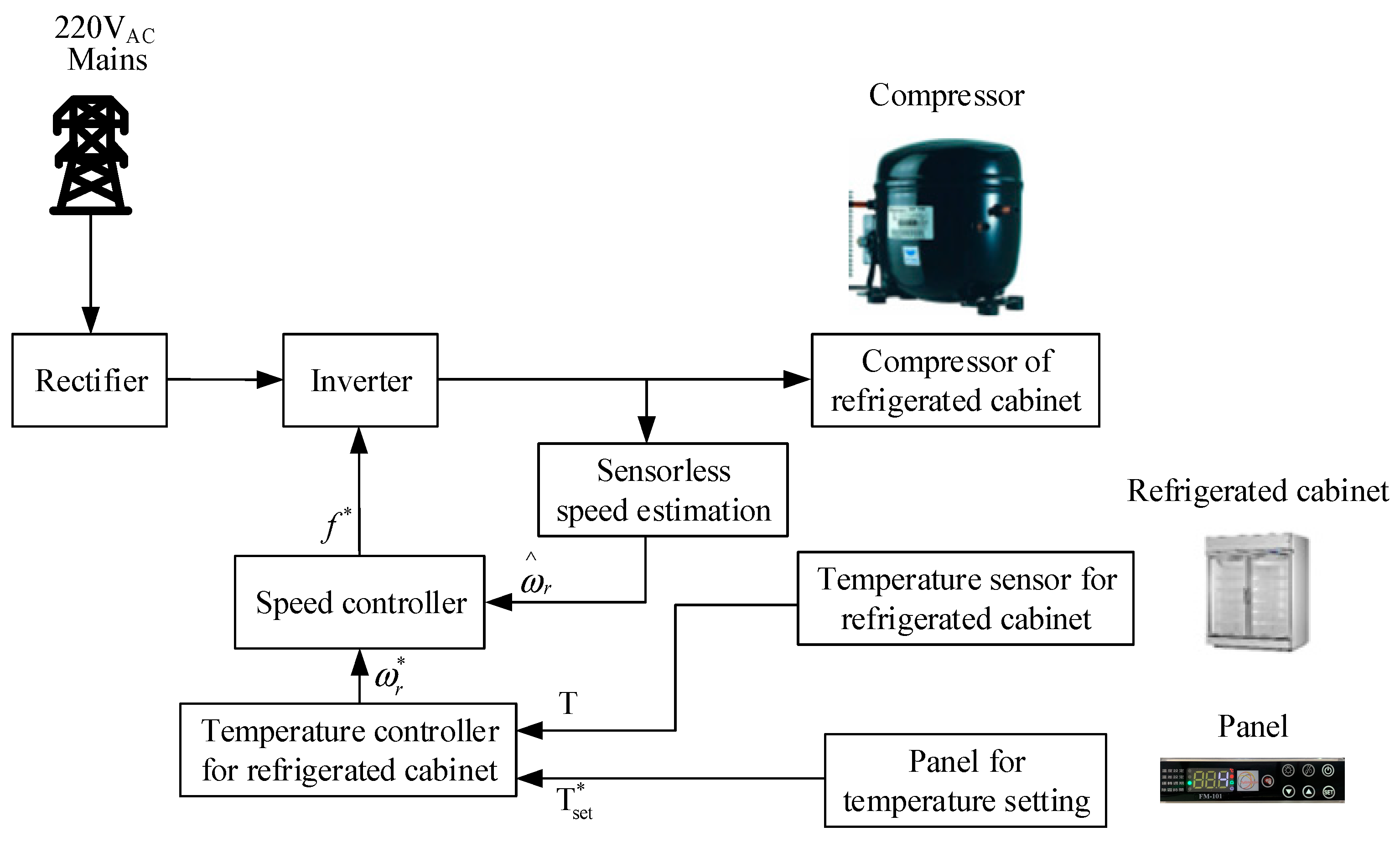
2. Architecture of Drive Control System for Refrigerated Cabinets
2.1. Design of Compressor Drives
2.1.1. EMI Suppressor
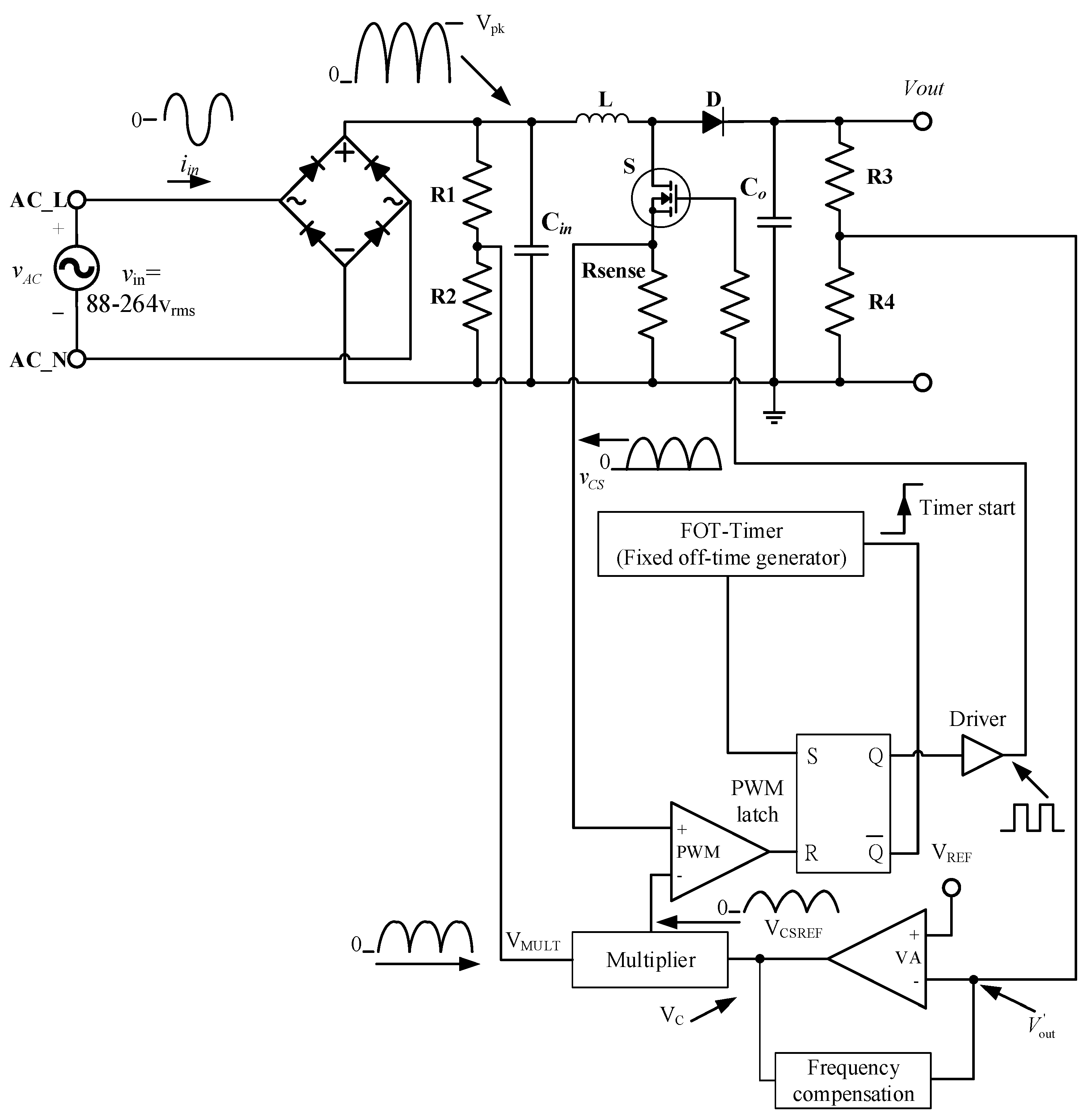
2.1.2. Power Factor Corrector
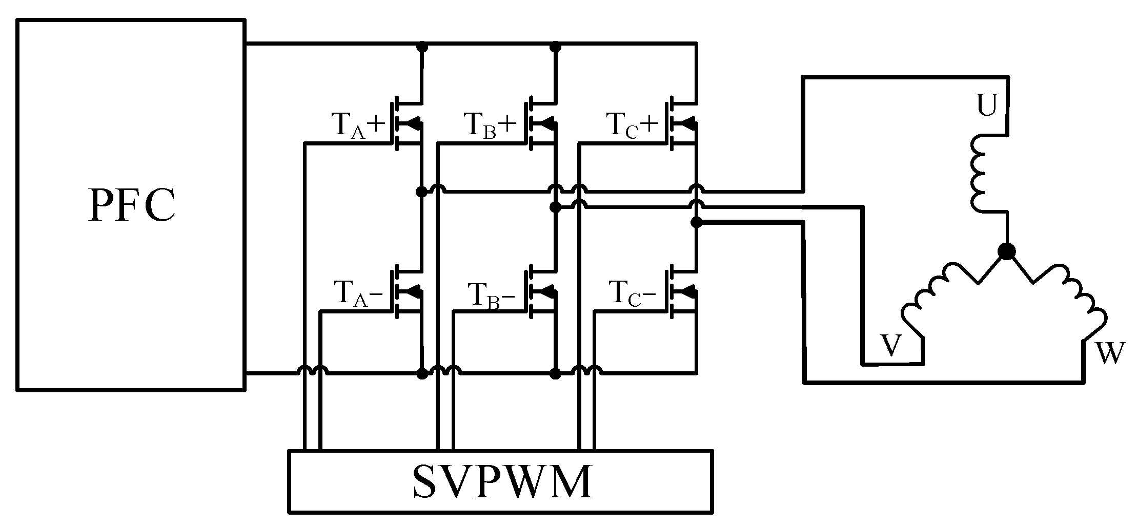
2.1.3. Space Vector Pulse Width Modulation of Inverter
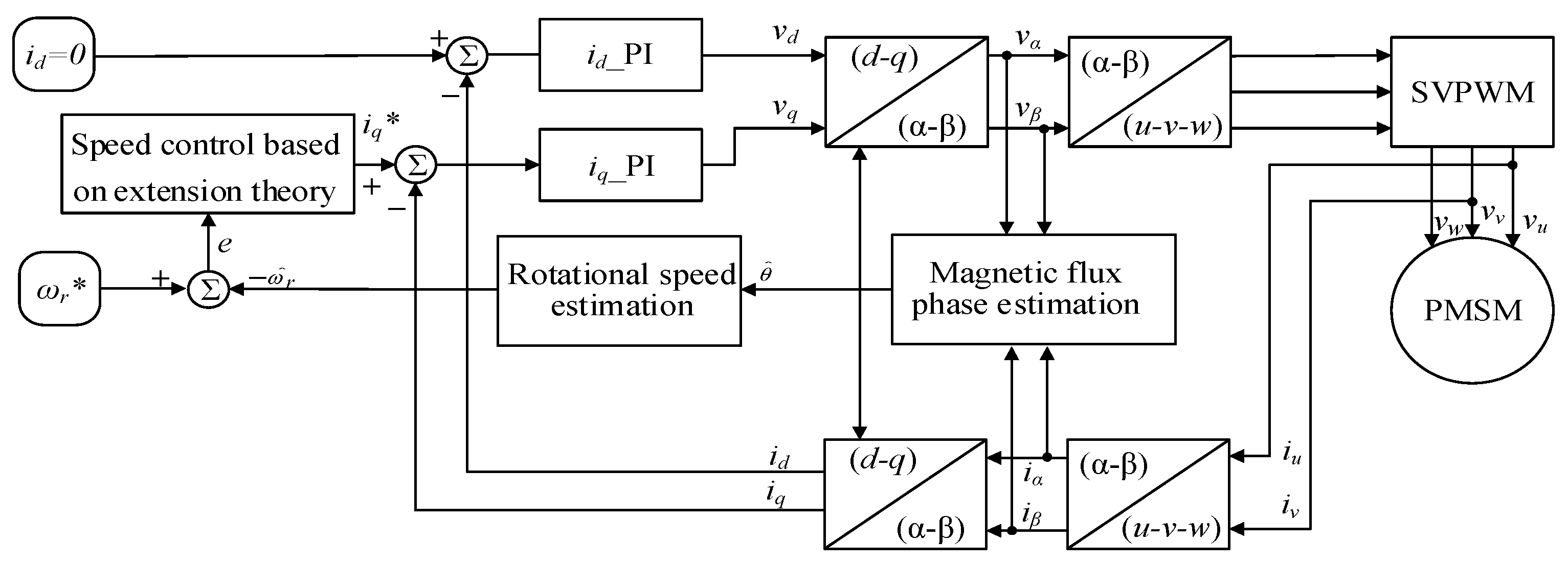
2.2. Sensorless Speed Estimation of the Inverter
3. Drive Control for the Compressor of Refrigerated Cabinet
3.1. Extension Theory
3.1.1. Extension Matter-Element Model
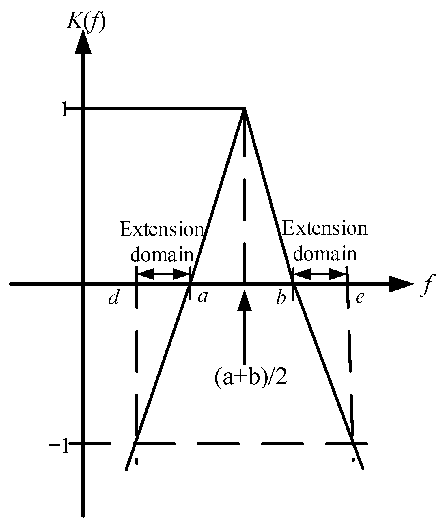
3.1.2. Definition of Classical Domain and Neighborhood Domain in Extension Theory
3.1.3. Distance and Rank Value
3.1.4. Correlation Function
3.2. Selection of the Extension Variable Frequency Control Characteristics for Refrigerated Cabinet
3.3. Rotational Speed Control by Extension Theory
- Step 1:
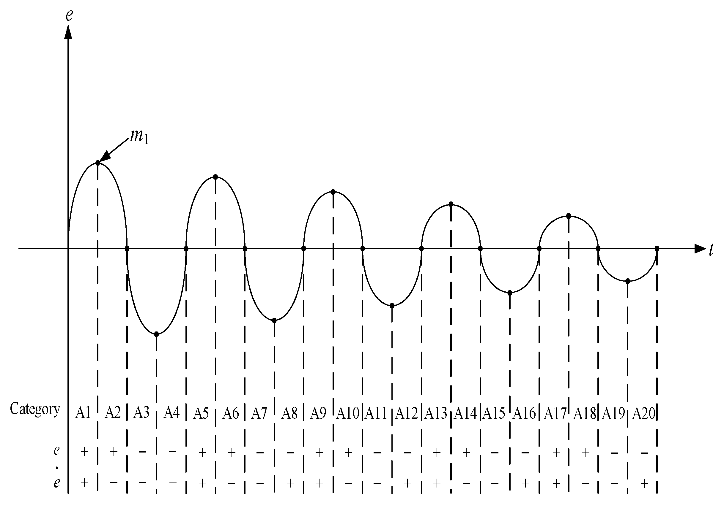
- Build the matter-element model of the characteristics for each category of the rotational speed difference and rate of change in rotational speed difference.
- Step 2:
- Input the two characteristics to be classified, the rotational speed difference and the rate of change inrotational speed difference , and the matter-element model is built as
- Step 3:
- For the rotational speed difference and the rate of change in rotational speed difference , use Equation (11) to calculate their correlation functions with each zone category.
- Step 4:
- Set the weights and for each characteristic, to represent the importance of each characteristic. For this study, both weights and are set to 1/2, and .
- Step 5:
- Calculate the correlation degree between each category’s characteristic values to be measured.
- Step 6:
- After calculation, the rotational speed difference and the rate of change in rotational speed difference to be classified will be classified into the category with the highest correlation degree and the frequency variation will be determined based on the category it belongs to. The new rotational speed frequency command is recalculated, i.e.,where is the rotational speed frequency value for the highest correlation degree calculated in the previous cycle.
- Step 7:
- The correlation degree of each classified category is normalized by using Equation (17) to have a correlation degree within the range of <−1,1>, which improves the sensitivity of the correlation degree to facilitate the classification.where and are the maximum value and minimum value of the correlation degrees for each category classified, respectively.
4. Experiment Results
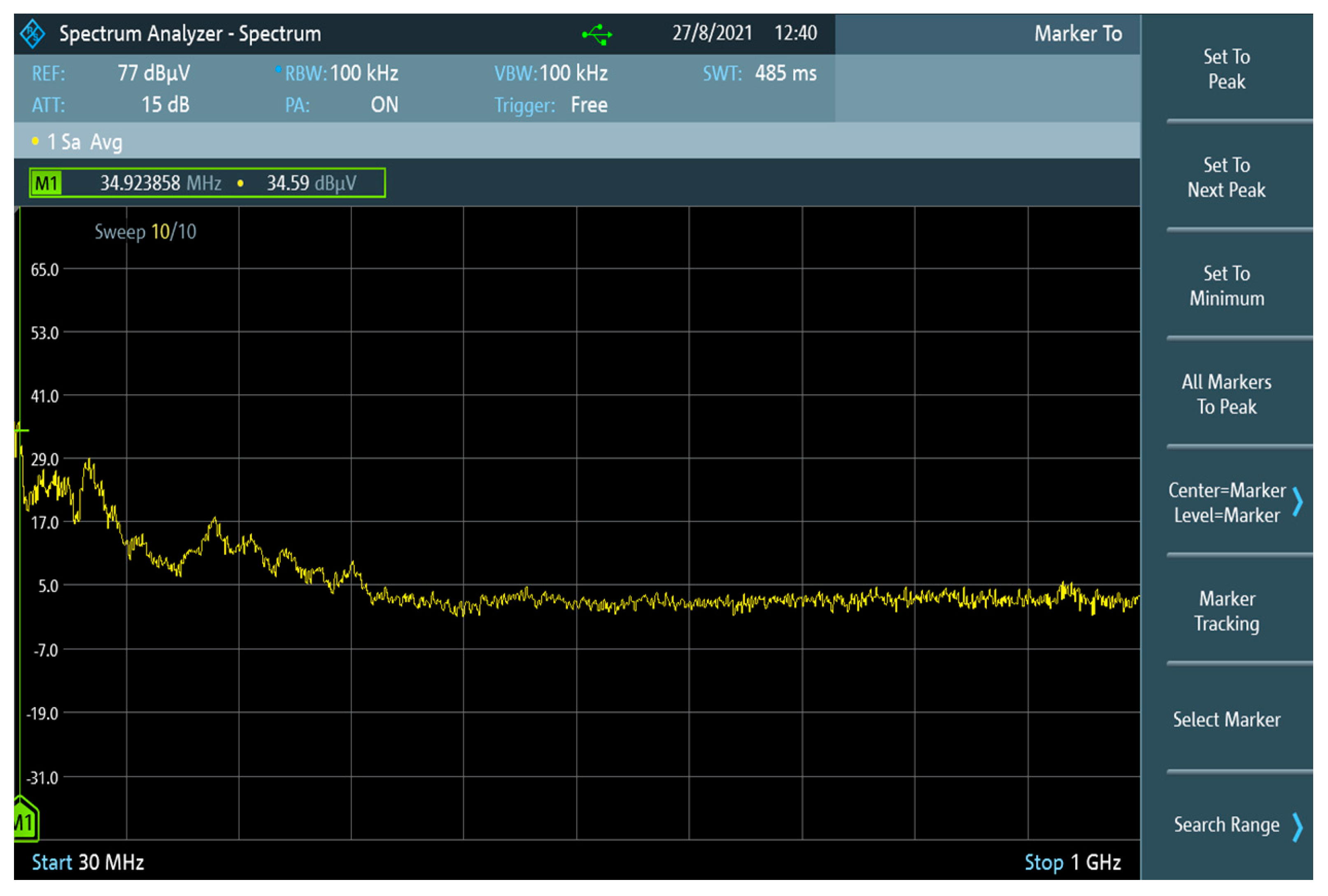
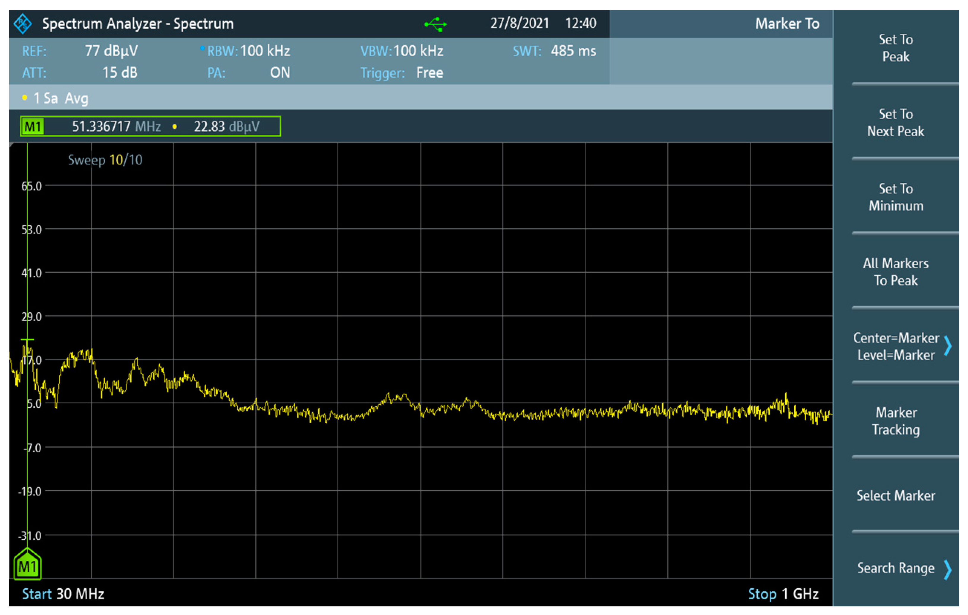
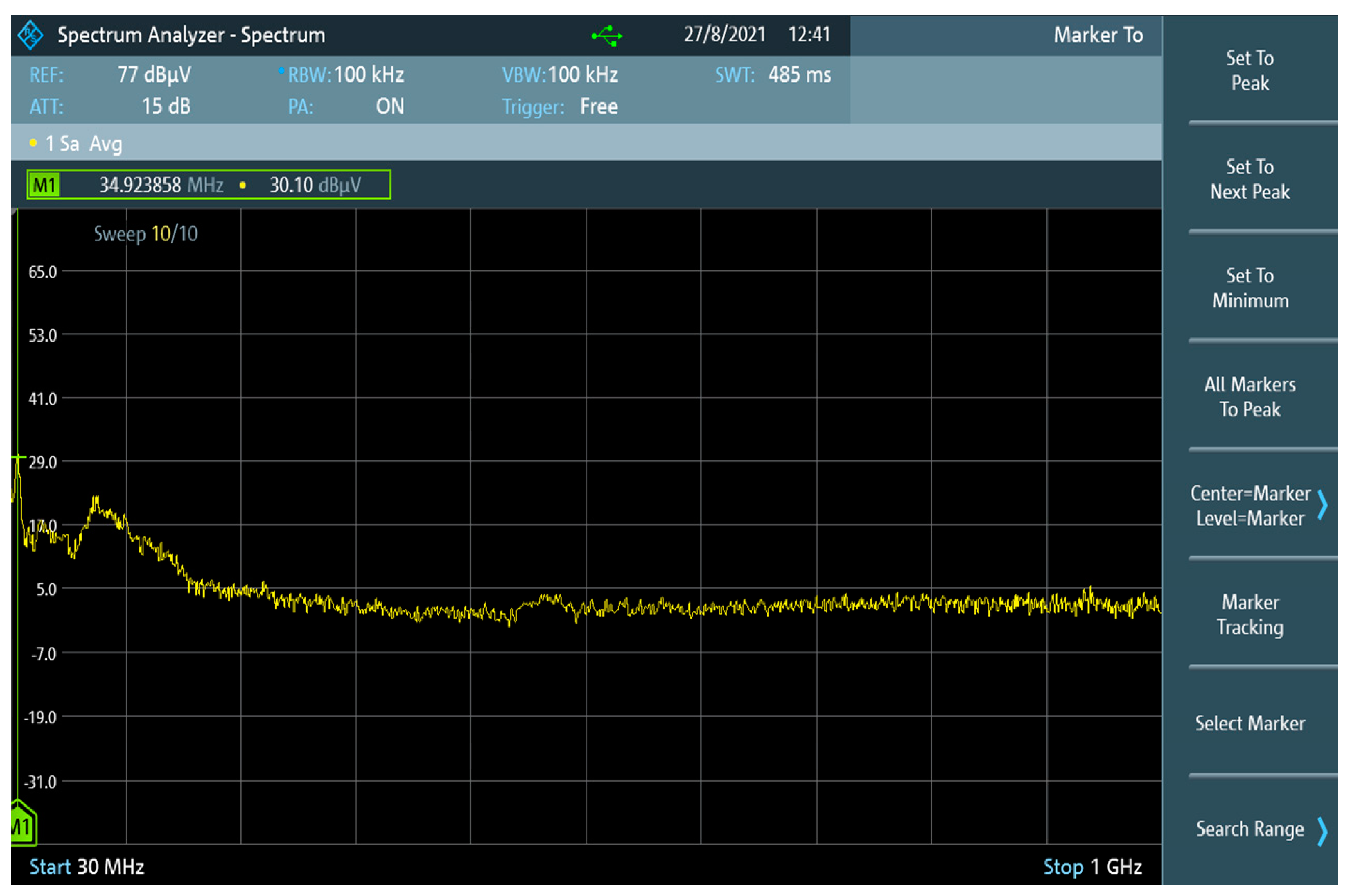
4.1. EMI Emission Suppression at the AC Input Side
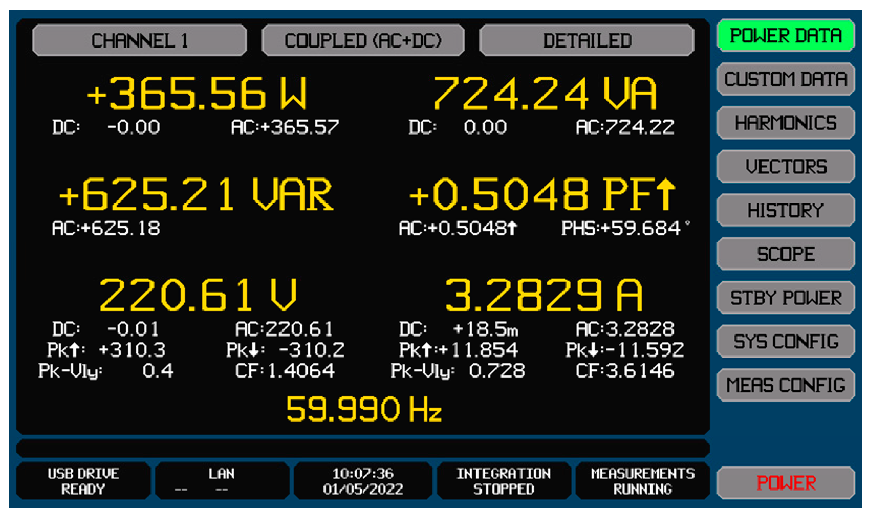
4.2. Power Quality Improvement at AC Input Side
4.3. Comparison of Power Factor and THD
4.4. Power Factor on the Output Side of the Drives
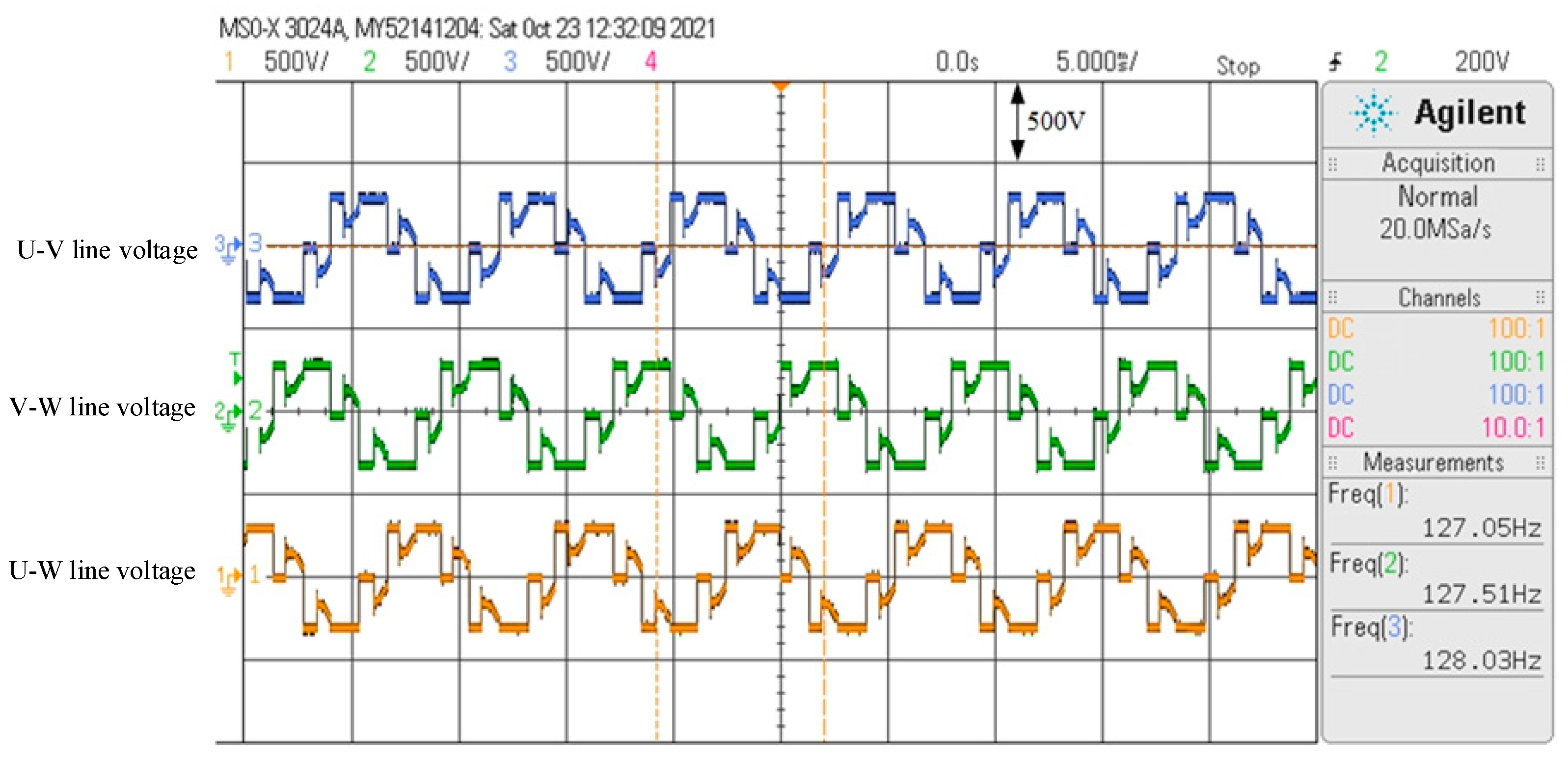
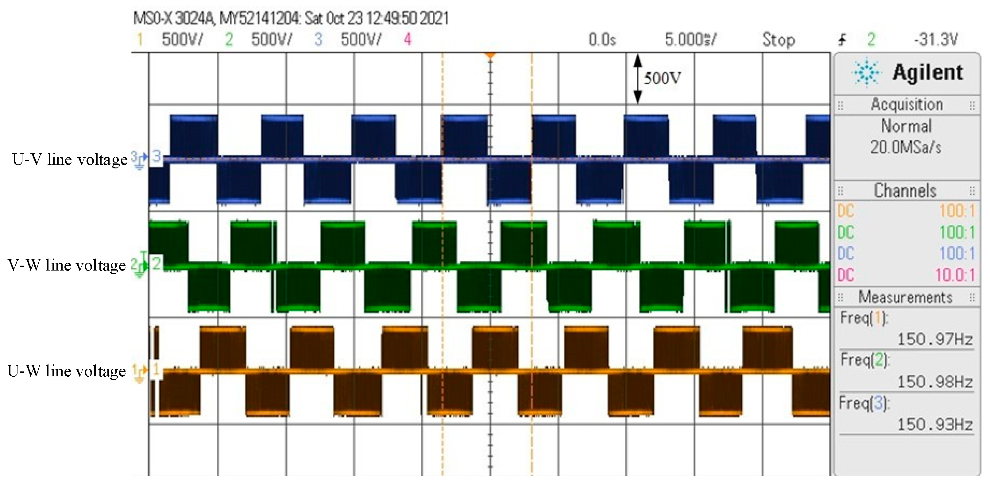
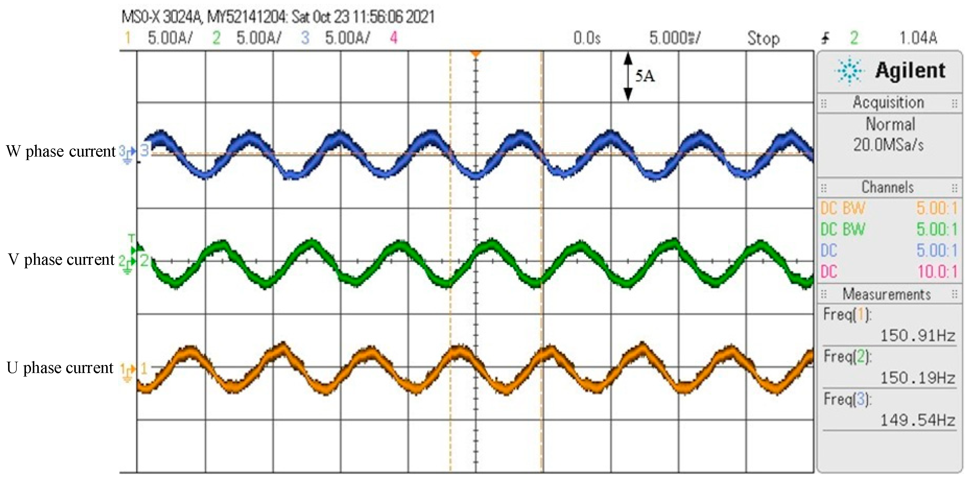
4.4.1. Comparison of the Output Line Voltage and Phase Current of the Drives
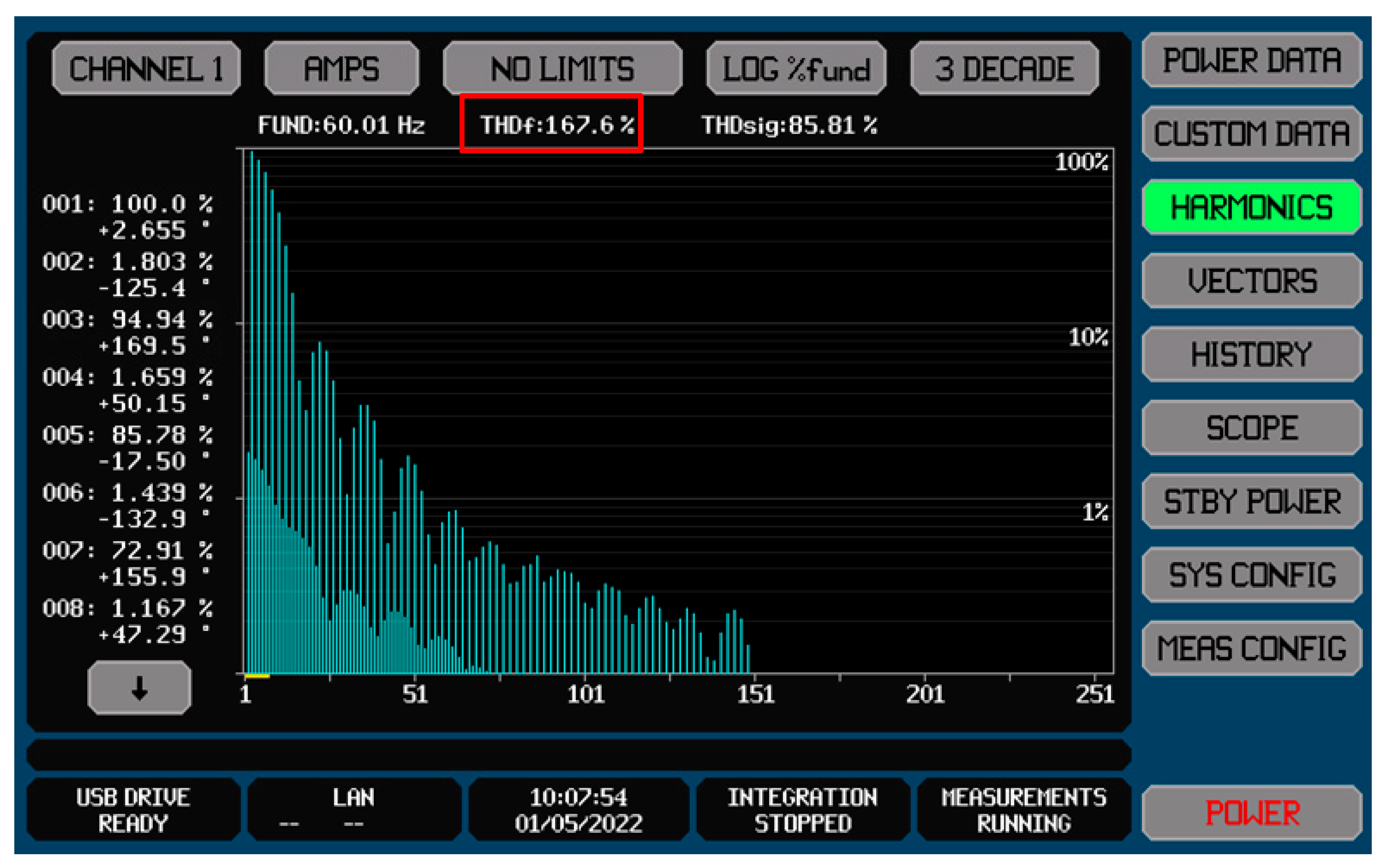
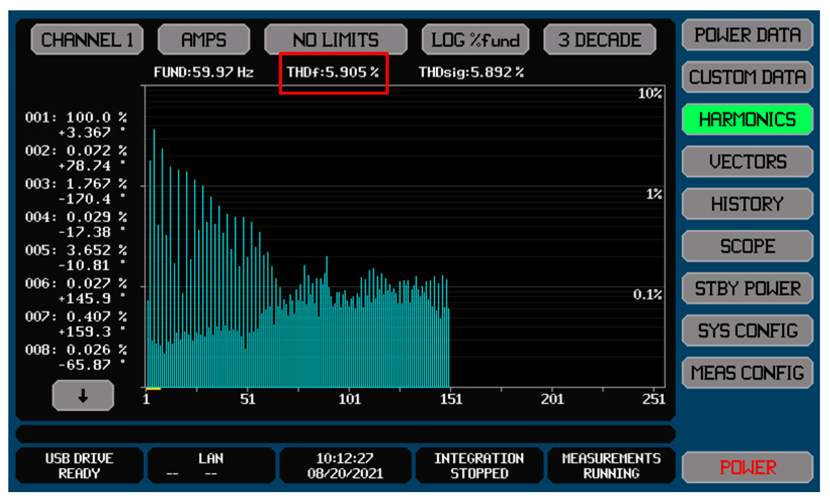
4.4.2. Comparison of the Output Current THD of the Drives
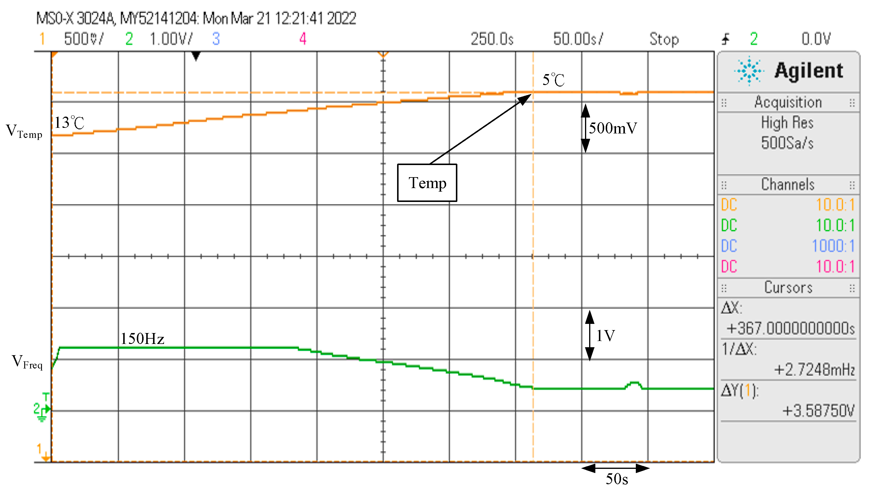
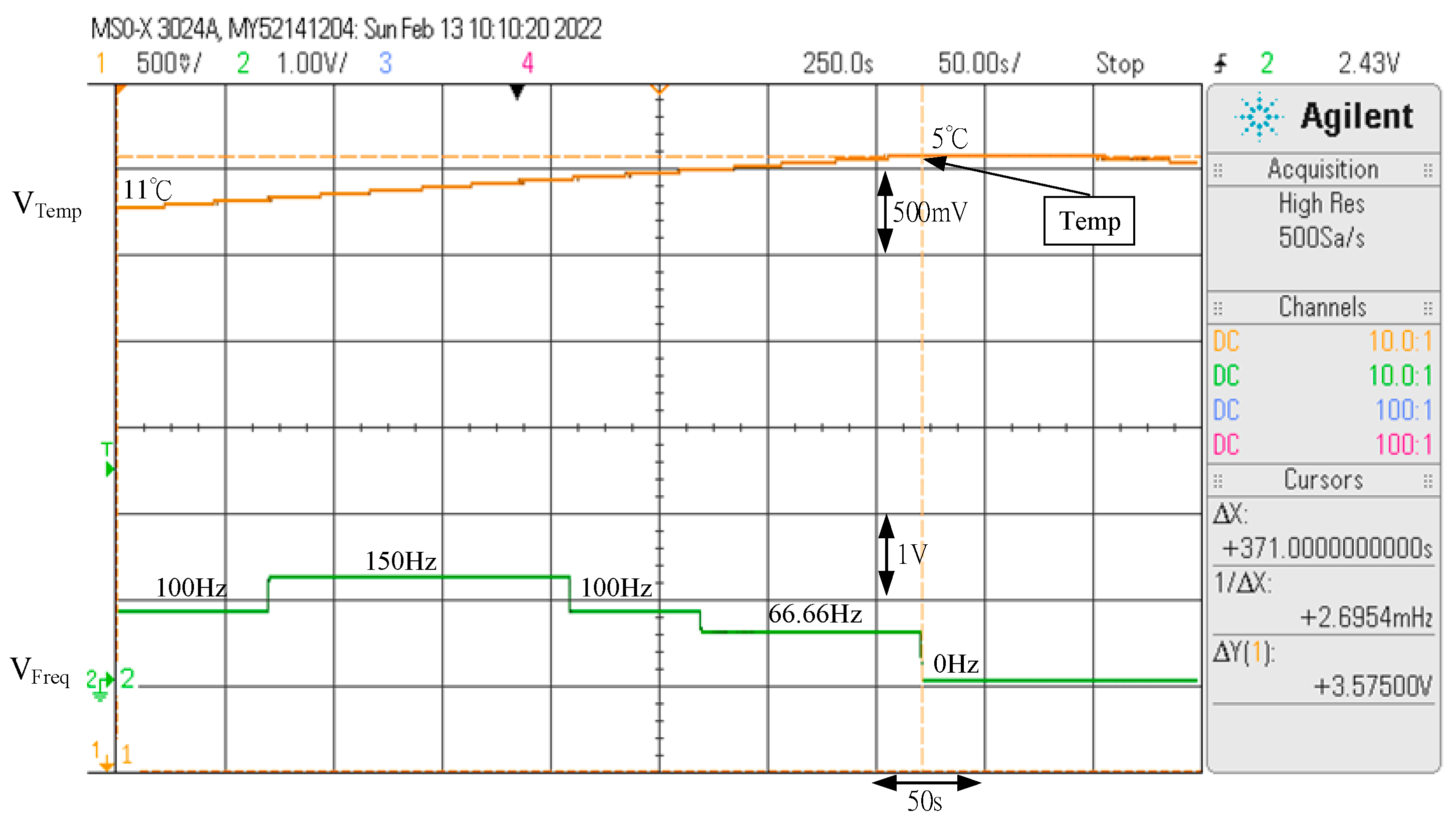
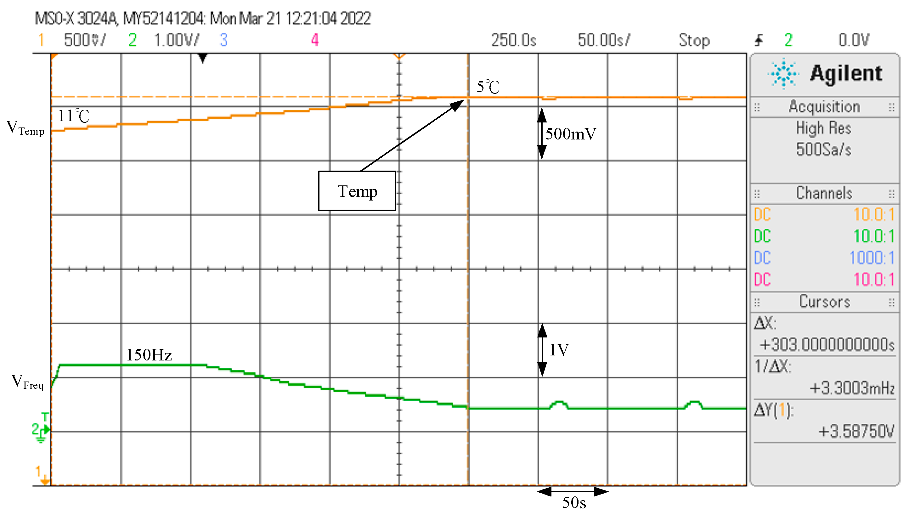
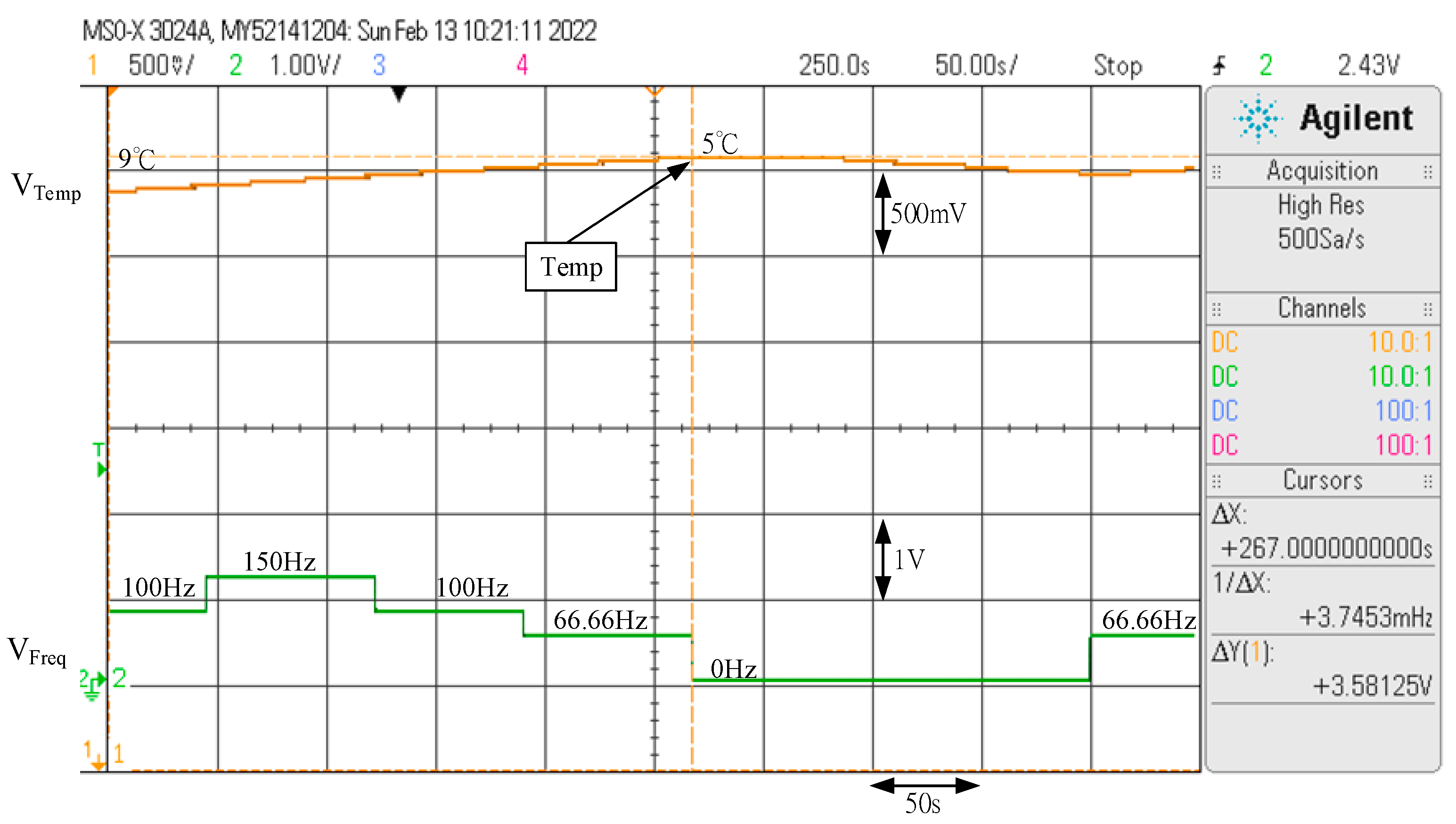
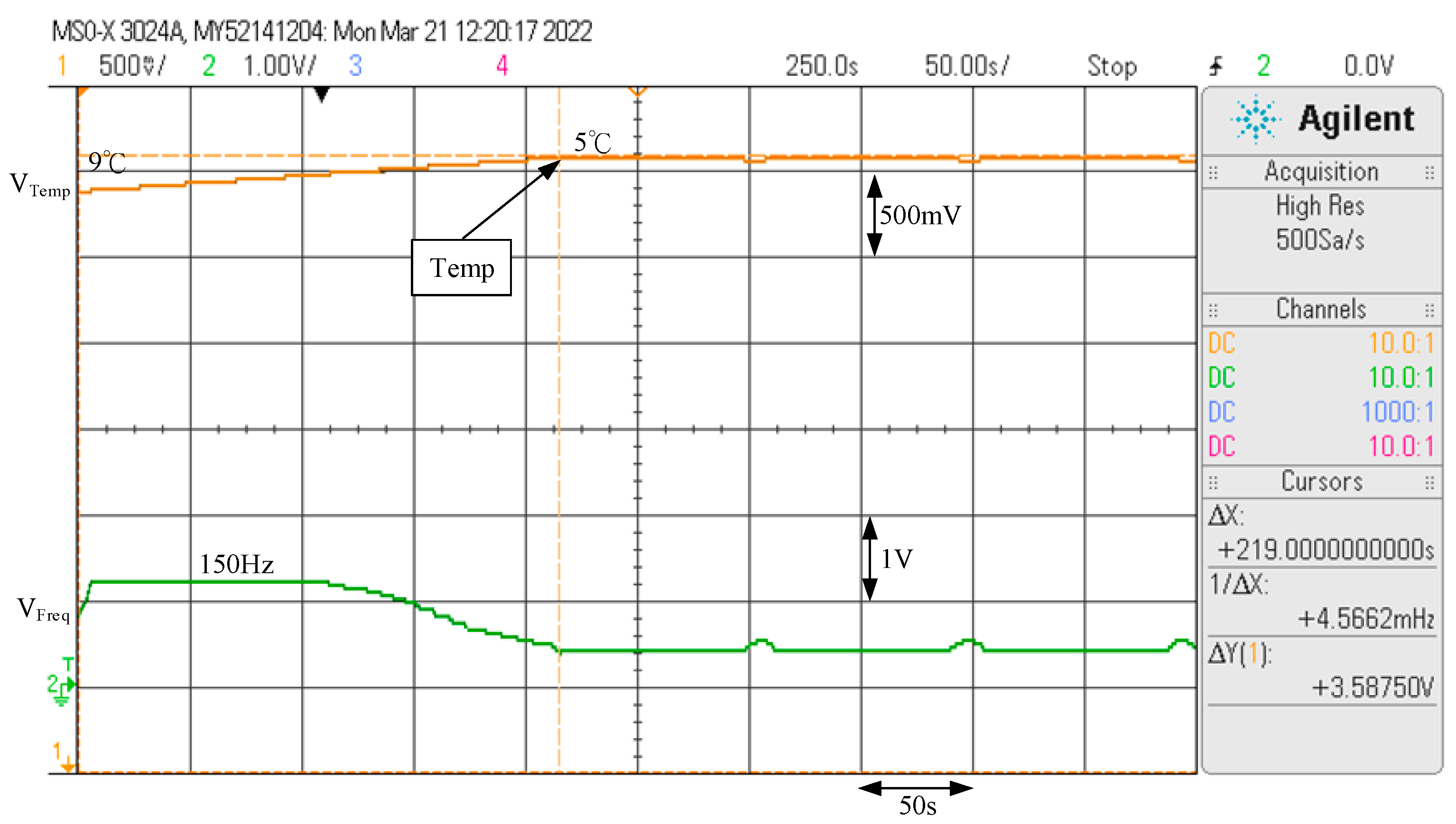
4.5. Responses of the Refrigerated Cabinet Temperature Control under Different Ambient Temperatures
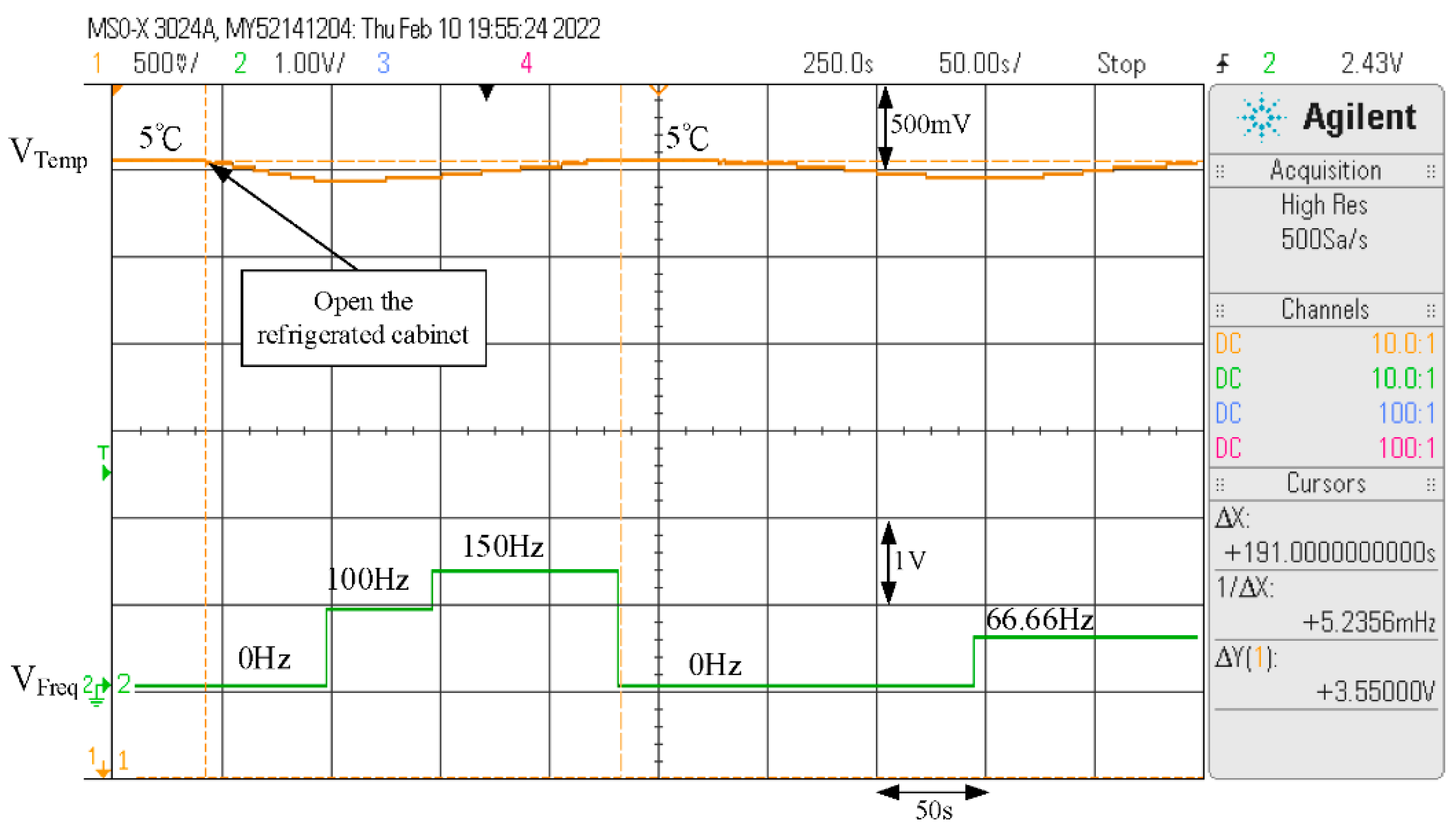
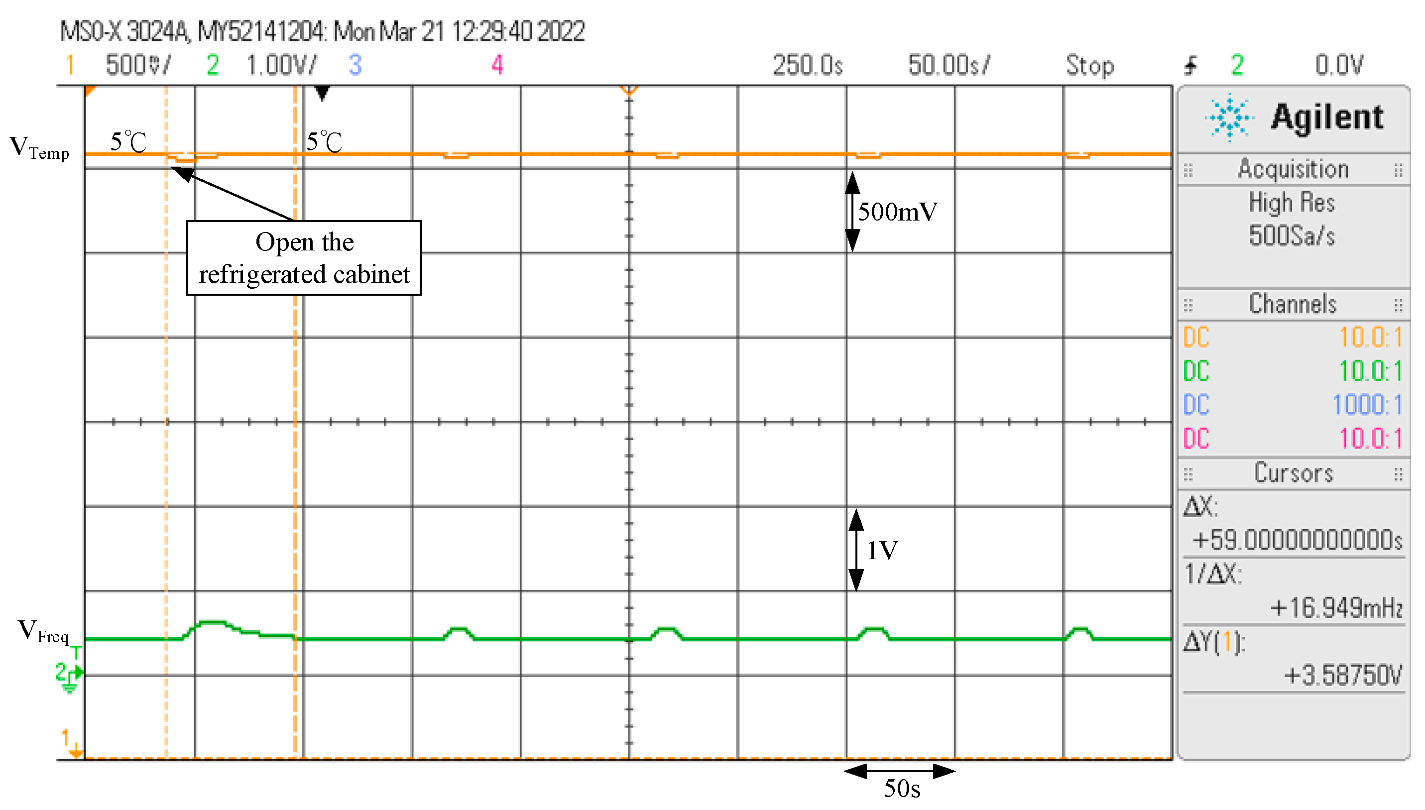
4.6. Responses of the Refrigerated Cabinet Temperature Control under the Instantaneous Change in Loads
5. Conclusions
Author Contributions
Funding
Institutional Review Board Statement
Informed Consent Statement
Data Availability Statement
Conflicts of Interest
References
- Zhang, Z.X.; Sun, B.K.; Guo, W.M.; Yuan, X.H.; Lin, T.; Liu, T. The research of an optimized three-level SVPWM strategy. In Proceedings of the 2021 IEEE 4th International Conference on Electronics Technology(ICET), Chengdu, China, 7–10 May 2021; pp. 549–553. [Google Scholar]
- Zhou, C.P.; Liu, T.; Sun, X.D.; Yang, G.J.; Su, J.Y. A dual-plane SVPWM strategy for dual three-phase PMSM. In Proceedings of the 2019 22nd International Conference on Electrical Machines and Systems (ICEMS), Harbin, China, 11–14 August 2019; pp. 1–6. [Google Scholar]
- Rachid, E.; Ahmed, A.; Muyeen, S.M. Experimental validation of a novel PI speed controller for AC motor drives with improved transient performances. IEEE Trans. Control Syst. Technol. 2018, 26, 1414–1421. [Google Scholar]
- Wang, Y.; Zhao, W.; Ai, C.; Wang, K.; Wang, H. The cooperative control of speed of underwater driving motor based on fuzzy PI control. In Proceedings of the 2020 23rd International Conference on Electrical Machines and Systems (ICEMS), Hamamatsu, Japan, 24–27 November 2020; pp. 647–651. [Google Scholar]
- Moghadasian, M.; Kianinezhad, R.; Betin, F.; Yazidi, A.; Lanfranchi, V.; Capolino, G.A. Position control of six-phase induction machine using fuzzyPI controller tuned by genetic algorithms. In Proceedings of the 2011 International Conference on Power Engineering, Energy and Electrical Drives, Malaga, Spain, 11–13 May 2011; pp. 1–6. [Google Scholar]
- Subramani, C.; Jimoh, A.A.; Kiran, S.H.; Dash, S.S. Artificial neural network based voltage stability analysis in power system. In Proceedings of the 2016 International Conference on Circuit, Power and Computing Technologies (ICCPCT), Nagercoil, India, 18–19 March 2016; pp. 1–4. [Google Scholar]
- Cheng, Y.; Li, P. Research on switched reluctance motor speed control system with variable universe fuzzy PID. In Proceedings of the 2020 IEEE 4th Information Technology, Networking, Electronic and Automation Control Conference (ITNEC), Chongqing, China, 12–14 June 2020; pp. 2285–2289. [Google Scholar]
- Cai, W. The Extension Set and Incompatibility Problem. J. Sci. Explor. 1983, 1, 81–93. [Google Scholar]
- Chen, P.Y.; Chao, K.H.; Wu, Z.Y. An Optimal Collocation Strategy for the Key Components of Compact Photovoltaic Power Generation Systems. Energies 2018, 11, 2523. [Google Scholar] [CrossRef] [Green Version]
- Chao, K.H.; Ke, C.H. Fault Diagnosis and Tolerant Control of Three-Level Neutral-Point Clamped Inverters in Motor Drives. Energies 2020, 13, 6302. [Google Scholar] [CrossRef]
- Embraco_VEGT11HB. Available online: https://www.academia.edu/40066888/_2017_catalogo_de_COMPRESSORES_HERMETICOS_EMBRACO?pop_sutd=false (accessed on 23 February 2022).
- Refrigeration Circulation System. Available online: https://www.nkhs.tp.edu.tw/resource/openfid.php?id=3546 (accessed on 10 February 2022).
- Zhang, Z.; Bazzi, A.M. Modeling, design, and implementation of a novel transformer-less feedforward-controlled active EMI filter for AC-DC power converters. In Proceedings of the 2020 IEEE Energy Conversion Congress and Exposition (ECCE), Detroit, MI, USA, 11–15 October 2016; pp. 5849–5854. [Google Scholar]
- FCC PART 15B. Available online: https://cdn-shop.adafruit.com/datasheets/SIM800_FCC_Part15.pdf (accessed on 10 February 2022).
- Mohanty, P.R.; Panda, A.K.; Das, D. An active PFC boost converter topology for power factor correction. In Proceedings of the 2015 Annual IEEE India Conference (INDICON), New Delhi, India, 17–20 December 2015; pp. 1–5. [Google Scholar]
- L4984D-CCM PFC Controller-STMicroelectronics. Available online: https://www.st.com/resource/en/datasheet/l4984d.pdf (accessed on 5 January 2022).
- Zhao, T.; Shen, W.J.; Ji, N.Y.; Liu, H.H. Study and implementation of SPWM microstepping controller for stepper motor. In Proceedings of the 2018 13th IEEE Conference on Industrial Electronics and Applications (ICIEA), Wuhan, China, 31 May–2 June 2018; pp. 2298–2302. [Google Scholar]
- Li, X.J.; Zhang, Z.L. SVPWM control of frequency-variable speed-adjustable system. In Proceedings of the 2017 IEEE International Conference on Mechatronics and Automation (ICMA), Takamatsu, Japan, 6–9 August 2017; pp. 113–118. [Google Scholar]
- Li, B.; Wang, C. Comparative analysis on PMSM control system based on SPWM and SVPWM. In Proceedings of the 2016 Chinese Control and Decision Conference (CCDC), Yinchuan, China, 28–30 August 2016; pp. 5071–5075. [Google Scholar]
- Yu, G.Q.; Zhang, Y.; Li, Y.W. Research of DSP-based SVPWM vector control system of asynchronous motor. In Proceedings of the 2012 International Conference on Computer Science and Electronics Engineering, Hangzhou, China, 23–25 March 2012; pp. 151–155. [Google Scholar]
- Yang, J.B.; Yang, G.J.; Li, T.C. Low cost sensorless vector control for PMSM compressors. In Proceedings of the 2008 International Conference on Electrical Machines and Systems, Wuhan, China, 17–20 October 2008; pp. 1456–1459. [Google Scholar]
- Renesas Electronics Corporation YROTATE-IT-RX23T. Available online: https://www.renesas.com/us/en/products/microcontrollers-microprocessors/rx-32-bit-performance-efficiency-mcus/yrotate-it-rx23t-rx23t-motor-control-reference-platform (accessed on 14 February 2022).
- Batzel, T.D.; Lee, K.Y. Electric propulsion with the sensorless permanent magnet synchronous motor: Model and approach. IEEE Trans. Energy Convers. 2005, 5, 818–825. [Google Scholar] [CrossRef]
- NTC 100K Ohm. Available online: http://www.minchuangdianzi.com/document/131.html (accessed on 24 March 2022).
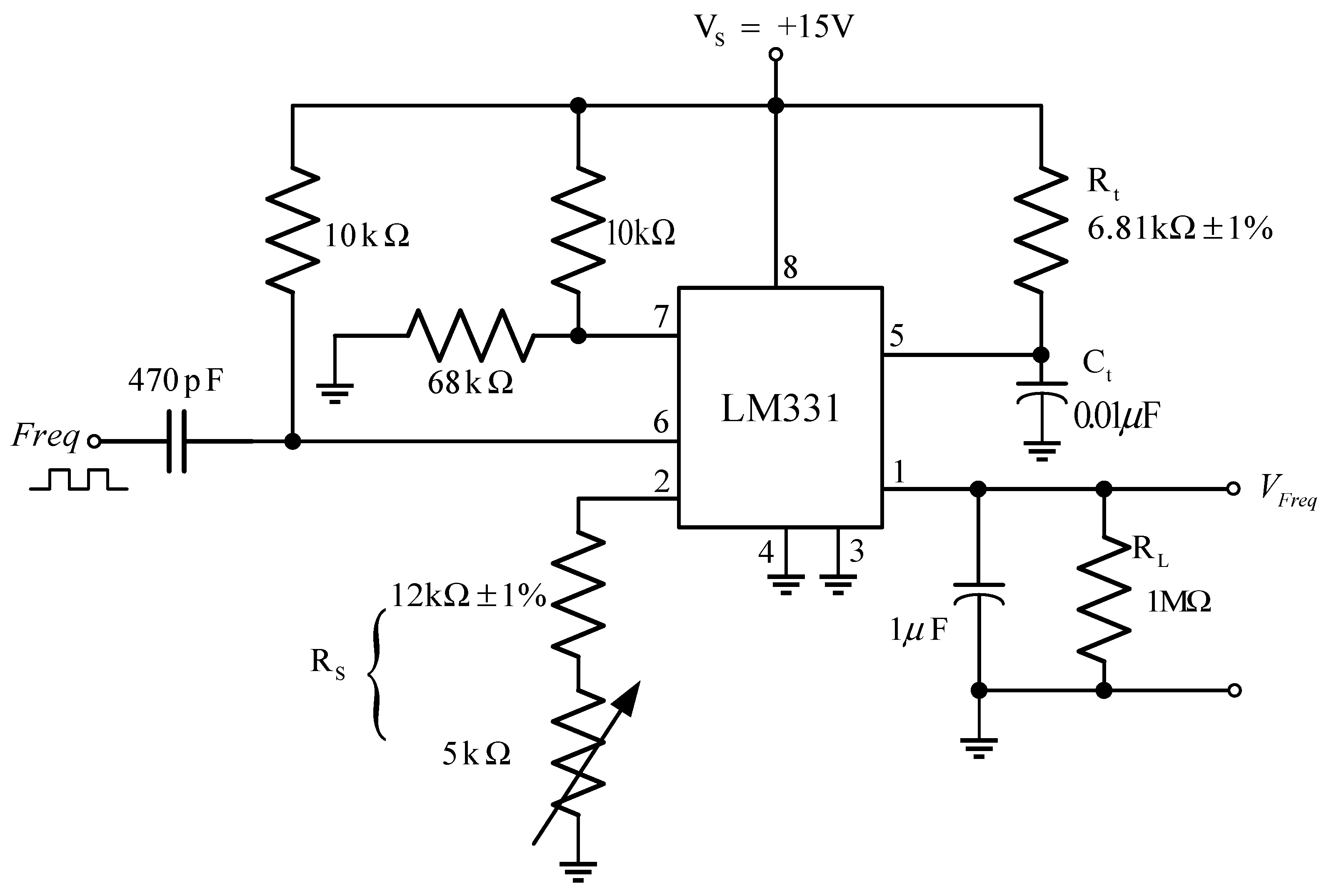
- LM331-Frequency Converter. Available online: https://www.ti.com/lit/ds/symlink/lm331.pdf?ts=1648253950571&ref_url=https%253A%252F%252Fwww.google.com%252F (accessed on 24 March 2022).


| Frequency (MHz) | Limit db (μV/m) |
|---|---|
| 30–88 | 40 |
| 88–216 | 43.5 |
| 216–960 | 46.0 |
| 960 and above | 54.0 |
| Zones | Extension Matter-Element Model | Frequency Command Variations |
|---|---|---|
| A1 | −50 | |
| A2 | −50 | |
| A3 | 50 | |
| A4 | 50 | |
| A5 | −40 | |
| A6 | −40 | |
| A7 | 40 | |
| A8 | 40 | |
| A9 | −30 | |
| A10 | −30 | |
| A11 | 30 | |
| A12 | 30 | |
| A13 | −20 | |
| A14 | −20 | |
| A15 | 20 | |
| A16 | 20 | |
| A17 | −10 | |
| A18 | −10 | |
| A19 | 10 | |
| A20 | 10 |
| Electrical Parameter | Value |
|---|---|
| Rated voltage | AC 230 V |
| Rated current | AC 3.3 A |
| Rated power | 429 W |
| Rated rotational speed | 4500 rpm |
| Input frequency range | 60–150 Hz |
| Poles | 4 |
| Electrical Parameter | Parameter Value |
|---|---|
| Input rated voltage | AC 230 V |
| Input rated current | AC 2.39 A |
| Three-phase output AC rated voltage | 240 Vrms |
| Three-phase output AC rated current | 10 A |
| Output rated power | 500 W |
| Switching frequency | 20 kHz |
| Component Name | Model/Specifications |
|---|---|
| X capacitor | 0.33 uF/300 VAC |
| Y capacitor | 1000 pF/400 V |
| Common choke | 4 mH/3.7 A |
| Rectifier | GBJ2510/25 A/1000 V |
| DC link output voltage | DC 400 V |
| DC link output current | 1.25 A |
| DC link capacitor | 450 V/680 uF |
| PFC control IC | L4984D |
| PFC power MOSFET | R6020KNX/20 A/600 V |
| PFC inductor | 1.48 mH/3.5 A |
| Intelligent power module | PSS20S92F6A-AG/20 A/600 V |
| Item | Specifications |
|---|---|
| Bit count | 32 Bits |
| Maximum Operating Frequency | 80 MHz |
| A/D converter | 12 bits |
| D/A converter | 8 bits |
| PWM control number | 4 |
| Operating voltage | 2.7 V~5.5 V |
| ROM capacity | 512 Kbytes |
| RAM capacity | 32 Kbytes |
| Flash RAM capacity | 8 Kbytes |
| Instrument Name | Manufacturer/Model | Measure Signal |
|---|---|---|
| Power analyzer | Vitrek Corporation/PA900 | Voltage, Current, Frequency, Apparent power, Real power, Power factor, Total harmonic distortion |
| Spectrum analyzer (including near field probe) | Rohde-Schwarz Ltd./FPC1000 (Rohde-Schwarz Ltd./HZ-15) | Electromagnetic interference (EMI) |
| Oscilloscope | Agilent Technologies Ltd./MSO-X 3034A | Voltage waveform, current waveform |
| Rotational Speed Command | Commercially Available Drive | Drive Developed | |||
|---|---|---|---|---|---|
| Frequency | Corresponding rotational speed | Output frequency | THDi | Output frequency | THDi |
| 150 Hz | 4500 rpm | 125 Hz | 19.96% | 150 Hz | 5.079% |
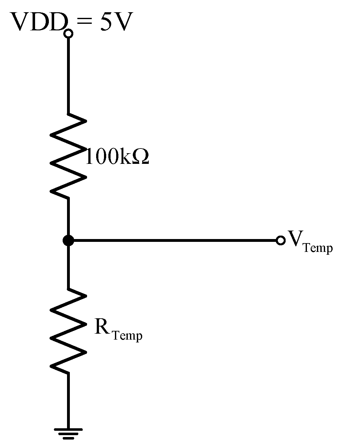
| Temp | RTemp | Temp | RTemp |
|---|---|---|---|
| 1 °C | 310.764 kΩ | 11 °C | 189.8841 kΩ |
| 2 °C | 295.4121 kΩ | 12 °C | 181.0559 kΩ |
| 3 °C | 280.9084 kΩ | 13 °C | 172.6881 kΩ |
| 4 °C | 267.2014 kΩ | 14 °C | 164.754 kΩ |
| 5 °C | 254.2428 kΩ | 15 °C | 157.229 kΩ |
| 6 °C | 241.9877 kΩ | 16 °C | 150.0898 kΩ |
| 7 °C | 230.394 kΩ | 17 °C | 143.3144 kΩ |
| 8 °C | 219.4224 kΩ | 18 °C | 136.8825 kΩ |
| 9 °C | 209.0361 kΩ | 19 °C | 130.7749 kΩ |
| 10 °C | 199.2007 kΩ | 20 °C | 124.9734 kΩ |
| Operating Condition of the Temperature Control inside the Refrigerated Cabinet | Response Time of the Conventional P-I Controller | Response Time of the Proposed Extension Controller |
|---|---|---|
| 13 °C5 °C | 434 s | 367 s |
| 11 °C5 °C | 371 s | 303 s |
| 9 °C5 °C | 267 s | 219 s |
Publisher’s Note: MDPI stays neutral with regard to jurisdictional claims in published maps and institutional affiliations. |
© 2022 by the authors. Licensee MDPI, Basel, Switzerland. This article is an open access article distributed under the terms and conditions of the Creative Commons Attribution (CC BY) license (https://creativecommons.org/licenses/by/4.0/).
Share and Cite
Chao, K.-H.; Chang, L.-Y.; Hung, C.-Y. Design and Control of Brushless DC Motor Drives for Refrigerated Cabinets. Energies 2022, 15, 3453. https://doi.org/10.3390/en15093453
Chao K-H, Chang L-Y, Hung C-Y. Design and Control of Brushless DC Motor Drives for Refrigerated Cabinets. Energies. 2022; 15(9):3453. https://doi.org/10.3390/en15093453
Chicago/Turabian StyleChao, Kuei-Hsiang, Long-Yi Chang, and Chih-Yao Hung. 2022. "Design and Control of Brushless DC Motor Drives for Refrigerated Cabinets" Energies 15, no. 9: 3453. https://doi.org/10.3390/en15093453
APA StyleChao, K.-H., Chang, L.-Y., & Hung, C.-Y. (2022). Design and Control of Brushless DC Motor Drives for Refrigerated Cabinets. Energies, 15(9), 3453. https://doi.org/10.3390/en15093453