Article

Closed-Loop Adaptive High-Starting Torque Scalar Control Scheme for Induction Motor Variable Speed Drives

by
Juan Carlos Travieso-Torres
1,*,
Manuel A. Duarte-Mermoud
2,3,
Matías Díaz
4,
Camilo Contreras-Jara
1 and
Francisco Hernández
1
1
Department of Industrial Technologies, University of Santiago de Chile, Santiago 9170125, Chile
2
Facultad de Ingeniería y Arquitectura, Universidad Central de Chile, Av. Santa Isabel 1186, Santiago 8330601, Chile
3
Advanced Mining Technology Center, University of Chile, Av. Tupper 2007, Santiago 8370451, Chile
4
Department of Electrical Engineering, University of Santiago de Chile, Santiago 9170125, Chile
*
Author to whom correspondence should be addressed.
Energies 2022, 15(10), 3489; https://doi.org/10.3390/en15103489
Submission received: 4 April 2022 / Revised: 27 April 2022 / Accepted: 29 April 2022 / Published: 10 May 2022
(This article belongs to the Special Issue Design and Control of Electrical Motor Drives II)

Abstract

:
This article proposes a closed-loop (CL) high-starting torque (HST) scalar control scheme (SCS) for induction motors (IM). It endows the recently proposed HST-SCS with high-output torque capability beyond starting after using an outer speed control loop feeding an inner current control loop with adaptive controllers. Presenting a cascade normalized adaptive passivity-based controller (N-APBC) for nonlinear systems encompassing the IM allows obtaining this result. It extends the normalized adaptive controller for the cascade case. As a result, it keeps the HST-SCS simple control scheme without needing variable observers or parameter estimators and employing tuning information only from the motor nameplate and datasheet. Test bench experiments with a 10 HP motor validate the proposal’s effectiveness. Comparative experimental results show that the CL HST-SCS has a required stator phase voltage lower than HST-SCS. The CL HST-SCS applies the adaptive starting voltage curve for a more extended time than HST-SCS, from the start to 1.9 s versus 1.2 s, respectively. Hence, CL HST-SCS assures HST not only for starting but almost up to 600 rpm, resulting in a smoother transient behavior than HST-SCS under this speed.

1. Introduction

Variable speed drive (VSD) applications [1] widely use IM [2]. This is due to its lower cost, higher efficiency, and lower maintenance compared with other electric motors.
The VSD performing the scalar control scheme (SCS) [3] mainly moves blowers, fans, and centrifugal pumps [4]. These low-performance applications demand a starting electromagnetic torque of up to 25% of the nominal torque, corresponding to the capacity of the standard SCS. Moreover, the SCS has nonrapid and even oscillatory transient speed behavior with a steady-state speed-accuracy between 1% to 4% for higher speeds [
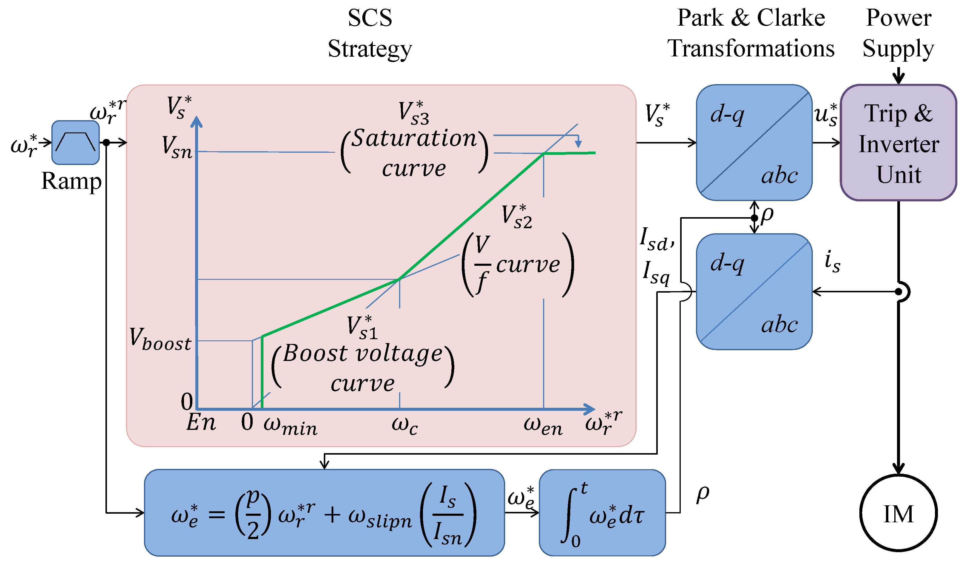
5]. Furthermore, it has the most straightforward control scheme without parameter estimates or variable observers, as shown in Figure 1.
Standard SCS follows the required rotor angular speed ω r * after establishing the necessary angular electrical frequency ω e * and stator voltage amplitude V s * . It applies a boost voltage V b o o s t , adjusted from 3% to 50% of V s n , to assure a starting electromagnetic torque from 0.09% to 25% of the rated torque. It acts at the minimum angular frequency ω m i n , tuned from 3% to 6% of the rated angular electrical frequency ω e n = 4 π f n p , to protect the IM from overcurrent consumption. Later, at the cut angular frequency ω c , tuned from 40% to 50% of ω e n , it switches to the V / f curve, which also saturates at the rated voltage for IM protection [6].
Based on previous information, the following sections describe this paper’s motivation, background, related work, and claims.

1.1. Motivation

Several researchers aim to improve the SCS scheme. Beyond studying the speed oscillations across the boost voltage curve, the work [5] proposes two methods to mitigate them. To enhance the steady-state accuracy of the actual rotor angular speed, reference [7] uses a closed-loop speed control. Moreover, reference [8] proposes a PI slip controller.
Other proposals develop a slip speed estimator based on an electromagnetic torque estimation in [9], on a gap power estimation in [10], and on a stator flux observer in [11]. Based on the ratio between the rated slip and rated stator current, references [6,12] calculate the slip. Furthermore, the work [13] proposes an optimal V/f ratio based on a reactive power estimate. These proposals require IM parameters or variable estimation, with the exception of [6].
Moreover, other works focus on improving the reduced starting electromagnetic torque SCS issue reported in [14,15]. The solution given in [14] needs stator resistance and a flux estimator. At the same time, the proposal [15] avoids parameters and variable estimators, keeping a simple control scheme. Later, reference [16] gives an alternative solution to the novel method given in [15]. It assures less stator current composition and faster speed response than the standard SCS [6], with no need for the minimum angular frequency ω m i n .
This paper aims to further improve [16] results, taking into account the following background information.

1.2. Background

The work [15] calls its solution high-starting torque (HST)-SCS. It has a multiple-input and multiple-output (MIMO) APBC that switches to the standard boost voltage curve of the SCS [6], causing curve speed and current chattering issues. The proposal [16] solves these issues after presenting a scalar output normalized APBC that smoothly switches to the standard boost voltage curve of the SCS [6]. As a result, reference [16] expands the applications of the standard SCS [6], including HST capability and keeping a simple control scheme without parameter or variable estimation. It can move, for instance, loaded conveyor belts requiring 100% of the nominal torque at the start and low steady-state speed-accuracy [16].
As an alternative to the APBC controller [16], the work [17] proposes using a normalized MRAC in the HST-SCS with good results. This paper also aims to further improve [16] by suggesting a different adaptive controller. The following section describes the details.

1.3. Related Works

All previously discussed starting adaptive control algorithms are based on the adaptive concepts given in [18] for a model reference adaptive controller (MRAC). The work [15] uses an adaptive passivity-based controller (APBC), reducing the trial and error APBC adjustment given in [19]. Nevertheless, the normalized APBC proposed in [16] further improves the APBC tuning [15] with a solution less dependent on the operational range and motor power. The work [17] proposes using a normalized MRAC, extending the direct approach described in [18].
So far, all HST-SCS, including this paper’s proposal, use a pure adaptive controller, active only during starting. Hence, these are not gain scheduling controllers such as the one used in [20] to control a brushless DC motor. This paper extends the cascade APBC proposed in [21] and applies it to the HST-SCS of IM, as the following describes.

1.4. Claims

This paper’s main contribution is proposing a CL HST-SCS based on a cascade normalized-APBC (N-APBC). It starts expanding the standard cascade APBC proposed in [21], normalizing the information vector and adaptive law gains for a more straightforward tuning method. Later, the cascade N-APBC design regulates the IM starting stator current decreasing the current consumption, diminishing IM stress and failure risk due to this cause [22]. The solution keeps the simplicity of the SCS, only using tuning information from the motor nameplate and datasheet, not needing variable observers or parameter estimators. It applies the slip speed calculation’s industry solution of [6].
This paper’s organization is as follows. The Preliminaries Section describes the basic HST-SCS, including its block diagram, control strategy, and method fundamentals. Later, Section 3 describes the proposed CL HST-SCS with the its block diagram, remarking the differences and the closed-loop control strategy. The Experimental Results Section tests both CL HST-SCS and HST-SCS strategies and describes the obtained results. Finally, the Conclusion Section presents the main findings summary.

2. Preliminaries of the Basic HST-SCS

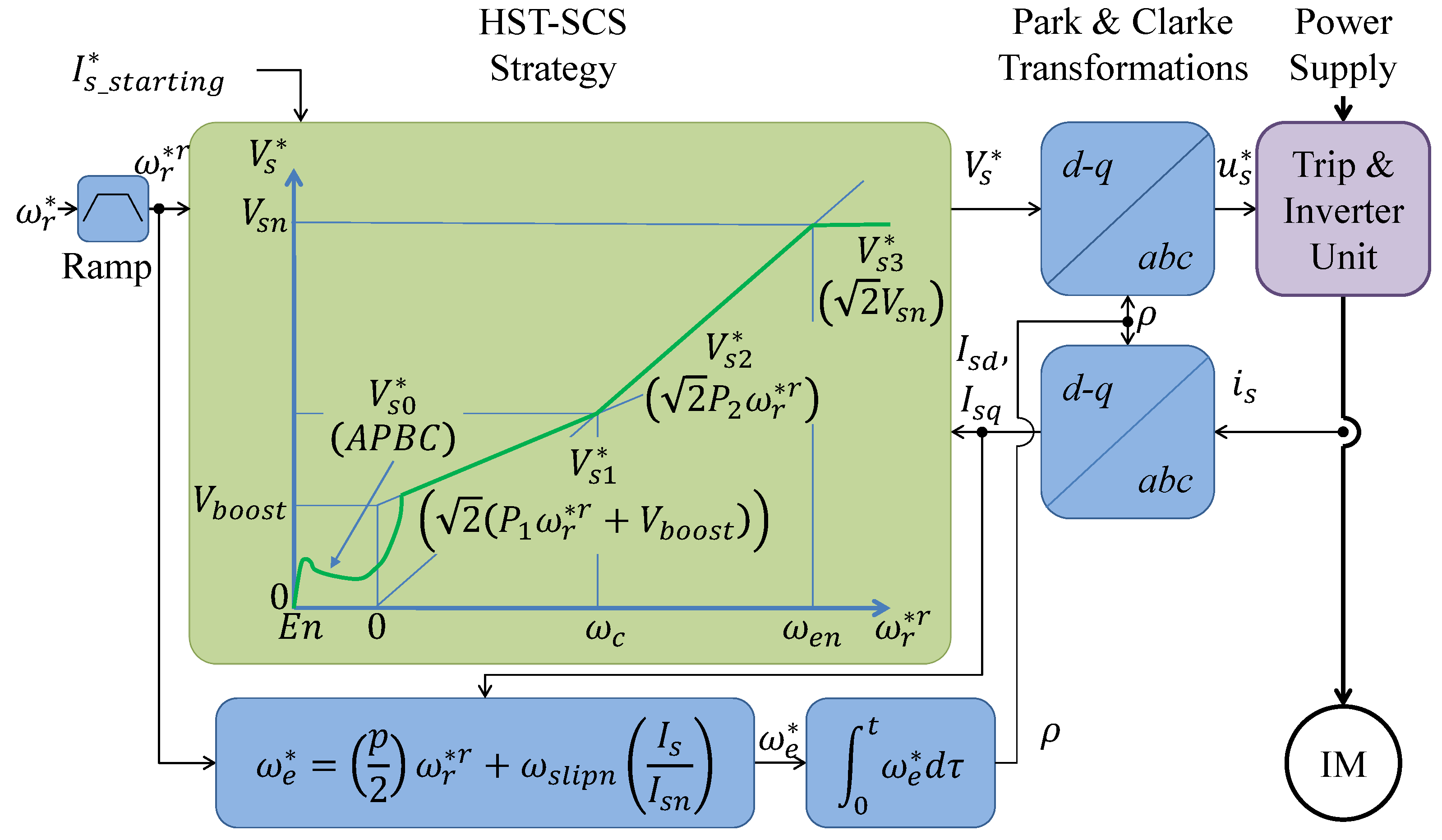
Figure 2 presents the basic HST-SCS block diagram [16].
The basic HST-SCS follows the required rotor angular speed ω r * after establishing the required angular electrical frequency ω e * and stator voltage amplitude V s * . It takes steady-state nominal variable values from the motor nameplate for configuring purposes. For instance, the rated current per phase I s n , the rated voltage per phase V s n , the number of poles p, the electrical frequency f n , and the rated rotor angular speed ω r n . These last two allow calculating the nominal slip speed ω s l i p n as follows [6]:
ω s l i p n = ω e n p 2 ω r n ,
which allows computing the actual ω s l i p n for the required ω r * joint to I s n and the actual I s . This last one is an RMS value obtained from the instantaneous stator components I s d and I s q , considered as sinusoidal signals, and as follows:
I s = I s d 2 + I s q 2 2 .
The required stator voltage amplitude (3) switches from different voltages curves V s 0 * , V s 1 * , V s 2 * , and V s 3 * [16] after enabling the VSD ( E n = 1 ), as the following describes:
V s * = V s 0 * ( APBC ) if E n = 1 & V s 0 * < V s 1 * V s 1 * = 2 ( P 1 ω e * + V b o o s t ) if V s 2 * < V s 1 * V s 0 * V s 2 * = 2 P 2 ω e * if V s 1 * < V s 2 * V s 3 * V s 3 * = 2 V s n if V s 2 * > V s 3 * .
Moreover, the required stator voltage amplitude (3) alternates after applying the transformations of Park e j ρ [23] and Clarke [24], detailed in [25]. In [16], the voltage curve V s 0 * of (3) aims to keep a constant stator flux magnitude at the start via the following APBC that regulates the starting stator current [16]:
Theorem 1
([16]). After applying the following normalized-APBC to the IM d-q model:
V s 0 = θ T Ω ¯ θ T = 0 t Γ e Ω ¯ T d τ , with e = I s _ s t a r t i n g * I s n , and I s _ s t a r t i n g * = ξ I s n Ω ¯ = 100 v v n Ω ¯ 1 I s d I s n Ω ¯ 2 I s q I s n Ω ¯ 3 ω e * I s q ω e n I s n Ω ¯ 4 ω r * I s d ω r n I s n Ω ¯ 5 ω r * I s q ω r n I s n Ω ¯ 6 T , Γ = ϵ 1 + 100 2 , and ; θ T ( 0 ) = 0 v = K e with K = 5 m τ e l e c t , τ e l e c t = τ m e c h 10 , and τ m e c h = 1 2 J m , and ϵ 0.1 , 10 , m 0.1 , 10 , ξ 0.5 , 1.5 , v n = K ,
it turns the IM into a C 1 passive system from e to the auxiliary variable v. It also guarantees that lim t e = 0 .
This voltage curve V s 0 * uses the stator flux magnitude dependence on the magnetizing current, | Φ s |   = L m | i m | , considering the incoming expression [15,16]:
| Φ s |   = L m | i m |   = L m | i s j L m R r ω s l i p + j L r i s i r |   = L m | i s R r ω s l i p + j L r R r ω s l i p + j L r | ,
where L r is the rotor leakage inductance, L m is the magnetizing inductance, and R r and L r are the stator resistance and inductance, respectively. Moreover, i s , i r , and i m are the stator, rotor, and magnetizing phase currents, respectively.
Furthermore, regulating the starting stator current i s guarantees a high starting electromagnetic torque capability as the following describes [15,16]:
T e m = 3 p 2 | j L m R r ω s l i p + j L r | 2 K p | i s | 2 .
The boost voltage curve V s 1 * and the V / f voltage curve V s 2 * , from Figure 1 and Figure 2, are basically proportional controllers, adjusted as follows:
P 1 = V s n ω e n V b o o s t ω c and P 2 = V s n ω e n ,
The voltage curves V s 1 * and V s 2 * aim to keep a constant stator flux magnitude | Φ s | but using its dependence on the stator voltage and angular electrical frequency ratio | Φ s | | u s | ω e * . This comes from the steady-state IM equivalent circuit per phase after applying Kirchhoff’s stator voltage law [3,15,16,25] and neglects the stator impedance voltage drop, as follows:
u s * = R s i s + j ω e * L s i s d r o p v o l t a g e 0 + j ω e * L m i m Φ s | Φ s | | u s | ω e * ,
where R s and L s are the stator resistance and leakage inductance, respectively. Moreover, u s is the stator phase voltage. Finally, V s 3 * prevents the IM from operating over the nominal stator voltage, V s n , and protects it.
Remark 1.
The APBC (4) proposed in [16] considers the required rotor angular speed instead of the actual rotor angular speed, i.e., ω r = ω r * , and effectively regulates the stator current around the start. However, the following section extends its efficacy after considering the actual speed and a cascade APBC.

3. Proposed CL HST-SCS for IM

In this section, based on the following IM dynamical d-q model described, this paper proposes a cascade N-APBC and applies it to HST-SCS.

3.1. Proposed Cascade N-APBC for Nonlinear Systems

The IM dynamical d-q model is a class of nonlinear systems defined as follows:
y ˙ i ( t ) = α a ( y i , y o ) + β b ( y i , y o ) u i ( t ) , y ˙ 0 ( t ) = γ c ( y i , y o ) + δ d ( y i , y o ) y i ( t ) , z ˙ ( t ) = q ( z , y ) .
Here, y i ( t ) , y o ( t ) are the inner and outer outputs; the inner and outer control inputs are u i ( t ) , y i ( t ) * . The unknown parameters are β , δ , α , and γ 1 x n . The known nonlinear functions are b ( y i , y o ) , d ( y i , y o ) , a ( y i , y o ) , and c ( y i , y o ) m , with b ( y i , y o ) 0 and d ( y i , y o ) 0 . Moreover, it has a bounded-input bounded-output (BIBO) internal dynamics z ( t ) l .
The following Theorem 2 extends a cascade APBC [21] for nonlinear systems of the form (9).
Theorem 2.
After applying the following cascade N-APBC to the nonlinear system (9), it turns the IM into a C 1 passive system from e o and e i to the auxiliary variables v 0 and v i , respectively, with e o ( t ) = y o * ( t ) y o ( t ) and e i ( t ) = y i * ( t ) y i ( t ) . It also guarantees that lim t e o = 0 and lim t e i = 0
Inner Loop u i ( t ) = b ( y i , y o ) 1 θ i ( t ) T Ω i ( t ) ¯ , adaptive controller θ i T = 0 t Γ i e i Ω i ( t ) ¯ T d τ , with θ i T ( 0 ) = 0 , adaptive controller parameter Ω i ( t ) ¯ T = 100 a ( y i , y o ) a n a ( y i , y o ) ¯ v i ( t ) K i v i ( t ) ¯ , normalized information vector with Γ i = ϵ i 1 + 100 2 , normalized fixed gain and v i ( t ) = K i e i + y ˙ i * ( t ) , inner auxiliary variable
Outer Loop y i * ( t ) = d ( y i , y o ) 1 θ o ( t ) T Ω o ( t ) ¯ , adaptive controller θ o T = 0 t Γ o e o Ω o ( t ) ¯ T d τ , with θ o T ( 0 ) = 0 , adaptive controller parameter Ω o ( t ) ¯ T = 100 c ( y i , y o ) c n c ( y i , y o ) ¯ v o ( t ) K i v o ( t ) ¯ , normalized information vector with Γ 0 = ϵ o 1 + 100 2 . normalized fixed gain and v o ( t ) = ξ 1 K i e o + y ˙ o * ( t ) , outer auxiliary variable
Here, y o * ( t ) is the desired trajectory. The normalization factors a n , c n , y n , and y n * correspond to the maximum operational range of a ( y ) , c ( y ) , y ( t ) , and y * ( t ) , respectively. The normalized information vectors consider these factors and multiply by 100, normalizing a 100 range. Hence, the fixed-gains Γ i , Γ 0 , and + have a form ϵ 1 + ξ 2 [16], with ξ = 100 . Then, these use the term 1 1 + 100 2 for a fast tuning, assuring a reasonable operating range and the design parameters ϵ i , ϵ o 0.1 , 10 , which allows a fine-tuning adjustment. Moreover, ξ 3 , 10 assures an inner loop ξ times faster than the outer loop for the cascade proper functioning. Appendix A contains the stability proof of Theorem 1.
The following section applies Theorem 2 to the IM and describes the proposal details.

3.2. Cascade N-APBC Applied to HST-SCS for IM

Figure 3 shows the proposed CL HST-SCS block diagram for IM.
It has a similar control scheme to Figure 2 but adjusts the voltage curve V s 0 * after applying the proposed cascade N-APBC (10, 11) to the IM model, once considering as unknown its nonlinear parameters α , β , γ , and δ , and its known functions a ( y ) , b ( y ) , c ( y ) , and d ( y ) . Hence, the proposal also uses (1) to calculate the slip. However, it establishes the scalar required stator voltage V s * (3), replacing the adaptive controller (4) conforming the voltage curve V s 0 * with the following proposed controller for V s 0 * .
Inner Loop V s 0 = θ i T Ω ¯ i , where θ i T = 0 t Γ i e i Ω ¯ i T d τ , Ω ¯ i = 100 v i K i Ω ¯ i 1 I s d I s n Ω ¯ i 2 I s q I s n Ω ¯ i 3 ω e * I s q ω e n I s n Ω ¯ i 4 ω r I s d ω r n I s n Ω ¯ i 5 ω r I s q ω r n I s n Ω ¯ i 6 T , with Γ i = ϵ i 1 + 100 2 , θ i T ( 0 ) = 0 , and v i = K i e i + I ˙ s d * , with K i = 5 m τ e l e c t , τ e l e c t = τ m e c h 10 , τ m e c h = 1 2 J m , here , e i = I s d * I s d .
Outer Loop I s d * = S i g n ( θ o T Ω ¯ o ) θ o T Ω ¯ o + I s _ s t a r t i n g * where θ o T = 0 t Γ o e o Ω ¯ o T d τ , Ω ¯ o = 100 v o K i Ω ¯ o 1 ω r ω r n Ω ¯ o 2 1 Ω ¯ 03 T , with Γ o = ϵ o 1 + 100 2 , θ o T ( 0 ) = 0 , v o = ξ 1 K i e o + ω ˙ r * , and e o = ω r * ω r .
Here, the adaptive controller parameters are θ i 6 and θ o 3 . The fixed-gains are Γ i , Γ o + depending on the design parameter ϵ o , ϵ i 0.1 , 10 . The normalized information vectors are Ω ¯ i 6 and Ω ¯ o 3 .
The CL HST-SCS considers that the IM dynamical d-q model has the form of (9). Here, the outputs are y i ( t ) = I s d , y o ( t ) = ω r , and the control inputs are u i ( t ) = V s d , u o ( t ) = | I s | 2 . The unknown parameters are α = A 1 u p p e r 1 A 2 u p p e r 5 , β = 1 σ L s , γ = b p J 1 J T l 2 , and δ = | j L m R r ω s l i p + j L r | 2 . Additionally, the known nonlinear functions are a ( y ) = I s d I s q ω e * I s q p 2 ω r I s q p 2 ω r I s q T 5 , b ( y ) = 1 , c = ω r 1 T 2 , and d = 3 p 2 . Moreover, the internal dynamics are z ( t ) = I s q Φ r d Φ r q T 3 , defined as follows:
q ( z , y ) = A 1 l o w e r I s d I s q ω e * I s d + A 2 l o w e r p 2 ω r I s d d I s q + β V s q C Φ n d Φ r q + d I s d I s q .
Here, Φ r d and Φ r q are the rotor flux direct and quadrature components, respectively. The mechanical viscous damping is b p , the motor-load inertia is J, and the load torque is T l . Moreover, the vector A 1 u p p e r 2 and A 1 l o w e r 2 are upper and lower rows of the matrix A 1 , respectively. The vectors A 2 u p p e r 2 and A 2 l o w e r 2 are the upper and lower rows of matrix A 2 , respectively. Moreover, C, d, A 1 , and A 2 are defined as follows [16]:
C = R r L r ω s l i p ω s l i p R r L r , d = R r L m L r , A 1 = R s σ L s 0 0 R s σ L s L m R r σ L s L r 2 d C 1 , A 2 = L m R r σ L s L r d 0 1 1 0 C 1 .
Furthermore, σ is the leakage or coupling coefficient, given by σ = 1 L m 2 / ( L r L s ) , and R s is the stator transient resistance, with R s = R s + ( L m 2 R r ) / ( L r 2 ) .
The following Algorithm 1 contains the pseudocode of the proposed CL HST-SCS. Here, the required stator voltage amplitude (3) considers the proposed cascade-APBC (12) and (13).
Algorithm 1 Pseudocode of the required voltage and frequency for the CL HST-SCS
Require: ω r * , I s _ s t a r t i n g * , E n (Reference and Input Signal)
Require:p, J m , f n , ω r n , I s n , V s n , ω c , m, ϵ i , ϵ i , ξ , r a m p _ r a t e (Configuring Parameters)
Require: ω r , I s d , I s q (Measurements)
Ensure: Required Stator Voltage V s * and electrical frequency ω e *
  • ω e * Calculus
  •       ω e n = 4 π f n p ; ω s l i p n = ω e n p 2 ω r n ; I s = I s d 2 + I s q 2 2 ; ω r * r = Ramp ( ω r * , r a m p _ r a t e ) ;
  •      ω e * = p 2 ω r * r + ω s l i p n I s I s n ;
  • V s 0 Computing
  •         Outer Loop
  •         Compute:  e o = ω r * ω r ; τ m e c h = 1 2 J m ; τ e l e c t = τ m e c h 10 ; K i = 5 m τ e l e c t ;
  •                        v o = ξ K i e o + ω ˙ r * ; Γ o = ϵ o 1 + 100 2 ;
  •                        Ω ¯ o = 100 v o ξ K i Ω ¯ o 1 ω r ω r n Ω ¯ o 2 1 Ω ¯ 03 T ; θ o T = 0 t Γ o e o Ω ¯ o T d τ ;
  •                        I s d * = S i g n ( θ o T Ω ¯ o ) θ o T Ω ¯ o + I s _ s t a r t i n g * ;
  •         Inner Loop
  •         Compute:  e i = I s d * I s d ; v i = K i e i + I ˙ s d * ; Γ i = ϵ i 1 + 100 2 ;
  •                        Ω ¯ i = 100 v i K i Ω ¯ i 1 I s d I s n Ω ¯ i 2 I s q I s n Ω ¯ i 3 ω e * I s q ω e n I s n Ω ¯ i 4 ω r I s d ω r n I s n Ω ¯ i 5 ω r I s q ω r n I s n Ω ¯ i 6 T ;
  •                        θ i T = 0 t Γ i e i Ω ¯ i T d τ ; V s 0 = θ i T Ω ¯ i ;
  • V s 1 Computing
  •         Compute:  V s 1 * = 2 ( P 1 ω e * + V b o o s t ) ;
  • V s 2 Computing
  •         Compute:  V s 2 * = 2 P 2 ω e * ;
  • V s 3 Computing
  •         Compute:  V s 3 * = 2 V s n ;
  • Voltage Curve Selection
  • ifEn = 1 and  V s 0 * < V s 1 *  then
  •      V s * = V s 0 *
  • else if V s 2 * < V s 1 * V s 0 * then
  •      V s * = V s 1 *
  • else if V s 1 * < V s 2 * V s 3 * then
  •      V s * = V s 2 *
  • else V s 2 * > V s 3 *
  •      V s * = V s 3 *
  • end if
The following section describes the proposal’s experimental results.

4. Comparative Experimental Results

This section describes the test bench used to validate the proposal, the experimental setup, and the comparative results.

4.1. Test Bench Characteristics

Figure 4 illustrates the test bench used for the comparative experimental results, considering the basic HST-SCS and the CL HST-SCS. The programming of these strategies uses Simulink version 8.9, Matlab R2017a running on PC. Both consider a pulse width modulation (PWM) switching at 8 kHz. Once finished, the PC downloads them via a UTP cable to the control platform. It is a real-time simulator controller OPAL-RT 4510 v2 giving the trip pulses to a two-level inverter unit feeding an IM-load assembly with the parameters of Table 1. The power supply feeds the inverter through a variac.
Remark 2.
The used test bench is based on a double-edge naturally sampled PWM with a two-level voltage source inverter [26], which inherently produces a bipolar switching pattern at the converter outputs. However, the control proposal could also be implemented using the space vector modulation method to improve the harmonic content further, especially for higher modulation indexes when the machine operates around the rated speed [26,27]. The proposed CL HST-SCS could also be implemented in a three-level converter using unipolar PWM.
From this Table 1, the following parameters are calculated: the rated electrical frequency ω e n = 4 π f p = 314.16 rad/s and the rated electromagnetic torque T n = 1000 P n ω r n = 49.2 Nm.
Remark 3.
Please note that IM parameter values, such as L r , L s , L m , R r , and R s , are unknown. Moreover, their knowledge is unnecessary for the proposed CL HSTSCS configuring. Not even the torque-speed characteristic of the feed IM is needed. Table 1 shows the only required IM information taken from the motor nameplate and datasheet.
The following section describes the experimental testing setup.

4.2. Experimental Setup

The same testing applies to both strategies, the basic HST-SCS [16] and CL HST-SCS. It considers the IM has a nominal torque load (set by a prony brake), a 6-second duration test, enabling the VSDs at 0.3 s, and applying a step speed command of 200 rpm, 100 rpm, 1450 rpm, 1300, and 1150 rpm, at times 1 s, 1.4 s, 1.7 s, 4 s, and 5 s, respectively. The prony brake adjustment is 49.6 Nm at the rated speed of 1455 rpm. As a result, the load torque equals 49.2 Nm (the rated torque) at 200 rpm and 100 rpm, 49.8 Nm at 1455 rpm, 49.6 Nm at 1300 rpm, and 49.4 NM at 1100 rpm.
Table 2 presents the tuning parameters.
The following section describes the obtained results.

4.3. Comparative Experimental Results
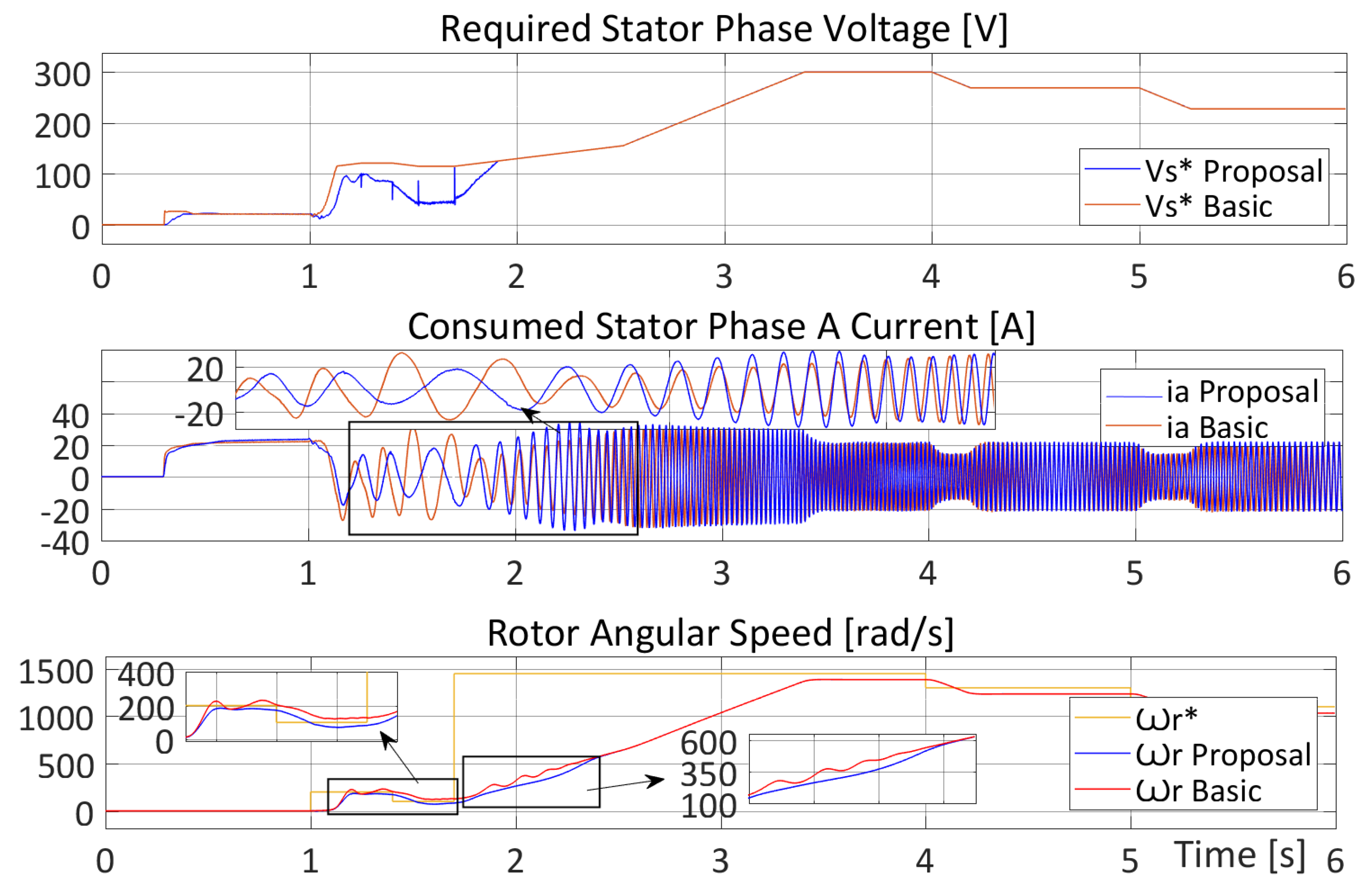
Figure 5 and Figure 6 show the previous HST-SCS [16] and CL HST-SCS oscilloscope waveforms, respectively. Both figures exhibit the applied line Voltage u s a b and the consumed stator phase currents i s a , i s b , and i s c around 5.1 s.
Below, Figure 7 shows comparative graphics obtained via the OPAL-RT measurements. It displays the consumed stator phase A current i s a joint to the required stator phase voltage amplitude V s * , and the rotor angular speed ω r * versus ω r for the basic and CL HST-SCS.
The required stator phase voltage V s * in Figure 7 shows that CL HST-SCS and HST-SCS apply DC voltage after enabling the VFD and until 1 s. When the IM starts rotating, the HST-SCS keeps using the adaptive starting controller, between 1 s and 1.2 s. Later, it switches to the boost curve, active from 1.1 s to 2.5 s. Finally, the V / f curves operate from 2.5 s until the end.
Figure 7 evidences that required stator phase voltage is lower for the CL HST-SCS. Moreover, the V s 0 voltage curve applies for a more extended time, from the start to 1.9s, for the CL HST-SCS. As a result, the CL HST-SCS assures HST not only for starting but almost up to 500 rpm.
The consumed stator phase A current described in Figure 7 displays similarly consumed DC stator current magnitudes (starting currents) for both strategies. These consume 21.9A for starting; the nominal stator current 2 I s n . However, it is lower for the CL HST-SCS when starting. After 2.6 s, consumption is similar for the CL HST-SCS and HST-SCS. Figure 7 shows the details.
The actual rotor speed follows the required rotor speed for both HST-SCS strategies. However, the CL HST-SCS has a smoother transient behavior than HST-SCS under 600 rpm. This last one shows a more oscillatory behavior. CL HST-SCS and HST-SCS have similar transient behavior and steady-state accuracy for higher speed references. These last ones are 3.0% for 1455 rpm, 3.8% for 1300 rpm, and 4.1% for 1150 rpm.
The following section describes the conclusions.

5. Conclusions

This paper studies a basic HST-SCS and a CL HST-SCS. Both strategies assure HST with low current consumption compared with the standard SCS [16]. They all follow the required speed. Moreover, they have a simple control scheme without parameters estimation nor variable observers, but only depend on the IM nameplate and datasheet for their configuring.
Comparative experiments were performed on a test bench. These show that the CL HST-SCS delivers high torque capabilities beyond the starting. Thus, CL HST-SCS has a smoother transient behavior than HST-SCS under 600 rpm.
The proposal of a cascade N-APBC for nonlinear systems encompassing IM allows for obtaining the CL HST-SCS. It considers normalized inner and outer adaptive loops expanding [21]. Moreover, it further extends the APBC [15], normalized in [16], to reduce trial and error APBC adjustment.
The proposed CL HST-SCS contributes to expanding the standard SCS low-performance applications. Not only moving blowers, fans, and centrifugal pumps, but other loads that need a starting torque of 100% rated torque. Future work will consider developing real-time simulations for a higher power IM, including multilevel inverters and SVM modulation.

Author Contributions

Conceptualization, methodology, writing—original draft preparation, and visualization, J.C.T.-T.; investigation, formal analysis, supervision, project administration, data curation, and resources and funding acquisition, J.C.T.-T. and M.A.D.-M.; validation, software, and writing—review and editing; M.D., C.C.-J. and F.H. All authors have read and agreed to the published version of the manuscript.

Funding

This research was funded by FONDEF Chile, grant ID 17I20338; the applied research project DICYT, grant 082078TT_TEC, Vicerrectoría de Investigación, Desarrollo e Innovación; FONDECYT Chile, grant 1190959. Moreover, it was supported by a 2021 research grant from the Technological Faculty, USACH.

Institutional Review Board Statement

Not applicable.

Informed Consent Statement

Not applicable.

Data Availability Statement

Not applicable.

Conflicts of Interest

The authors declare no conflict of interest.

Abbreviations

The following abbreviations are used in this manuscript:
IMInduction motors
PCPersonal computer
HSTHigh starting torque
SCSScalar control scheme
APBCAdaptive passivity-based controller
MRACModel reference adaptive controller
MIMOMultiple-input multiple-output
BIBOBounded-input bounded-output
FOCField-oriented control
PWMPulse width modulation
IAEIntegral absolute error
VSDVariable speed drives
DCDirect current
SVMSpace vector modulation
Main Notation
The following main notations are used in this manuscript:
ω r * , ω r , and ω e * Required rotor, actual, and electrical angular speed
ω r n and ω e n * Rated rotor and required angular speed
ω s l i p and ω s l i p n Actual and rated angular slip speed
e j ρ and e j ρ Park transformation and its inverse
T 3 2 and T 2 3 Clarke transformation and its inverse
V s * Needed stator voltage amplitude
V s α β * Needed two-phase alternating instantaneous voltage in α - β coordinates
u s * Needed three-phasic alternating instantaneous voltage
V s n Rated voltage per phase (RMS value)
I s n and I s Rated and actual current per phase (RMS value)
I s d and I s q Actual stator current direct and quadrature component per phase
i s , i r , and i m Stator, rotor, and magnetizing instantaneous current
P F n Rated power factor
f n Rated electrical frequency in Hz
pNumber of poles
E n VFD enable
V b o o s t boost voltage
V s 0 * Starting voltage curve for HST
V s 1 * Boost voltage curve
V s 2 * V/f voltage curve
V s 3 * Weakening flux zone voltage curve
P 1 and P 2 Controller parameters for V s 1 * and V s 2 * , respectively
ω c Cut angular frequency, switching point between V s 1 * and V s 2 *
R s and R r Stator and rotor resistance
L s and L r Stator and rotor leakage inductance
L s , L r , and L m Stator, rotor, and magnetizing inductance
σ Leakage or coupling coefficient, given by σ = 1 L m 2 / ( L r L s )
R s Stator transient resistance, with R s = R s + ( L m 2 R r ) / ( L r 2 )
| Φ s | Stator flux magnitude

Appendix A. Stability Proof of Theorem 1

Proof of Theorem 1. 
Adding and subtracting the terms K i e i + y ˙ i * and K o e o + y ˙ o * into the right side of the first and fourth equations of (9), considering that e ˙ i ( t ) = y ˙ i ( t ) y ˙ i * ( t ) and e ˙ o ( t ) = y ˙ o ( t ) y ˙ o * ( t ) , and making some algebraic arrangements, it is obtained that
e ˙ i ( t ) = K i e i + β θ i * T Ω ¯ i u i ( t ) * e ˙ o ( t ) = K o e o + δ θ o * T Ω ¯ o I s d * 2 z ˙ ( t ) = q ( z , y ) .
where θ i * T = β 1 Ω i n 100 α 1 ( m + 1 ) and θ o * T = δ 1 Ω 0 n 100 γ 1 ( m + 1 ) are the normalized ideal controller parameters. The S i g n ( β ) = 1 and S i g n ( δ ) = 1 (are positive). All parameters are assumed to be unknown and constant, which may have a slow variation. Thus, the authors substitute (10) and (11) into (A1), and define the controller parameters errors as Φ i = θ i * T θ i and Φ o = θ o * T θ o (which implies that Φ ˙ i ( t ) = θ ˙ i ( t ) and Φ ˙ o ( t ) = θ ˙ o ( t ) as θ i * T and θ o * T are constant vectors). Moreover, considering stable internal dynamics, as the state variables I s q , Φ r d , and Φ r q are the bounded-input bounded-output (BIBO), the obtained error model is
e ˙ i ( t ) = K i e i + b Φ i T Ω ¯ i Φ ˙ i T ( t ) = Γ i e i Ω ¯ i T with Γ i + e ˙ o ( t ) = K o e o + 1 J K p Φ o T Ω ¯ o Φ ˙ o T ( t ) = Γ o e o Ω ¯ o T with Γ o + .
The obtained error model (A2) has the following associated Lyapunov function:
V e i , e 0 , Φ i , Φ o = 1 2 e i 2 + e o 2 + 1 2 T r a c e β Φ i T Γ i 1 Φ i + δ Φ o T Γ o 1 Φ o .
Taking the time derivative of this Lyapunov function we have:
V ˙ e i , e 0 , Φ i , Φ o = e i e ˙ i + e o e ˙ o + T r a c e β Φ ˙ i T Γ 1 Φ i + T r a c e δ Φ ˙ o T Γ o 1 Φ o .
The time derivatives of e i , e o , Φ i , and Φ o from (A2) are substituted into this last expression. Moreover, the two vectors’ property, where a T b = T r a c e ( a b T ) , is considered to write the terms e i β Φ i T Ω i and e o δ Φ o T Ω o into the trace as T r a c e ( β e i Ω i T Φ i ) and T r a c e ( δ e o Ω o T Φ o ) , respectively. Finally, rearranging and canceling terms due to β = β and δ = δ , after knowing both have a positive sign, we obtain:
V ˙ e i , e 0 , Φ i , Φ o = K i e i 2 K o e o 2 .
As can be seen in this last Equation (A5), the first time derivative of the Lyapunov function (A3) is negative semidefinite; thus, the autonomous system (A2) is stable. Moreover, as e i , e o , Φ i , and Φ o are stables, with bounded Ω i and Ω o , then e i ˙ and e o ˙ are bounded. Integrating both sides of (A5), it can be concluded that e 2 . Hence, according to Barbalat′s Lemma, the error e is asymptotically stable. This concludes the proof.  □

References

  1. Bose, B. Modern Power Electronics and AC Drives; Eastern Economy Edition; Prentice Hall PTR: Hoboken, NJ, USA, 2002. [Google Scholar]
  2. Hannan, M.; Ali, J.A.; Mohamed, A.; Hussain, A. Optimization techniques to enhance the performance of induction motor drives: A review. Renew. Sustain. Energy Rev. 2018, 81, 1611–1626. [Google Scholar] [CrossRef]
  3. Vas, P. Electrical Machines and Drives: A Space-Vector Theory Approach; Oxford University Press: New York, NY, USA, 1992. [Google Scholar]
  4. Varma, G.H.K.; Barry, V.R.; Jain, R.K. A Total-Cross-Tied-Based Dynamic Photovoltaic Array Reconfiguration for Water Pumping System. IEEE Access 2022, 10, 4832–4843. [Google Scholar] [CrossRef]
  5. Carbone, L.; Cosso, S.; Kumar, K.; Marchesoni, M.; Passalacqua, M.; Vaccaro, L. Stability Analysis of Open-Loop V/Hz Controlled Asynchronous Machines and Two Novel Mitigation Strategies for Oscillations Suppression. Energies 2022, 15, 1404. [Google Scholar] [CrossRef]
  6. Control-Techniques. Commander SE Advanced User Guide; Part Number: 0452-0049, Issue Number 3, Control Techniques Drives Limited: Stafford Park, UK, 2002. [Google Scholar]
  7. Otkun, Ö. Scalar Speed Control of Induction Motors with Difference Frequency. J. Polytech. 2019, 23, 267–276. [Google Scholar] [CrossRef]
  8. Duranay, Z.; Guldemir, H.; Tuncer, S. Implementation of a V/f Controlled Variable Speed Induction Motor Drive. EMITTER Int. J. Eng. Technol. 2020, 8, 35–48. [Google Scholar] [CrossRef]
  9. Koga, K.; Ueda, R.; Sonoda, T. Constitution of V/f control for reducing the steady-state speed error to zero in induction motor drive system. IEEE Trans. Ind. Appl. 1992, 28, 463–471. [Google Scholar] [CrossRef]
  10. Munoz-Garcia, A.; Lipo, T.; Novotny, D. A new induction motor V/f control method capable of high-performance regulation at low speeds. IEEE Trans. Ind. Appl. 1998, 34, 813–821. [Google Scholar] [CrossRef] [Green Version]
  11. Wang, C.C.; Fang, C.H. Sensorless scalar-controlled induction motor drives with modified flux observer. IEEE Trans. Energy Convers. 2003, 18, 181–186. [Google Scholar] [CrossRef]
  12. Smith, A.; Gadoue, S.; Armstrong, M.; Finch, J. Improved method for the scalar control of induction motor drives. IET Electr. Power Appl. 2013, 7, 487–498. [Google Scholar] [CrossRef] [Green Version]
  13. Lee, K.; Han, Y. Reactive-Power-Based Robust MTPA Control for v/f Scalar-Controlled Induction Motor Drives. IEEE Trans. Ind. Electron. 2022, 69, 169–178. [Google Scholar] [CrossRef]
  14. Zhang, Z.; Bazzi, A.M. Robust Sensorless Scalar Control of Induction Motor Drives with Torque Capability Enhancement at Low Speeds. In Proceedings of the 2019 IEEE International Electric Machines Drives Conference (IEMDC), San Deigo, CA, USA, 12–15 May 2019; pp. 1706–1710. [Google Scholar] [CrossRef]
  15. Travieso-Torres, J.C.; Vilaragut-Llanes, M.; Costa-Montiel, Á.; Duarte-Mermoud, M.A.; Aguila-Camacho, N.; Contreras-Jara, C.; Álvarez Gracia, A. New Adaptive High Starting Torque Scalar Control Scheme for Induction Motors Based on Passivity. Energies 2020, 13, 1276. [Google Scholar] [CrossRef] [Green Version]
  16. Travieso-Torres, J.C.; Contreras-Jara, C.; Diaz, M.; Aguila-Camacho, N.; Duarte-Mermoud, M.A. New Adaptive Starting Scalar Control Scheme for Induction Motor Variable Speed Drives. IEEE Trans. Energy Convers. 2022, 37, 729–736. [Google Scholar] [CrossRef]
  17. Travieso-Torres, J.C.; Duarte-Mermoud, M.A. Normalized Model Reference Adaptive Control Applied to High Starting Torque Scalar Control Scheme for Induction Motors. Energies 2022, 13, 1276. [Google Scholar]
  18. Narendra, K.; Annaswamy, A. Stable Adaptive Systems; Dover Books on Electrical Engineering; Dover Publications: New York, NY, USA, 2012. [Google Scholar]
  19. Travieso-Torres, J.C.; Duarte-Mermoud, M.; Sepúleveda, D. Passivity-based control for stabilization, regulation and tracking purposes of a class of nonlinear systems. Int. J. Adapt. Control. Signal Process. 2007, 21, 582–602. [Google Scholar] [CrossRef]
  20. Dini, P.; Saponara, S. Design of Adaptive Controller Exploiting Learning Concepts Applied to a BLDC-Based Drive System. Energies 2020, 13, 2512. [Google Scholar] [CrossRef]
  21. Travieso-Torres, J.C.; Duarte-Mermoud, M.A.; Estrada, J.L. Tracking control of cascade systems based on passivity: The non-adaptive and adaptive cases. ISA Trans. 2006, 45, 435–445. [Google Scholar] [CrossRef] [Green Version]
  22. Ganesan, S.; David, P.W.; Balachandran, P.K.; Samithas, D. Intelligent Starting Current-Based Fault Identification of an Induction Motor Operating under Various Power Quality Issues. Energies 2021, 14, 304. [Google Scholar] [CrossRef]
  23. Park, R.H. Two-reaction theory of synchronous machines generalized method of analysis-part I. Trans. Am. Inst. Electr. Eng. 1929, 48, 716–727. [Google Scholar] [CrossRef]
  24. O’Rourke, C.J.; Qasim, M.M.; Overlin, M.R.; Kirtley, J.L. A Geometric Interpretation of Reference Frames and Transformations: dq0, Clarke, and Park. IEEE Trans. Energy Convers. 2019, 34, 2070–2083. [Google Scholar] [CrossRef] [Green Version]
  25. Mandic, D.P.; Kanna, S.; Xia, Y.; Moniri, A.; Junyent-Ferre, A.; Constantinides, A.G. A Data Analytics Perspective of Power Grid Analysis-Part 1: The Clarke and Related Transforms [Lecture Notes]. IEEE Signal Process. Mag. 2019, 36, 110–116. [Google Scholar] [CrossRef]
  26. Holmes, D.; Lipo, T. Pulse Width Modulation for Power Converters: Principles and Practice; IEEE Press Series on Power and Energy Systems; Wiley-IEEE Press: Hoboken, NJ, USA, 2003. [Google Scholar]
  27. Holtz, J. Pulsewidth modulation for electronic power conversion. Proc. IEEE 1994, 82, 1194–1214. [Google Scholar] [CrossRef] [Green Version]
Figure 1. Standard SCS block diagram for IM [6].
Energies 15 03489 g001
Figure 2. Basic HST-SCS block diagram for IM [16].
Energies 15 03489 g002
Figure 3. Block diagram of the proposed CL HST-SCS for IM, remarking the differences in red.
Energies 15 03489 g003
Figure 4. Picture of the testing bench.
Energies 15 03489 g004
Figure 5. Oscilloscope voltage and current waveforms for the basic HST-SCS [16].
Energies 15 03489 g005
Figure 6. Oscilloscope voltage and current waveforms for the CL HST-SCS.
Energies 15 03489 g006
Figure 7. Compararative OPAL-RT waveforms of voltage, current, and rotor angular speed.
Energies 15 03489 g007
Table 1. Data from the motor nameplate and datasheet.
SymbolQuantityValues
P n rated output power 7.5 kW
V s n rated phase voltage220 V
I s n rated phase current 15.5 A
P F n rated power factor 0.85
f n rated electrical frequency50 Hz
ppoles number4
ω r n rated rotor angular speed152 rad/s
J m motor inertia (data-sheet)0.2 kgm/s2
Table 2. Tuning parameters for basic HST-SCS [16] versus CL HST-SCS.
Tuning ParameterBasic HST-SCS [16]CL HST-SCS
V b o o s t 40 % V s n 40 % V s n
ω c 50 % ω e n 50 % ω e n
K i 150 J m 150 J m
Γ i , 1 1 + 100 2 1 1 + 100 2
Γ o —– 1 1 + 100 2
I s _ s t a r t i n g * 2 I s n 2 I s n
m11
ϵ i 11
ϵ o —–1
ξ —–3
R a m p _ r a t e 83.8 rad/s83.8 rad/s
Publisher’s Note: MDPI stays neutral with regard to jurisdictional claims in published maps and institutional affiliations.

