Article

Short-Term Electricity Prices Forecasting Using Functional Time Series Analysis

Department of Statistics, Quaid-i-Azam University, Islamabad 45320, Pakistan
*
Author to whom correspondence should be addressed.
These authors contributed equally to this work.
Energies 2022, 15(9), 3423; https://doi.org/10.3390/en15093423
Submission received: 7 April 2022 / Revised: 28 April 2022 / Accepted: 6 May 2022 / Published: 7 May 2022
(This article belongs to the Special Issue Forecasting and Risk Management Techniques for Electricity Markets)

Abstract

:
In recent years, efficient modeling and forecasting of electricity prices became highly important for all the market participants for developing bidding strategies and making investment decisions. However, as electricity prices exhibit specific features, such as periods of high volatility, seasonal patterns, calendar effects, nonlinearity, etc., their accurate forecasting is challenging. This study proposes a functional forecasting method for the accurate forecasting of electricity prices. A functional autoregressive model of order P is suggested for short-term price forecasting in the electricity markets. The applicability of the model is improved with the help of functional final prediction error (FFPE), through which the model dimensionality and lag structure were selected automatically. An application of the suggested algorithm was evaluated on the Italian electricity market (IPEX). The out-of-sample forecasted results indicate that the proposed method performs relatively better than the nonfunctional forecasting techniques such as autoregressive (AR) and naïve models.

1. Introduction

In the late 1980s, the worldwide electricity industry had undergone numerous fundamental changes when the state-owned monopolistic structure was restructured into the deregulated and competitive electricity market. The main driving force behind the restructuring of the electricity market was to promote competition among producers, retailers, and consumers by boosting private investments in production, supply, and retail sectors. Liberalization of this sector brought many benefits to the stakeholders in terms of reliable, secure, and economical electricity trading. However, due to electricity’s inherent physical characteristic of non-storability in large volumes, the uncertainty related to electricity prices and demand forecasting increased. In addition, electricity prices and demand series generally exhibit specific features, such as multiple periodicities, long-trend, bank holiday effect, spikes, jumps, etc. In the presence of these features, the forecasting problem is challenging in all three forecasting horizons, i.e., short term, medium term, and long term [1].
In electricity markets, short-term forecasting refers to forecasting electricity prices from a few minutes to a week ahead. Apart from the power scheduling, management, and risk assessment, a short-term forecast is essential for market participants to optimize their bidding strategies. Medium-term forecast generally refers to the forecast made for a few weeks to a few months ahead. It is usually vital for expanding generation plants, scheduling maintenance, developing investment, fuel contracting, bilateral contracting, and hedging strategies. Forecasts ranging from a few months ahead to a few years ahead are commonly referred to as long-term-ahead forecasts. They are used for planning and investment profitability analysis, i.e., making decisions for future investments in power plants, inducing sites, and fuel sources [2,3]. In the literature, short-term forecasting has received greater research attention as the maximum electricity trade takes place in this market.
The literature concerning electricity price forecasting reported several statistical, machine learning, econometric, and hybrid models used to forecast short-term electricity prices [4,5,6,7]. Different linear time series models, including AR, ARMA, ARIMA, SARIMA, and ARIMAX [8,9,10,11,12], and nonlinear time series models, such as NPAR, ARCH, GARCH, and their extensions [13,14,15], are extensively used for forecasting electricity prices. Parametric and nonparametric regression-type models considering multiple, local polynomial, kernel, smoothing spline, and quantile regression are easy to implement and are widely studied in the case of electricity price forecasting [2,16,17,18,19,20,21]. In addition, models based on exponential smoothing including simple, double, and triple Holt’s winters models that account for various periodicities [22,23,24,25,26,27] are often used for forecasting purposes. Artificial intelligence models have also been used to predict day-ahead electricity prices [28,29,30,31,32], as well as state-space models [33,34]. Various researchers combined the characteristics of two or more models to build a new model generally referred to as a hybrid model [3,35,36,37,38,39]. Generally, the above-stated models have their own functional and structural form, and the forecasting performance varies from market to market [40].
In the last three decades, technological developments simplified and decreased the cost of data collection and storage processes. Such advancements helped us to examine and record practical life activities in great detail. Examples include curves, images, surfaces, or anything else varying over a continuum. Consequently, classical statistical analysis techniques are inadequate and inefficient due to the large dimensions of data. To analyze such datasets, some suitable statistical methods are required, and functional data analysis (FDA) is one of the prominent methods to tackle such data in an efficient way. The FDA presents the essential statistical background for the analysis of functional variables, where every observation is a continuous function. The application of the FDA exists in almost every field of science, including economics, environment, engineering, energy, etc. [41,42]. In this research work, the application of the FDA is proposed for the electricity market, which is of primary interest for many researchers working in this field, especially after the liberalization of this market.
Given the temporal dependence, the FAR models have been suggested for the time series of trajectories. The autoregressive Hilbertian (ARH) process proposed by [43], also called the FAR model under Hilbert space, is likely the most popular pioneering work that plays an important role in the FDA context.The FAR is an extension of the AR process to infinite-dimensional space and is also used in electricity price forecasting. For example, using functional analysis of variance (FANOVA) and FAR model, Ref. [44] studied the seasonal patterns and improved prediction accuracy for electricity demand time series used from the Nord Pool electricity market. The application of a local linear method with functional explanatory variables was studied by [45]. They compared their proposed approach with the functional Nadaraya–Watson (NW) method and other finite-dimensional nonparametric techniques. For empirical analysis, monthly electricity consumption data of the United States of America (USA) were used, and the results suggest the superior performance of their proposed methods. The forecasting performances of different parametric and nonparametric functional models for electricity demand were studied by [46]. The authors used data from the Italian and British electricity markets and concluded that the nonparametric functional models give superior performance to their parametric counterparts. In another study, Ref. [47] used different functional models and compared their results with the finite univariate dimension (univariate and multivariate) models. Data from four different electricity markets, namely, the Nord Pool electricity market (NP), Pennsylvania–New Jersey–Maryland electricity market (PJM), the Italian electricity market (IPEX), and the British electricity market (APX Power UK), were used, and the results were summarized using different descriptive measures. The results suggested that the functional approach produces better results than the rest. Ref. [48] used the electricity demand curves data from Southern Australia. The author sliced the univariate time series into curves and reduced their dimensionality by applying the functional principal components technique. Finally, the author used univariate time series models to predict short-term electricity demand.
The main aim of this research work is to propose a functional model that can efficiently predict electricity prices. To this end, a method based on a two-components estimation procedure is proposed. The first component, known as the deterministic component, is computed using the additive modeling technique. The stochastic component, on the other hand, is modeled using an FAR( P ) model where the selection of the dimension and lags is automatic. Finally, the model is tested for a whole year to see its forecasting performance. The rest of this paper is organized as follows. Section 2 provides an overview of the preliminaries. Section 3 describes a comprehensive review of the FAR( P ) and functional final prediction error (FFPE). Section 4 provides the application of the proposed method, while Section 5 concludes the study.

2. Functional Modeling

2.1. Preliminaries

Let { Z i ( t ) : i N , t J } be an arbitrary stationary N -dimensional time series where J represents a continuum bounded within a finite interval. For each i, the functional observation Z i belongs to a Hilbert space H = L 2 ( [ 0 , 1 ] , · ) of square integrable functions which is equipped with a norm · induced by the inner product < g , h > = g ( t ) h ( t ) d t . The object Z i ( t ) is referred to as FTS with i as the time index [49,50]. Furthermore, all stochastic functions are defined on a common probability space ( Ω , A , P ) . The notation Z L H p ( Ω , A , P ) is used to indicate E ( Z p ) < for some p > 0 . When p = 1 , Z ( t ) has the mean curve μ ( t ) ; when p = 2 , the covariance operators C ( t , s ) are defined as in Equations (1) and (2) as under
μ ( t ) = E [ Z ( t ) ]
C ( t , s ) = E [ ( Z ( t ) μ ( t ) ) ( Z ( s ) μ ( s ) ) ]
Mercer’s theorem [51] provides the following convenient spectral decomposition of Equation (2):
C ( t , s ) = j = 1 κ j φ j ( t ) φ j ( s )
where φ j denotes the jth orthonormal principal component, and κ j denotes the jth eigenvalue. The principal component scores (PCSs) γ i , j are given by the projection of [ Z i ( t ) μ ( t ) ] in the direction of the jth eigenfunction φ j , i.e., γ i , j = Z i μ , φ j . Based on the separability of the Hilbert space, the Karhunen–Loève (KL) expansion [52,53] of the random function Z ( t ) can be expressed as
Z ( t ) = μ ( t ) + j = 1 γ i , j φ j ( t )
The KL expansion provides the theoretical background for FPCA; see [54,55] for more details about FPCA and its practical demonstration.
Expansion (4) facilitates dimension reduction as the first D terms often provide a good approximation to the infinite sums, and, thus, the information contained in Z ( t ) can be adequately summarized by the jth-dimensional vector ( γ 1 , , γ j ). The approximated processes can be defined as
Z ( t ) = μ ( t ) + j = 1 D γ j φ j ( t ) + ϵ ( t )
where ϵ ( t ) denotes the zero-mean white noise function that captures the variation excluded from the first D leading functional principal components (FPCs). There are different methods available in the literature for choosing the value of D : (i) scree plots or the fraction of variation explained by first few PCSs [56], (ii) using the Akaike information and Bayesian information criteria [57], (iii) cross-validation with one-curve-leave-out or k-fold method [58], or (iv) bootstrap techniques [59].
Once the sample functional data are available, the sample mean can be obtained as
μ ^ ( t ) = 1 N i = 1 N Z i ( t ) , t [ 0 , 1 ] ,
and the sample covariance function is defined as
C ^ ( t , s ) = 1 N 1 i = 1 N Z i ( t ) μ ^ ( t ) Z i ( s ) μ ^ ( s )
Ref. [60] proved that the estimators are consistent for weakly dependent process.

2.2. Functional Autoregressive Model

Autoregressive (AR) models are one of the most popular forecasting models used in time series analysis. In the AR modeling framework, the response variable is linearly dependent on it past p lags with an error term. The theory of AR and more general linear processes in Hilbert spaces is developed in the monograph of [50], containing sufficient technical details. In addition, more relevant information can also be found in [49,61].
Recall a sequence of stationary random curves ( Z i ( t ) , i N ) in L 2 ( [ 0 , 1 ] ) defined in Section 2.1. The functional AR model of order P (FAR ( P ) ) can be written as [50]:
Z i ( t ) μ ( t ) = k = 1 P Ψ k Z i k ( t ) μ ( t ) + ξ i ( t )
where Ψ k ( k = 1 , , P ) are the FAR operators (functional parameters), μ ( t ) is the mean function of Z i ( t ) , Z i k ( t ) denotes k th lag of curve Z i , and ξ i ( t ) is a strong H -white noise with zero mean and finite second moment ( E ξ i ( t ) 2 < ). For the prediction and forecasting of the model given in Equation (8), the following forecasting algorithm is used, which is based on Equations (5)–(7) [62].
  • First, the dimension which is denoted by D is fixed by using the method described in Section 2.3, and the estimated FPC scores are obtained as γ ^ i , j = Z ^ i ( t ) φ ^ j ( t ) d t for each observation Z ^ i ( t ) , i = 1 , , N , j = 1 , , D , and the estimated j-variate FPC scores vectors γ ^ i = ( γ ^ 1 , i , , γ ^ D , i ) t , i = 1 , , N .
  • Next, the order P is fixed using the technique described in Section 2.3 and we fit the vector AR model, VAR( P ), as γ i = k = 1 P Ψ k γ i k + ϵ i for eigenscores vectors to produce forecasting γ ^ N + 1 = ( γ ^ N + 1 , 1 , , γ ^ N + 1 , D ) t . Durbin–Levinson and innovations algorithm can be readily applied here, given the vectors γ ^ 1 , , γ ^ N .
  • In the last step, the multivariate time series are converted back to functional version using the KL theorem Z ^ N + 1 ( t ) = μ ^ ( t ) + γ ^ N + 1 , 1 φ ^ 1 ( t ) + + γ ^ N + 1 , D φ ^ D ( t ) . The FPC scores and sample eigenfunctions result in Z ^ N + 1 ( t ) , which is then used as a one-step-ahead forecast of Z N + 1 ( t ) .
As can be seen, the selection of the dimension D and lags P is an important step in the above algorithm. The following section illustrates how to select the optimal values for these variables.

2.3. Selection of Order and Dimension of FAR( P )

The main goal of the current article is the accurate forecasting through FAR( P ), which requires the appropriate order P selection as well as the dimension D , in such a way that the mean square error (MSE) is minimized.
As the eigenfunctions φ j and the PCS’s γ N , j are uncorrelated, the MSE can be decomposed as
E Z N + 1 Z ^ N + 1 2 = E j = 1 γ N + 1 , j φ j j = 1 D γ ^ N + 1 , j φ j 2 = E Z N + 1 Z ^ N + 1 2 + j = D + 1 κ j
where . 2 denotes the usual l-2 Euclidean norm of vectors. We suppose that the vector Z N is stationary and follows a D -variables vector AR of order P , VAR( P ), that can be written as
Z N + 1 = Φ 1 Z N + Φ 2 Z N 1 + , , + Φ P Z N P + 1 + Y N + 1 .
Ref. [63] showed that ( Y N ) is a white noise process such that
N ( ρ ^ ρ ) D ( 0 , Σ Y Δ P 1 )
where ρ = vec [ Φ 1 , , Φ P ] t and ρ ^ = vec [ Φ ^ 1 , , Φ ^ P ] t is the least squares estimator in vector form, and Δ P = var[vec ( Z P , , Z 1 ) ] and Σ Y = E [ Y 1 , Y 1 t ] . Assume that the ρ ^ are estimated from independent training sample ( X 1 , , X N ) = D ( Z 1 , , Z N ) . It follows then that
E Z N + 1 Z ^ N + 1 2 = E Z N + 1 ( Φ ^ 1 Z N + + Φ ^ P Z N P + 1 ) 2 = E Y N + 1 2 + E ( Φ 1 Φ ^ 1 ) Z N + + ( Φ P Φ ^ P ) Z N P + 1 2 = trace Σ Y + E I P ( Z N t , , Z N P + 1 t ) ( ρ ρ ^ ) 2
For some further derivation by using Equation (10), Ref. [64] showed that Equation (11) can be approximated as
E Z N + 1 Z ^ N + 1 2 N + P D N P D trace ( Σ ^ Y ) + j > D κ j . The suggested functional final prediction error selects order P and dimension D simultaneously by minimizing error term.
f F P E ( P , D ) = N + P D N P D trace ( Σ ^ Y ) + j > D κ j
Using the fFPE method, the suggested forecasting procedure works in a completely data-driven-based way and does not require any subjective specification of parameters. It is specifically important that the choice of D depends upon the sample size N . For more technical details, the interested readers are referred to [64] and the references cited therein.

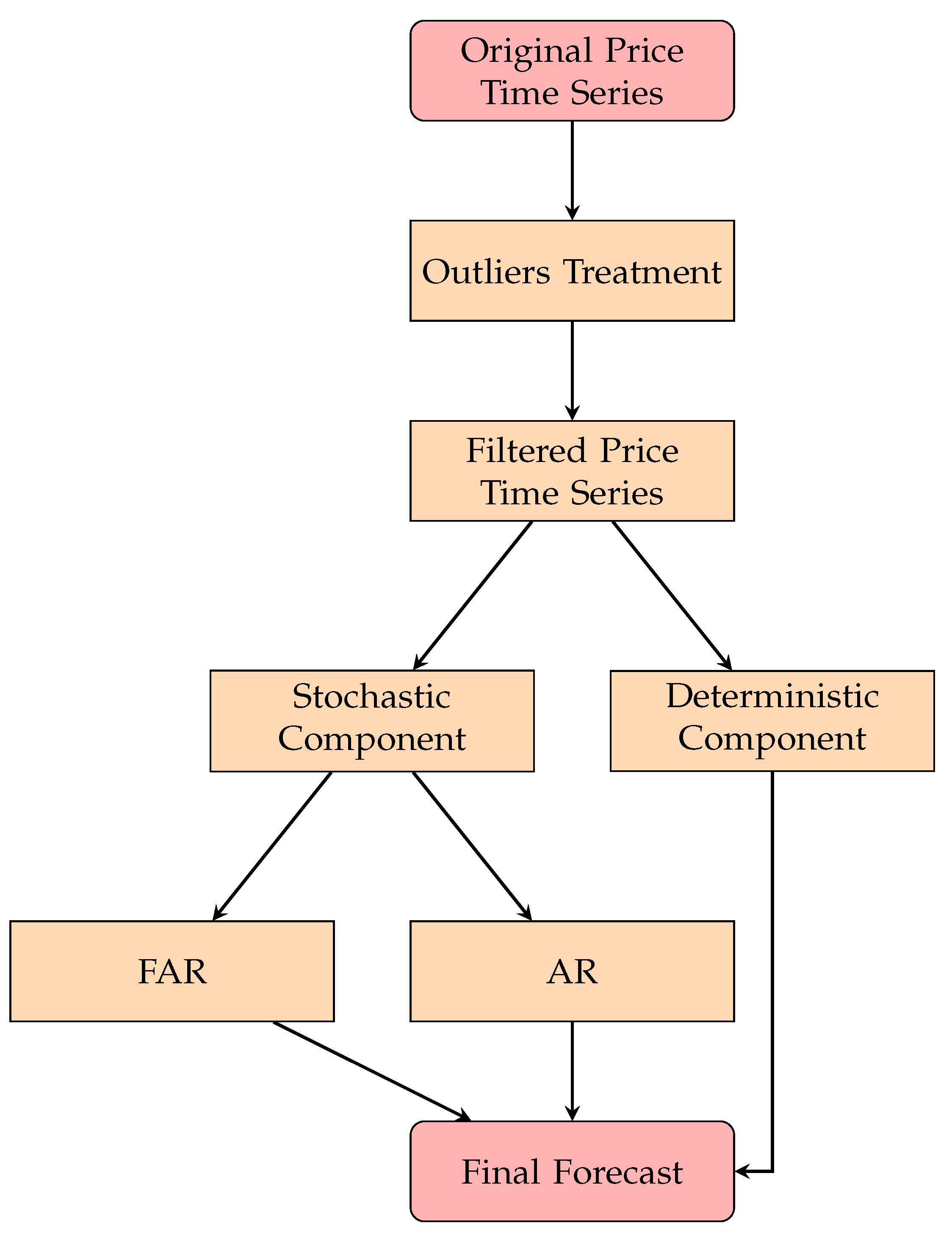
3. Modeling Framework

This section provides the general modeling framework used to model and forecast electricity prices. As described in Section 1, electricity prices exhibit specific features, e.g., extreme values (outliers), multiple periodicities, bank holidays effect, etc. Incorporating these specific features in the model greatly improves the forecasting accuracy [47]. To this end, the price time series is first filtered using the moving window filter on prices discussed in the following section.

3.1. Moving Window Filter on Prices

The identification of outliers, also known as the extreme values, in the data is one of the growing research areas. Various methods and ideas have been used in the literature to detect and impute outliers in the data. The significant developments in terms of outliers detection techniques in time series are suggested by [65,66,67,68]. Generally, the presence of outliers in the original electricity price data can substantially influence most forecasting models, which can result in poor forecasting performance. Therefore, identifying and analyzing outliers in the data is an essential step in constructing a forecasting model.
The moving window filter on price (MFP) [69] is an extension of the standard deviation filter on prices (SFP) technique. The SFP technique is based on the idea that the prices whose absolute deviation is taken from the mean μ ^ and are greater than some multiple of the sample standard deviation σ ^ are referred to as outliers. However, the MFP technique differs from the SFP in the sense that it works out with the rolling window having fixed width of intervals. Using the MFP technique, the original price series is divided into N = T / M parts, where M is the width of the windows. Then, the SFP technique is applied to the first window of the given time series. Next, the window is shifted into the next fixed interval of M width, and the SFP is applied. Finally, the process is repeated until the last window is treated. Our work considers the same predictive interval used in [69], with the width of the window being equal to ten weeks. Thus, the subset of outliers Z , obtained by the MFP with a moving window of width M , is obtained as
Z i o = i = 1 , , N Z τ i : Z τ i μ ^ i 1.64 · σ ^ i τ i ( ( i 1 ) · M + 1 , i · M )
Once the outliers are identified, they are replaced by normal values [70]. In this work, they are replaced by the median value price of the specific window period.

3.2. The Model

Once the filtered price series is obtained, it is modeled using the following model.
Y i = D i + Z i i = 1 , , N
where Y i is the filtered time series and Z i is a stochastic term. The deterministic component captures the long trend, the yearly and weekly periodicity, and the bank holidays effect. Mathematically, it is defined as
D i = l i + y i + w i + b i
where the terms l i , y i , w i , and b i represent the long-term trend, yearly periodicity, weekly periodicity, and bank holidays effect, respectively. In this work, the estimation procedure for the deterministic component described in [71] is used.
Once the deterministic component is estimated, the stochastic component Z i is obtained as
Z i = Y i D i
which is modeled using the aforementioned FAR( P ) and two alternate competing models. The alternate competing models used in this work are the univariate AR(P) model and a naïve benchmark model. The details of the competing models are as below.

3.2.1. Autoregressive (AR) Model

The univariate AR is one of the popular forecasting models used in time series analysis. It is similar to a regression model where the response variable is regressed over its lagged values. More specifically, in the AR modeling, a response variable is linearly dependent on its P lagged (past) values and an error term. Denoted by AR(P), mathematically, it can be written as
Z i = β + k = 1 P α k Z i k + ε i
where Z i is a univariate stationary time series, β is a constant, α k ( k = 1 , , P ) are the autoregressive parameters, and ε i is a white noise process having zero mean and a constant variance. The choice of appropriate lag order selection is one of the most important steps in AR modeling. Different methods, including the Akaike information criterion (AIC) or Bayesian information criterion (BIC), or residual plots, e.g., autocorrelation function (ACF) and partial autocorrelation function (PACF), can be used to determine the lag order to be used in the model. In our work, the ACF and PACF are used, which indicate to use a restricted AR(7) model with α k = 0 for k = 3 , 4 , 5 , 6 . The maximum likelihood estimation (MLE) method is used to estimate the parameters of the above model.
Once both the deterministic and stochastic components are modeled and forecasted, the final forecast is obtained as
Y ^ i + 1 = D ^ i + 1 + Z ^ i + 1 i = 1 , , N .
The flowchart of the proposed general modeling framework is given in Figure 1.

3.2.2. The Naïve Benchmark

This section provides details about a naïve forecasting method that belongs to a similar day technique and has reported greater accuracy than other naïve methods [2]. This method works as follows.
  • To forecast a given day, for example, Thursday, select the day before Thursday, which is Wednesday, and denote it by x .
  • From the validation dataset, select all the Wednesdays (except x ) and compare them with x using the mean absolute error (MAE).
  • Obtain a value of the MAE for each comparison that will result in a vector of the MAE values.
  • Find and locate the smallest value of the MAE in the vector. Once the Wednesday having the lowest MAE is located, use its next day, i.e., Thursday, as the forecast for the concerned Thursday. This process is repeated for all the remaining days of the week.

4. Out-of-Sample Forecast

The dataset used in this empirical study includes electricity prices data called “Prezzo Unico Nazionale (PUN)” from the Italian Electricity Market (IPEX), collected from 1 January 2012 until 31 December 2017. Each day consists of 24 observations, where each observation corresponds to a load period. For modeling and forecasting purposes, we split the data into two periods. The period from 1 January 2012 to 31 December 2016 (1827 days) is used for model estimation. This period is used to optimize the parameters of the models. The out-of-sample period ranges from 1 January 2017 to 31 December 2017 (365 days). This period is used for forecasting the performance of the models. The one-day-ahead out-of-sample forecast is obtained through the window expending technique. In Figure 2, the spot electricity prices series is depicted for six years with a sample of functional (smoothed) curves for a week plotted on the right-hand side. The weekly periodicity is evident in the price time series as the prices profile for working days is relatively different from the non-working days.
The forecasting performance of the proposed and alternative models is compared using three standard descriptive forecast error measures. The point forecast accuracy is evaluated using three standard accuracy measures, namely, mean absolute percentage error (MAPE), MAE, and root mean square error (RMSE). Mathematically, the MAPE, MAE, and RMSE are given as
MAPE = 1 N i = 1 N Z i , j Z ^ i , j Z i , j × 100 MAE = 1 N i = 1 N Z i , j Z ^ i , j RMSE = 1 N i = 1 N [ Z i , j Z ^ i , j ] 2
where N represents the number of observations in the out-of-sample forecasting period, Z i , j denotes the original observed prices of the ith day and jth hour, and Z ^ i , j denotes the forecasted price of the aforementioned day and hour with j = 1 , 2 , , 24 .
In addition, directional forecast statistics can be very beneficial for traders in the electricity market in making investment decisions. These direction moments or turning points can be measured using directional statistic defined as [72]
D s t a t = 1 N i = 1 N α i 100
where
α i = 1 , if ( Z i + 1 , j Z i , j ) ( Z ^ i + 1 , j Z i , j ) 1 0 , otherwise
The electricity prices forecast through the FAR( P ) model have the following steps. In the first step, the moving window filter method was used for the identification and accommodation of outliers. In the second step, a logarithm (log) transformation was performed to stabilize the variance of the series. In the third step, model (14) is applied to the data and the series Z i is obtained using Equation (15). In the fourth step, the Fourier basis functions are used to transform the discrete data into functional data to obtain 2192 daily functional trajectories, say, Z 1 ( t ) , , Z 2192 ( t ) , t J . Once the functional data are obtained, the FAR( P ) model described in Section 2.1 is applied, and one-day-ahead forecasts are obtained for the whole year. In the case of the competing models, the univariate AR model and the naïve benchmark are applied directly to Z i , and the one-day-ahead forecasts are obtained for the whole out-of-sample period.
Figure 3 highlights the population mean function μ ( t ) and the functions obtained by adding and subtracting a suitable multiple of the eigenfunctions to the mean. Such plots are helpful to understand the variability in the direction of certain eigenfunctions. The first eigenfunction is positive, indicating that subjects with positive scores on this component will contribute to obtaining a consistently larger proportion ( 77.1 % ) of the total variation of the data. The second eigenfunction displays an oscillatory behavior, suggesting that subjects with positive scores will have lower electricity prices from midnight till early morning and then slightly more between hours 7 a.m. and 10 a.m., and explain 10.5 % of the total variation of the data. Similarly, the third and fourth eigenfunctions explain 4.8 % and 2.7 % of the total variation of the data, respectively. The first four eigenfunctions collectively explain more than 95 % of the total variability in the electricity prices data.
Concerning the forecasting results for the proposed and alternative models, Table 1 compares the overall forecasting ability of the FAR( P ), AR(7), and naïve models through out-of-sample forecasting errors computed by MAE, MAPE, and RMSE. The table also provides the directional forecasting performance for these models. From the results, it is evident that our proposed functional model performs significantly better than the other competing models. The proposed FAR( P ) models produce MAE, MAPE, and RMSE of 5.16, 8.99, and 8.65, respectively. Although the univariate AR model produces better results than the naïve model, it produces considerably higher forecasting errors compared to the proposed functional model. Looking at the directional forecasting results, note that the value of D s t a t for FAR( P ) is 88.34%, whereas values of 82.96% and 53.64% are obtained in the case of AR and naïve models, respectively. Hence, our proposed functional model performs relatively well compared to the competing models. From the number of forecast direction moments, it can be seen that the FAR( P ) forecast 1525 out of the total 8760 load periods accurately (the“SAME” in Table 1 refers to the absolute difference of the forecasted value minus the actual value to be less than EUR 1), whereas this value for the AR and naïve models is 1272 and 385, respectively. The number of over-forecasted values for FAR( P ) and AR(7) are 3743 and 4084, respectively. Again, the poor performance of the naïve model is evident from the results of the directional forecast.
Table 2 reports the daily forecast accuracy for the electricity prices using different models. From the table, one can see that the FAR( P ) model produces lower forecasting errors compared to the univariate AR(7) and naïve models. Although the forecast errors vary from day to day, they are lower on Thursday and Friday when considering MAPE. The poor performance of the naïve model is evident from this table. The hourly forecast errors for different models are listed in Table 3, which shows that the forecast errors vary throughout the day. Although the FAR( P ) model produces better results on most hours, the AR(7) has better results on two hours when considering the MAPE. It is worth mentioning that the proposed FAR( P ) model performs significantly well during peak hours compared to the competing models. Again, the poor performance of the naïve model is evident from the results.
Finally, the results obtained by our proposed functional model in this study are compared with the results listed in the literature. Here, it is worth mentioning that such a comparison is only to evaluate the performance of our model, as different authors considered different forecasting horizons, different periods, and different error summary measures. Using the Italian electricity market and considering a one-day-ahead forecast, Ref. [2] obtained an MAPE value of 9.74 using the NPAR model, which is significantly higher than our proposed model MAPE value of 8.99. The research work of [73] used the Italian electricity market data, and their proposed model produced an MAE of 8.58, whereas our proposal reported an MAE value of 5.16, 60% lower. For a one-day-ahead forecast, Ref. [70] reported an MAPE value of 9.05, which is slightly higher than our obtained MAPE value. Using an ARX-EGARCH model for the Italian electricity prices time series, Ref. [74] obtained an RMSE of 11.58, whereas our proposed model produced an RMSE value of 8.65. The work of [75] reported RMSE values of 16.72 and 15.79 using ARMA and GARCH models, respectively, significantly higher than our value of 8.65.

5. Conclusions and Future Direction

In today’s competitive electricity market, modeling and forecasting electricity prices are critical for market participants to optimize their strategies. However, electricity prices exhibit specific features, including long-trend, periodicities, spikes or jumps, bank holidays, etc. In the presence of these features, the forecasting problem is a great challenge for researchers. This paper proposes a functional model for modeling and forecasting electricity prices. To this end, the price time series is first treated for the extreme values. The filtered series is then divided into deterministic and stochastic parts. The deterministic part modeled the effects of long-trend, annual, and weekly periodicities, and bank holidays. For the stochastic component, a functional AR model (FAR) is proposed that is capable of automatic selection of lags and dimensions. To evaluate the performance of our proposed model, two alternate models, namely, the univariate AR and a naïve benchmark, are also used in this study. For empirical comparison, data from the Italian electricity market are used and the out-of-sample one-day-ahead forecast errors measured through MAPE, MAE, and RMSE are calculated for a complete year.
The empirical results suggest that the proposed FAR( P ) model is significantly better than the competing model, as it produced considerably lower forecasting errors. Furthermore, the component estimation procedure is highly effective in forecasting electricity prices. Moreover, the directional forecast results suggest that this approach can significantly increase the number of accurate forecasts. Accurate forecasting can be very helpful for the traders (buyers and suppliers) to optimize their bidding strategies to maximize their gains and to use the resources required for electricity generation more effectively. Consequently, this will also benefit the end-user in terms of reliable and economical electricity facilities.
As the current study does not consider any exogenous variable effect in the model, this effect can be investigated in the future. Furthermore, as the current study only considers linear models, nonlinear models can also be compared with the proposed functional model.

Author Contributions

Conceptualization, I.S. and F.J.; methodology, F.J.; software, S.A.; validation, I.S., S.A. and F.J.; formal analysis, F.J.; investigation, F.J.; resources, S.A.; data curation, I.S.; writing-original draft preparation, F.J.; writing-review and editing, I.S. and S.A.; supervision, I.S.; project administration, I.S. and S.A. All authors have read and agreed to the published version of the manuscript.

Funding

This research received no external funding.

Institutional Review Board Statement

Not applicable.

Informed Consent Statement

Not applicable.

Data Availability Statement

The data is freely available from https://www.mercatoelettrico.org, accessed on 27 April 2022.

Conflicts of Interest

The authors declare no conflict of interest.

References

  1. Bunn, D.W. Modelling Prices in Competitive Electricity Markets; Wiley: Hoboken, NJ, USA, 2004. [Google Scholar]
  2. Shah, I.; Bibi, H.; Ali, S.; Wang, L.; Yue, Z. Forecasting one-day-ahead electricity prices for italian electricity market using parametric and nonparametric approaches. IEEE Access 2020, 8, 123104–123113. [Google Scholar] [CrossRef]
  3. Lisi, F.; Nan, F. Component estimation for electricity prices: Procedures and comparisons. Energy Econ. 2014, 44, 143–159. [Google Scholar] [CrossRef]
  4. Misiorek, A.; Trueck, S.; Weron, R. Point and interval forecasting of spot electricity prices: Linear vs. non-linear time series models. Stud. Nonlinear Dyn. Econom. 2006, 10, 1–36. [Google Scholar] [CrossRef] [Green Version]
  5. Debnath, K.B.; Mourshed, M. Forecasting methods in energy planning models. Renew. Sustain. Energy Rev. 2018, 88, 297–325. [Google Scholar] [CrossRef] [Green Version]
  6. Shah, I. Modeling and Forecasting Electricity Market Variables. Ph.D. Thesis, University of Padova, Padua, Italy, 2016. [Google Scholar]
  7. Li, W.; Yang, X.; Li, H.; Su, L. Hybrid forecasting approach based on GRNN neural network and SVR machine for electricity demand forecasting. Energies 2017, 10, 44. [Google Scholar] [CrossRef]
  8. Contreras, J.; Espinola, R.; Nogales, F.J.; Conejo, A.J. ARIMA models to predict next-day electricity prices. IEEE Trans. Power Syst. 2003, 18, 1014–1020. [Google Scholar] [CrossRef]
  9. Conejo, A.J.; Plazas, M.A.; Espinola, R.; Molina, A.B. Day-ahead electricity price forecasting using the wavelet transform and ARIMA models. IEEE Trans. Power Syst. 2005, 20, 1035–1042. [Google Scholar] [CrossRef]
  10. Babu, C.N.; Reddy, B.E. A moving-average filter based hybrid ARIMA–ANN model for forecasting time series data. Appl. Soft Comput. 2014, 23, 27–38. [Google Scholar] [CrossRef]
  11. González, J.P.; San Roque, A.M.; Perez, E.A. Forecasting functional time series with a new Hilbertian ARMAX model: Application to electricity price forecasting. IEEE Trans. Power Syst. 2017, 33, 545–556. [Google Scholar] [CrossRef]
  12. Wang, Q.; Li, S.; Li, R. Forecasting energy demand in China and India: Using single-linear, hybrid-linear, and non-linear time series forecast techniques. Energy 2018, 161, 821–831. [Google Scholar] [CrossRef]
  13. Diongue, A.K.; Guégan, D. The k-Factor Gegenbauer Asymmetric Power GARCH Approach for Modelling Electricity Spot Price Dynamics; Universite Pantheon-Sorbonne: Paris, France, 2008. [Google Scholar]
  14. Garcia, R.C.; Contreras, J.; Van Akkeren, M.; Garcia, J.B.C. A GARCH forecasting model to predict day-ahead electricity prices. IEEE Trans. Power Syst. 2005, 20, 867–874. [Google Scholar] [CrossRef]
  15. Qu, H.; Duan, Q.; Niu, M. Modeling the volatility of realized volatility to improve volatility forecasts in electricity markets. Energy Econ. 2018, 74, 767–776. [Google Scholar] [CrossRef]
  16. Bianco, V.; Manca, O.; Nardini, S. Electricity consumption forecasting in Italy using linear regression models. Energy 2009, 34, 1413–1421. [Google Scholar] [CrossRef]
  17. Su, M.; Zhang, Z.; Zhu, Y.; Zha, D. Data-driven natural gas spot price forecasting with least squares regression boosting algorithm. Energies 2019, 12, 1094. [Google Scholar] [CrossRef] [Green Version]
  18. Karakatsani, N.V.; Bunn, D.W. Forecasting electricity prices: The impact of fundamentals and time-varying coefficients. Int. J. Forecast. 2008, 24, 764–785. [Google Scholar] [CrossRef]
  19. He, Y.; Liu, R.; Li, H.; Wang, S.; Lu, X. Short-term power load probability density forecasting method using kernel-based support vector quantile regression and Copula theory. Appl. Energy 2017, 185, 254–266. [Google Scholar] [CrossRef] [Green Version]
  20. Yang, Y.; Li, S.; Li, W.; Qu, M. Power load probability density forecasting using Gaussian process quantile regression. Appl. Energy 2018, 213, 499–509. [Google Scholar] [CrossRef]
  21. Lebotsa, M.E.; Sigauke, C.; Bere, A.; Fildes, R.; Boylan, J.E. Short term electricity demand forecasting using partially linear additive quantile regression with an application to the unit commitment problem. Appl. Energy 2018, 222, 104–118. [Google Scholar] [CrossRef] [Green Version]
  22. Taylor, J.W.; McSharry, P.E. Short-term load forecasting methods: An evaluation based on european data. IEEE Trans. Power Syst. 2007, 22, 2213–2219. [Google Scholar] [CrossRef] [Green Version]
  23. De Livera, A.M.; Hyndman, R.J.; Snyder, R.D. Forecasting time series with complex seasonal patterns using exponential smoothing. J. Am. Stat. Assoc. 2011, 106, 1513–1527. [Google Scholar] [CrossRef] [Green Version]
  24. Taylor, J.W. Triple seasonal methods for short-term electricity demand forecasting. Eur. J. Oper. Res. 2010, 204, 139–152. [Google Scholar] [CrossRef] [Green Version]
  25. Huang, J.; Srinivasan, D.; Zhang, D. Electricity Demand Forecasting Using HWT Model with Fourfold Seasonality. In Proceedings of the 2017 International Conference on Control, Artificial Intelligence, Robotics & Optimization (ICCAIRO), Prague, Czech Republic, 20–22 May 2017; IEEE: Piscataway, NJ, USA, 2017; pp. 254–258. [Google Scholar]
  26. Jiang, W.; Wu, X.; Gong, Y.; Yu, W.; Zhong, X. Holt–Winters smoothing enhanced by fruit fly optimization algorithm to forecast monthly electricity consumption. Energy 2020, 193, 116779. [Google Scholar] [CrossRef]
  27. Trull, O.; García-Díaz, J.C.; Troncoso, A. Initialization Methods for Multiple Seasonal Holt–Winters Forecasting Models. Mathematics 2020, 8, 268. [Google Scholar] [CrossRef] [Green Version]
  28. Amor, S.B.; Boubaker, H.; Belkacem, L. Forecasting Electricity Spot Price with Generalized Long Memory Modeling: Wavelet and Neural Network. Int. J. Econ. Manag. Eng. 2018, 11, 2307–2323. [Google Scholar]
  29. Gürbüz, F.; Öztürk, C.; Pardalos, P. Prediction of electricity energy consumption of Turkey via artificial bee colony: A case study. Energy Syst. 2013, 4, 289–300. [Google Scholar] [CrossRef]
  30. Ugurlu, U.; Oksuz, I.; Tas, O. Electricity price forecasting using recurrent neural networks. Energies 2018, 11, 1255. [Google Scholar] [CrossRef] [Green Version]
  31. Urolagin, S.; Sharma, N.; Datta, T.K. A combined architecture of multivariate LSTM with Mahalanobis and Z-Score transformations for oil price forecasting. Energy 2021, 231, 120963. [Google Scholar] [CrossRef]
  32. Gholipour Khajeh, M.; Maleki, A.; Rosen, M.A.; Ahmadi, M.H. Electricity price forecasting using neural networks with an improved iterative training algorithm. Int. J. Ambient. Energy 2018, 39, 147–158. [Google Scholar] [CrossRef]
  33. Dordonnat, V.; Koopman, S.J.; Ooms, M.; Dessertaine, A.; Collet, J. An hourly periodic state space model for modelling French national electricity load. Int. J. Forecast. 2008, 24, 566–587. [Google Scholar] [CrossRef] [Green Version]
  34. Rigatos, G.G. State-Space Approaches for Modelling and Control in Financial Engineering; Springer: Berlin/Heidelberg, Germany, 2017. [Google Scholar]
  35. Li, T.; Qian, Z.; Deng, W.; Zhang, D.; Lu, H.; Wang, S. Forecasting crude oil prices based on variational mode decomposition and random sparse Bayesian learning. Appl. Soft Comput. 2021, 113, 108032. [Google Scholar] [CrossRef]
  36. Laouafi, A.; Mordjaoui, M.; Laouafi, F.; Boukelia, T.E. Daily peak electricity demand forecasting based on an adaptive hybrid two-stage methodology. Int. J. Electr. Power Energy Syst. 2016, 77, 136–144. [Google Scholar] [CrossRef]
  37. Yang, Z.; Ce, L.; Lian, L. Electricity price forecasting by a hybrid model, combining wavelet transform, ARMA and kernel-based extreme learning machine methods. Appl. Energy 2017, 190, 291–305. [Google Scholar] [CrossRef]
  38. Chang, Z.; Zhang, Y.; Chen, W. Electricity price prediction based on hybrid model of adam optimized LSTM neural network and wavelet transform. Energy 2019, 187, 115804. [Google Scholar] [CrossRef]
  39. Bibi, N.; Shah, I.; Alsubie, A.; Ali, S.; Lone, S.A. Electricity Spot Prices Forecasting Based on Ensemble Learning. IEEE Access 2021, 9, 150984–150992. [Google Scholar] [CrossRef]
  40. Hahn, H.; Meyer-Nieberg, S.; Pickl, S. Electric load forecasting methods: Tools for decision making. Eur. J. Oper. Res. 2009, 199, 902–907. [Google Scholar] [CrossRef]
  41. Ramsay, J.O.; Silverman, B.W. Applied Functional Data Analysis: Methods and Case Studies; Springer: Berlin/Heidelberg, Germany, 2007. [Google Scholar]
  42. Shah, I.; Lisi, F. Forecasting of electricity price through a functional prediction of sale and purchase curves. J. Forecast. 2020, 39, 242–259. [Google Scholar] [CrossRef]
  43. Bosq, D. Modelization, nonparametric estimation and prediction for continuous time processes. In Nonparametric Functional Estimation and Related Topics; Springer: Berlin/Heidelberg, Germany, 1991; pp. 509–529. [Google Scholar]
  44. Andersson, J.; Lillestøl, J. Modeling and forecasting electricity consumption by functional data analysis. J. Energy Mark. 2010, 3, 3. [Google Scholar] [CrossRef]
  45. Aneiros-Pérez, G.; Cao, R.; Vilar-Fernández, J.M. Functional methods for time series prediction: A nonparametric approach. J. Forecast. 2011, 30, 377–392. [Google Scholar] [CrossRef] [Green Version]
  46. Shah, I.; Lisi, F. Day-ahead electricity demand forecasting with nonparametric functional models. In Proceedings of the 12th International Conference on the European Energy Market (EEM), Lisbon, Portugal, 19–22 May 2015; IEEE: Piscataway, NJ, USA, 2015; pp. 1–5. [Google Scholar]
  47. Lisi, F.; Shah, I. Forecasting next-day electricity demand and prices based on functional models. Energy Syst. 2020, 11, 947–979. [Google Scholar] [CrossRef]
  48. Shang, H.L. Functional time series approach for forecasting very short-term electricity demand. J. Appl. Stat. 2013, 40, 152–168. [Google Scholar] [CrossRef]
  49. Horváth, L.; Kokoszka, P. Inference for Functional Data with Applications; Springer Science & Business Media: Berlin/Heidelberg, Germany, 2012; Volume 200. [Google Scholar]
  50. Bosq, D. Linear Processes in Function Spaces: Theory and Applications; Springer Science & Business Media: Berlin/Heidelberg, Germany, 2000; Volume 149. [Google Scholar]
  51. Indritz, J. Methods in Analysis; Macmillan: New York, NY, USA, 1963. [Google Scholar]
  52. Karhunen, K. Under Lineare Methoden in der Wahr Scheinlichkeitsrechnung; Annales Academiae Scientiarun Fennicae Series A1: Mathematia Physica; Universitat Helsinki: Helsinki, Finland, 1947; Volume 47. [Google Scholar]
  53. Loeve, M. Functions aleatoires du second ordre. Process. Stoch. Mouv. Brownien 1948, 366–420. [Google Scholar]
  54. Ramsay, J.; Silverman, B. Functional Data Analysis-Methods and Case Studies; Springer: New York, NY, USA, 2002. [Google Scholar]
  55. Shang, H.L. A survey of functional principal component analysis. AStA Adv. Stat. Anal. 2014, 98, 121–142. [Google Scholar] [CrossRef] [Green Version]
  56. Chiou, J.M. Dynamical functional prediction and classification, with application to traffic flow prediction. Ann. Appl. Stat. 2012, 6, 1588–1614. [Google Scholar] [CrossRef] [Green Version]
  57. Yao, F.; Müller, H.G.; Wang, J.L. Functional data analysis for sparse longitudinal data. J. Am. Stat. Assoc. 2005, 100, 577–590. [Google Scholar] [CrossRef]
  58. Rice, J.A.; Silverman, B.W. Estimating the mean and covariance structure nonparametrically when the data are curves. J. R. Stat. Soc. Ser. B (Methodol.) 1991, 53, 233–243. [Google Scholar] [CrossRef]
  59. Hall, P.; Vial, C. Assessing the finite dimensionality of functional data. J. R. Stat. Soc. Ser. B (Stat. Methodol.) 2006, 68, 689–705. [Google Scholar] [CrossRef]
  60. Hörmann, S.; Kokoszka, P. Weakly dependent functional data. Ann. Stat. 2010, 38, 1845–1884. [Google Scholar] [CrossRef] [Green Version]
  61. Chen, Y.; Koch, T.; Lim, K.G.; Xu, X.; Zakiyeva, N. A review study of functional autoregressive models with application to energy forecasting. Wiley Interdiscip. Rev. Comput. Stat. 2021, 13, e1525. [Google Scholar] [CrossRef]
  62. Jiao, S.; Aue, A.; Ombao, H. Functional time series prediction under partial observation of the future curve. J. Am. Stat. Assoc. 2021, 1–12. [Google Scholar] [CrossRef]
  63. Lutkepohl, H. New Introduction to Multiple Time Series Analysis; Springer: Berlin/Heidelberg, Germany, 2006. [Google Scholar]
  64. Aue, A.; Norinho, D.D.; Hörmann, S. On the prediction of stationary functional time series. J. Am. Stat. Assoc. 2015, 110, 378–392. [Google Scholar] [CrossRef] [Green Version]
  65. Jau, Y.M.; Su, K.L.; Wu, C.J.; Jeng, J.T. Modified quantum-behaved particle swarm optimization for parameters estimation of generalized nonlinear multi-regressions model based on Choquet integral with outliers. Appl. Math. Comput. 2013, 221, 282–295. [Google Scholar] [CrossRef]
  66. Bardwell, L.; Fearnhead, P. Bayesian detection of abnormal segments in multiple time series. Bayesian Anal. 2017, 12, 193–218. [Google Scholar] [CrossRef] [Green Version]
  67. Blázquez-García, A.; Conde, A.; Mori, U.; Lozano, J.A. A review on outlier/anomaly detection in time series data. arXiv 2020, arXiv:2002.04236. [Google Scholar] [CrossRef]
  68. Lai, K.H.; Zha, D.; Wang, G.; Xu, J.; Zhao, Y.; Kumar, D.; Chen, Y.; Zumkhawaka, P.; Wan, M.; Martinez, D.; et al. TODS: An Automated Time Series Outlier Detection System. arXiv 2020, arXiv:2009.09822. [Google Scholar]
  69. Borovkova, S.; Permana, F.J. Modelling electricity prices by the potential jump-diffusion. In Stochastic Finance; Springer: Berlin/Heidelberg, Germany, 2006; pp. 239–263. [Google Scholar]
  70. Shah, I.; Akbar, S.; Saba, T.; Ali, S.; Rehman, A. Short-term forecasting for the electricity spot prices with extreme values treatment. IEEE Access 2021, 9, 105451–105462. [Google Scholar] [CrossRef]
  71. Shah, I.; Iftikhar, H.; Ali, S.; Wang, D. Short-term electricity demand forecasting using components estimation technique. Energies 2019, 12, 2532. [Google Scholar] [CrossRef] [Green Version]
  72. Yu, L.; Wang, S.; Lai, K.K. Forecasting crude oil price with an EMD-based neural network ensemble learning paradigm. Energy Econ. 2008, 30, 2623–2635. [Google Scholar] [CrossRef]
  73. Petrella, A.; Sapio, S. No PUN Intended: A Time Series Analysis of the Italian Day-Ahead Electricity Prices; Florence School of Regulation: Florence, Italy, 2010. [Google Scholar]
  74. Petrella, A.; Sapio, S. A time series analysis of day-ahead prices on the Italian power exchange. In Proceedings of the 6th International Conference on the European Energy Market, Porto, Portugal, 6–9 June 2016; IEEE: Piscataway, NJ, USA, 2009; pp. 1–6. [Google Scholar]
  75. Cervone, A.; Santini, E.; Teodori, S.; Romito, D.Z. Electricity price forecast: A comparison of different models to evaluate the single national price in the Italian energy exchange market. Int. J. Energy Econ. Policy 2014, 4, 744–758. [Google Scholar]
Figure 1. Flowchart of the proposed modeling framework.
Energies 15 03423 g001
Figure 2. Electricity prices: (left) the original time series of 52,608 hourly electricity spot prices and (right) electricity prices smoothed curves for one week.
Energies 15 03423 g002
Figure 3. The effect of 1st FPC (upper left panel), the effect of 2nd FPC (upper right panel), the effect of 3rd FPC (lower left panel), and the effect of 4th FPC (lower right panel).
Energies 15 03423 g003
Table 1. IPEX electricity prices: out-of-sample forecasting errors MAE, MAPE, and RMSE for FAR( P ), AR(7), naïve models, and the directional statistics D s t a t with number of forecasting directions (same, up, down).
ModelMAEMAPERMSEDstat (%)SAMEUPDOWN
FAR( P )5.164858.990098.6503288.34342152537433492
AR(7)5.6583310.094699.2030582.95525127240843404
Naive6.8627812.6346710.0992953.6362638541374238
Table 2. IPEX electricity prices: daily forecast errors for FAR( P ), AR(7), and naïve models.
ModelErrorDays of a Week
MondayTuesdayWednesdayThursdayFridaySaturdaySunday
FAR( P )MAE5.631125.877956.534405.008974.884124.061964.17448
AR(7) 6.166196.343586.950235.862865.451454.545864.31402
Naive 7.581727.382456.399906.936436.408976.866976.47056
FAR( P )MAPE9.870449.232029.305457.726027.857368.5866110.32703
AR(7) 11.1440710.0626110.358279.024348.867219.9145811.26919
Naive 13.8260512.4755811.0166610.9394711.0429913.5288118.26894
FAR( P )RMSE8.723629.5618411.938339.596087.979355.438205.36185
AR(7) 9.3437710.0826711.9731710.876808.799625.864125.60787
Naive 11.6084210.6352110.3798810.765488.885609.542218.54465
Table 3. IPEX electricity prices: hourly forecast errors for FAR( P ), AR(7), and naïve models.
ModelHourMAEMAPERMSEHourMAEMAPERMSE
FAR( P )13.1744810.327035.36185135.032999.773437.50008
AR(7) 4.094998.206305.48352 5.5052710.815308.32688
Naive 2.998105.710164.35740 5.8914210.722548.54265
FAR( P )25.631129.870448.72362145.1349510.973647.45864
AR(7) 3.901628.626805.04521 5.6956512.525848.52711
Naive 3.995668.145835.04110 5.1564010.872327.39582
FAR( P )35.877959.232026.46184154.9139210.195349.29372
AR(7) 3.826709.057664.96036 6.5255513.9222710.37498
Naive 3.668558.121954.42199 5.4082311.217767.62226
FAR( P )43.397148.415754.46110166.2080711.995349.73345
AR(7) 3.9749010.116685.28032 6.9107213.7428710.63356
Naive 3.526178.484184.64024 6.0737711.759969.43945
FAR( P )53.396528.353204.46989176.6338510.7312210.96537
AR(7) 3.899399.777315.18900 7.0207911.6122511.34363
Naive 6.3331812.833989.91261 6.4730210.6278410.48912
FAR( P )64.884137.857367.97935186.957889.7344412.11111
AR(7) 3.735828.644745.02575 7.3295910.4755412.35075
Naive 7.590018.598314.74848 7.0445313.4573010.9536
FAR( P )74.061968.586615.43820197.838119.9166014.00040
AR(7) 4.271948.502465.79461 7.9973110.3161913.91400
Naive 4.9834011.280516.28747 7.3588111.8612211.68502
FAR( P )84.946688.166847.92432207.350079.732611.80230
AR(7) 5.602549.188919.23695 7.400729.9852511.66830
Naive 6.2509111.786828.76700 8.4685112.4949113.42239
FAR( P )97.2860910.3485612.47580216.287779.039799.63504
AR(7) 8.1788111.9259513.42361 6.260239.146359.46692
Naive 7.1454411.1842311.62178 8.0563712.3524111.55807
FAR( P )106.736479.8856711.63280225.112917.863788.41742
AR(7) 7.6780311.5700312.60697 5.182578.055268.48756
Naive 6.9544410.2727011.25744 7.0835110.6647410.11036
FAR( P )116.096309.807929.88950233.869466.646486.09351
AR(7) 6.8091411.1563210.81531 3.934459.780306.12057
Naive 6.4012210.116959.80316 6.145029.138759.47691
FAR( P )125.7982810.137178.84841243.552926.707925.27639
AR(7) 6.4543811.439509.81589 3.558856.692565.32193
Naive 5.9436310.010078.73133 4.493327.988976.5533
Publisher’s Note: MDPI stays neutral with regard to jurisdictional claims in published maps and institutional affiliations.

