Abstract
This article proposes a method for compiling the load spectra of reducers for hybrid electric vehicles. Selecting typical working conditions for real vehicle data collection, the load data under each typical working condition were divided into five categories according to the state of the power source and the data were preprocessed. The optimal sample loads for compiling load spectra were obtained based on a multi-criteria decision-making method, rainflow counting for optimal sample loads was performed according to different power source output patterns, non-parametric extrapolation was performed to obtain the full-life two-dimensional load spectrum after dimensionality reduction, and a full-life eight-level programmed load spectrum that could be used for bench tests was obtained. Using the programmed load spectrum and the extracted sample load as the load input, a fatigue life prediction simulation of the reducer gear of a hybrid electric vehicle was carried out. The reducer gear fatigue life from the programmed load spectrum was compared to the gear fatigue life under actual load. The fatigue life of the reducer gear when the programmed load spectrum was used as the input was 1.412 × 10³. When the actual load was used as the input load, the fatigue life of the reducer gear was 1.933 × 10³. The relative error between the two is only 26%, which is in the normal range. The results show that the programmed load spectrum is effective and reliable and that the load spectrum compilation method provides a basis for accurately evaluating the reliability of the hybrid electric vehicle reducer.
1. Introduction
With the current increasing popularity of the environmental protection concepts of energy saving and emission reduction, the proportion of new energy vehicles in the market is increasing. As a transition from traditional fuel vehicles to pure electric vehicles, hybrid electric vehicles have become the mainstream new energy vehicles due to their superior economy and convenience [1,2]. The reducer is an important component of the hybrid electric vehicle drive train. Compared to traditional fuel vehicles, its fatigue life depends not only on load conditions but also on the driving conditions, output characteristics of various power sources, etc [3,4,5,6]. Due to the shortcomings of the traditional reducer fatigue life test method, such as a long cycle and high cost, bench test by compiling load spectrum has become the main method of reducer fatigue testing in enterprises [7]. However, the traditional fuel vehicle load spectrum is not suitable for hybrid electric vehicles, because the reducer of the hybrid electric vehicle is directly subjected to the torque load transmitted from the engine and the drive motor through the transmission. The motor torque has the characteristics of high frequency and fluctuation and its effect on the fatigue life of the reducer is different from that of the engine torque [8,9,10]. Therefore, because of the lack of load spectra suitable for hybrid electric vehicle reducers, it is of great significance to study the method of compiling the load spectra of hybrid electric vehicle reducers under typical road conditions.
Load spectrum compilation technology is the basis for the data on fatigue life prediction and determination of strength for new energy vehicle powertrains. This has positive significance for the research, development, and performance improvement of core components, such as new energy vehicle transmission systems [11,12]. Many scholars have carried out research on load spectrum compilation. Hong et al. proposed a test site road load processing method for the durable design and optimization of automotive products based on statistical property evaluation and fatigue damage equivalent technology, which could construct representative load data in less required time [13]. However, they focused more on the influence of different roads on the load and lacked consideration of the influence of the vehicle power source on the load, so the fatigue life prediction used for the reducer had certain limitations. According to the characteristics of the multiple power sources of hybrid electric vehicles, we have classified the collected load data and compiled the load spectra. Shen et al. proposed a spectrum compilation method for auto parts considering the coaxial effect [14]. This method overcomes the shortcomings of traditional methods that only consider the damaging effect of low-amplitude loads; however, the studied auto parts were for traditional fuel vehicles, so this method has low applicability to the durability of auto parts for multiple power sources.
The following section describes research on the key technology of load spectra, mainly including load counting methods and load extrapolation technology. Gao et al. took gears subjected to cyclic loads as the research object, analyzed the load on the gear teeth in the gear meshing, and determined the dynamic load spectrum of the gears to extract samples. They realized gear dynamic load spectra through counting based on a rainflow counting recursive algorithm, and further determined the gear program load spectrum [15]. Wang et al. adopted a multi-criteria decision-making method to determine the threshold value of the POT model to realize the extrapolation of the engineering vehicle load information [16]. Through study of the transmission systems of high-speed trains, Gong et al. combined extreme value theory and a non-parametric density estimation method to statistically count the gear loads. The extrapolation of the load’s extreme value was realized, and a corresponding program load spectrum was established [17]. Load fluctuation of the bevel gear will cause a large stress amplitude [18]; this rolling contact fatigue problem will greatly affect the service life of the machine. Based on the typical torque-time history of the drive shaft, the rainflow counting method can be applied well [19,20,21].
The following section describes preparation of the programmed load spectrum. Reasonable extrapolation of the load spectrum is also a very important step in the process of load spectrum compilation. The tractor drive shaft load time-domain extrapolation method based on the Markov chain Monte Carlo peak over-threshold (MCMC-POT) model proposed by Yang et al. can fit the extrapolation model with higher accuracy [22,23], but this method is more aimed at extrapolation of the tractor load spectrum under static conditions. In addition to the extrapolation method, the load spectrum fit by Gaussian kernel density estimation and the parameter estimation method can deduce more reasonable load values [24]. Aggarwal proposed an entropy-based, subjective, utility decision-making assistance model, which also provides a good reference for preparation of the load spectrum [25]. This method considers the distribution of all values adopted by a standard for a given set of options and can find the best solution in complex situations.
Multi-criteria decision making can better take into account the various influencing factors in the process of load spectrum inference and use reasonable criteria to improve the quality of the load spectrum [26]. The relationship between the engine and the motor of a hybrid electric vehicle to work under different working conditions is varied, resulting in different load effects on the reducer. Therefore, it is crucial that the influence of different working conditions on the load spectrum is fully considered in the process of programming the load spectrum [27,28,29]. Compiling a program load spectrum suitable for hybrid electric vehicles can improve the reliability and accuracy of the simulation test of the fatigue life of the reducer [30,31,32]. Xu L et al. compiled a load spectrum for the impeller for the simulation analysis of fatigue life-influencing factors and fatigue fracture regions. The results showed that the simulation results could effectively evaluate fatigue life [33,34]. Therefore, compiling a reliable load spectrum can help improve the reliability of important components in hybrid electric vehicles.
This paper aimed to alleviate the problem of the lack of load spectra suitable for hybrid electric vehicle reducers at present. Firstly, through the typical determination and removal of invalid signals in the collected reducer load data. Secondly, through the multi-criteria decision-making method, the optimal sample of the hybrid electric vehicle working mode under each working condition was extracted, and then the rainflow count was extrapolated to the eight-level program load spectrum. Finally, the fatigue life of the reducer was predicted by the programmed load spectrum compiled in this paper. The results show that the load spectrum compilation method developed in this paper for hybrid electric vehicles (HEVs) is reliable and can be used as a good reference for the fatigue life prediction of other key components in hybrid electric vehicles [35,36,37,38,39].
The main contributions of this paper are as follows:
- (1)
- Data collection of hybrid electric vehicle reducer load spectra under different working conditions on actual roads.
- (2)
- Analysis and processing of load data in various road conditions.
- (3)
- Development of a method for compiling the reducer load spectrum suitable for hybrid electric vehicles with multiple operating conditions.
- (4)
- Study on the application of the hybrid electric vehicle multi-condition reducer load spectrum in the field, with simulation prediction of its fatigue life.
The remainder of the paper is organized as follows: Section 2.1 and Section 2.2. discuss the collection of load data for hybrid electric vehicle reducers and the analysis of the data. The preprocessing of payload data and the extraction of optimal samples are discussed in Section 2.3 and Section 2.4. Loading statistics and extrapolation of load spectra are covered in Section 3.1 and Section 3.2. In Section 3.3, the preparation of the load spectrum is completed, and how it is applied to the fatigue life simulation prediction of the hybrid electric vehicle reducer is introduced. Finally, the conclusions are drawn in Section 4.
2. Data Acquisition and Processing of Reducer Dynamic Load
2.1. Typical Working Condition Load Spectrum Data Collection
The accuracy of data collection affects the accuracy of load spectrum compilation, so it is necessary to study the operating conditions of hybrid electric vehicles. The test vehicle in this paper was a compact family car with a plug-in hybrid power system. The specific parameters are shown in Table 1.

Table 1.
The basic parameters of the test vehicle.
This test mainly studied the load conditions of the plug-in hybrid electric vehicle reducer, which is mainly subjected to the torque load applied by the engine and the drive motor. However, since the transmission route from the engine to the reducer includes a dual-clutch transmission, the input torque of the engine torque finally acting on the reducer needs to be multiplied by the transmission ratio of the corresponding gear of the transmission. The transmission route of the drive motor torque to the reducer is a fixed route, and the final input torque acting on the reducer also needs to be multiplied by the transmission ratio of the route to obtain the final value. Therefore, there are four main acquisition signal targets of this research: engine torque, drive motor torque, gear position, and vehicle speed. The load data of the reducer under each typical working condition were collected and recorded through the vehicle controller area network (CAN) bus, and the data acquisition device was the Vector GL3100 data logger. The manufacturer of the data acquisition device is Vector from Stuttgart, Germany. The data collection situation is shown in Figure 1.
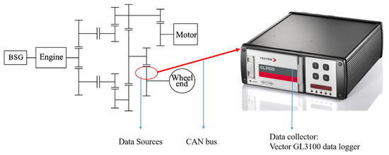
Figure 1.
Test data acquisition equipment.
Considering the typical requirements of vehicles and the national standard “Vehicle Reliability Driving Test Method” (GB/T 12678-90), the typical working conditions included urban roads, provincial roads, expressways, and mountain roads. Due to the large traffic flow on urban roads, the rapid change of road conditions, and more traffic lights, the driving conditions are the most complicated. For urban road conditions, the specific conditions should be fully considered and the selected routes should include expressways, urban trunk roads, and branch roads to ensure that the data are typical. For road conditions other than urban roads, they are less affected by traffic flow, and their operating conditions are relatively stable, so the corresponding test specifications can be used to test to obtain the required load data.
2.2. Statistical Analysis of Load Time History
For plug-in hybrid systems, their working modes are mainly divided into pure electric mode, hybrid mode, engine mode, and kinetic energy recovery mode. When the car starts and drives in medium- and low-speed conditions, it mainly drives in pure electric mode. At this time, the reducer is only subjected to the torque load imposed by the drive motor. When it is necessary to accelerate rapidly or to climb steep slopes, the reducer is subjected to torque load jointly applied by the engine and the drive motor. When the vehicle is in a high-speed cruising state, it is beneficial for the engine to enter a more economical working condition; at this time, the retarder is only subjected to the torque load applied by the engine. When the vehicle is decelerating, the drive motor will absorb part of the power to charge so as to save energy; at this time, the reducer is only subjected to the negative torque applied by the drive motor.
The load time history under the above four working conditions was plotted by MATLAB, and the data were analyzed to check whether the data conformed to the characteristics of typical working conditions. As shown in Figure 2a, when the vehicle speed is lower than 25 km/h, the engine is in a shutdown state and is driven by the drive motor at this time. At this time, the speed of the vehicle is relatively stable, about 20 km/h, but the torque of the motor fluctuates greatly and the vibration frequency is high. After the vehicle speed is greater than 25 km/h, the engine participates in the work and drives the vehicle in conjunction with the drive motor. The torque fluctuation of the engine is smaller than the working fluctuation of the electric motor. When the vehicle speed is in a state of decline, the engine still outputs torque and the torque of the motor is at a negative value. At this time, the motor is in a state of braking recovery. The output of the engine is mainly used to drive the generator to charge the battery, and the engine torque does not pass through the reducer. As shown in Figure 2b, under provincial road conditions, the proportion of the engine torque participating in driving is increased, and the vehicle is driven in hybrid mode most of the time. As shown in Figure 2c, under mountain road conditions, the vehicle is almost exclusively driven in the hybrid mode and the proportion of engine torque is relatively large. Since frequent braking is required when the mountain road goes downhill, it can be found that the negative torque of the drive motor occupies a large proportion. As shown in Figure 2d, under high-speed conditions, the vehicle speed is relatively high and stable, mainly driven by engine torque. The positive torque of the drive motor exists in short-term conditions such as acceleration and overtaking, and the negative torque of the drive motor mainly exists in deceleration. Through comparison of the collected engine and the motor torque load data with the power control strategy, it can be proven that the collected data have good typicality.
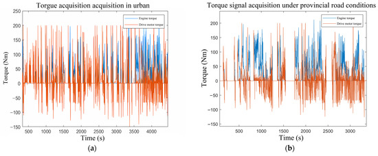
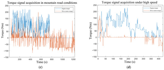
Figure 2.
Load time history diagrams under different working conditions, they are listed as follows: (a) load time history under urban working conditions, (b) load time history under provincial road conditions, (c) load time history under mountain road conditions, and (d) load time history under high-speed conditions.
2.3. Data Preprocessing
2.3.1. Singularity Removal of Load Data
In the process of data acquisition, a small number of singular points are often generated in the data due to the sudden change of equipment current or the influence of the external environment and other factors, which are mainly manifested in a few sampling points, strong randomness, or large values. In this paper, the Signal Process Toolbox in MATLAB was used to remove singular values from the data. In Figure 3, the data from some torque signals are shown. After testing (before processing), there are singular points, such as large values, in the aforementioned figure. After processing, it can be clearly seen that the singular points at the corresponding positions have been removed.
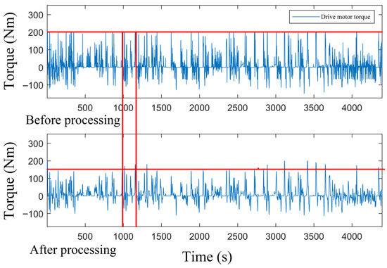
Figure 3.
Comparison diagram of singular point removal of engine torque load data in urban conditions.
2.3.2. Stationarity Test of Load Data
Before performing statistical counting on the measured random load data, it is necessary to ensure that the random load data have stationarity and ergodicity. The usual determination method is to perform a stationarity test and an ergodic test on the random load data. Stationarity includes strict stationarity and wide-sense stationarity. If the joint distribution function of each group of random variables obtained by a random process is time-invariant for different time origins, then the random process is strictly stationary. Wide-sense stationarity is a kind of stationarity that is defined by the characteristic statistics of the series. As long as the low-order moment of the series is guaranteed to be stable, the main properties of the series can be guaranteed to be approximately stable. For a stationary random process, if the statistical mean is equal to the time mean and the statistical autocorrelation function is equal to the time autocorrelation function, it is called the ergodic stationary random process.
The stationary random signals encountered in engineering are generally ergodic, so it is only necessary to perform a stationarity test on the collected random load data. As the stationary digital characteristics of random load data are the mean values and correlation functions of each sample population, it has nothing to do with the value of time. For the convenience of inspection, we decided to adopt the round inspection method for the stationarity test. The basic principle of this method is to divide the random signal into several sub-intervals and calculate the mean square value of the sub-intervals to form a new time series. If the signal is steady state, the change of the new sequence will be random and meet certain statistical laws. Through calculation and consulting the distribution table of the rounds, it can be seen that the collected data have passed the stationarity test.
2.3.3. Determination of Payload Data Invalidity Threshold
Due to the randomness of the vehicle driving conditions, the load on the reducer is a cycle of variable amplitude, and the load cycle has a large difference span. From the measured load data, it can be found that a considerable part of the small-amplitude load exists in the entire load time history. Generally, most small-amplitude loads have little effect on the fatigue life of components, and their occurrence in large numbers can lead to excessively expensive fatigue tests and long test cycles. However, under the action of changing actual loads, small loads will have a non-negligible impact on the fatigue damage of components over time. Therefore, determining an appropriate small load removal standard becomes a necessary condition to ensure the reliability of the load spectrum. For setting the small load removal standard, it can be determined according to
where is the invalid payload threshold, is the maximum value in the random load data, is the minimum value in the random load data, and is the removal rate of the invalid payload. Generally, this value is determined to be 1–10; in this article, it was determined to be 5.
After calculation, the omitted benchmark of invalid amplitude is 16 Nm, that is, the torque value whose absolute value is lower than 16 Nm can ignore the fatigue damage of the reducer. It can be found in Figure 4 that after removing the invalid amplitude, the load time history is reduced from the original 4600 s to only about 1500 s, which is one third of the original load time history. This method retains the effective load data, while the entire load action time is significantly shortened so the load spectrum compiled based on this method can effectively improve the efficiency of the fatigue test.

Figure 4.
The effect diagram of removing the extreme values of invalid load in pure electric mode under provincial road conditions.
2.4. Load Optimal Sample Extraction
2.4.1. Classification of Payload Data
By analyzing the datasets of different working conditions and different modes, it can be found that the operating proportions of the power drive modes of HEV under different working conditions are different. Due to this feature, the output ratio of the drive motor and engine is quite different under different working conditions and the load characteristics (torque mean, standard deviation, and fatigue damage generated) will also be different. Based on this, the collected load time history needs to be further grouped according to the working conditions and power drive modes. A total of 20 sets of data were obtained after processing. Take the following urban conditions as an example: (1) pure electric mode drive motor torque in urban conditions, (2) city engine mode engine torque, (3) hybrid mode drive motor torque in urban conditions, (4) engine torque in hybrid mode in urban conditions, (5) drive motor torque in kinetic energy recovery mode in urban conditions and the corresponding provincial road, highway, and mountain road conditions.
2.4.2. Calculation of Various Criteria for Load Data
In general, the load extreme point and load cycle contain almost all the load information. The mean, standard deviation, and fatigue damage of the load cycle are usually used as the criterion to determine optimal sample length. The mean of the extreme load value can roughly reflect the overall level of the load amplitude, and to a certain extent, it can reflect the influence of the load on the components under various working conditions. The standard deviation of the extreme value of the load can roughly reflect the fluctuation degree of the load amplitude, and to a certain extent, it can reflect the randomness and variation intensity of each working condition. According to the fatigue damage mechanism, the predecessors proposed a method to determine the sample length based on fatigue damage. The calculation formulas of the mean value of the extreme load, the standard deviation of the extreme value of the load, and the fatigue damage of the load cycle are shown in Equations (2)–(4):
Equation (2) is the calculation formula of the mean value of the extreme value of the load. Equation (3) is the formula for calculating the standard deviation of the extreme value of the load. In Equations (2) and (3), is the mean of the extreme loads, is the extreme value, is the number of extreme values, and is the standard deviation of the extreme value of the load.
Equation (4) is the formula for calculating the fatigue damage of load cycles. In Equation (4), is the level of stress at which the sample was collected, is the number of stress cycles at which the sample was collected, and is the corresponding fatigue life of the collected sample.
The fatigue life can be obtained by referring to the S–N curve corresponding to the material at all stress levels. However, since the obtained S–N curve cannot accurately reflect the fatigue life when the number of cycles is small, which directly affects the life estimation accuracy of the reducer gear, it is necessary to correct the S–N curve of the reducer gear to reduce the error of the S–N curve and improve the accuracy of fatigue damage. In this paper, the S–N curve estimation method is used to correct the existing material S–N curve. If the fatigue limit, , and material ultimate strength, , are known, the S–N curve expression is shown as in Equation (5). In the formula, is the stress amplitude of the material, is the number of cycles of failure when the material is subjected to a stress amplitude of , and and are both constants. Its calculation formula is shown in Equations (6) and (7):
For the general fatigue test of metal materials, since the number of cycles is generally large and the fatigue limit is more than 107 time, the error needs to be estimated. Generally, it is assumed that Equation (8) is conservative. In the formula, the coefficients of k are different under different loading modes. When the material is bent, k = 0.5; when the material is subjected to tensile pressure, k = 0.35; and when the material is subjected to torsional deformation, k = 0.29.
The material of the reducer gear studied in this paper is 20 CrMo, its material ultimate strength = 885 MPa, and the coefficient k = 0.5 when subjected to bending. Substitution into Equations (7) and (8) obtained m = 11.75, C = 1245 × 1034, and the studied reducer gear S–N curve. Finally, the value of each criterion under each working condition and each driving mode can be obtained. On the basis of the data obtained in the previous section, the optimal number of samples based on the mean value of the extreme value of the load, the standard deviation of the extreme value of the load, and the fatigue damage of the cyclic fatigue load under each working condition were determined.
The formula for determining the optimal number of samples based on the mean of the extreme value of the load is shown in Equation (9). In the formula, represents the standard deviation of the mean of the extreme values of the sample groups, represents the mean of the extreme values of the groups of samples, and represents the error of the sample. The formula for determining the optimal number of samples based on the standard deviation of load extremes and the formula for determining the optimal number of samples based on cyclic load fatigue damage are shown in Equations (10) and (11), respectively. The symbol in Equation (9) represents the mean value of the standard deviation of the extreme value of the 6 groups of sub-samples. In Equation (11), s represents the standard deviation of the extreme load value, represents the sample mean of the extreme value of the load, represents the percentile of the distribution at the confidence level of , and is the sampling error. The optimal sample number of urban working conditions, as determined according to various criteria, is shown in Table 2.
Table 2.
The optimal number of samples for urban working conditions determined by each criterion.
2.4.3. Optimal Number of Samples Based on a Multi-Criteria Decision-Making Method
The optimal number of samples for each working condition was determined by the multi-criteria decision-making method. Specifically, the weight coefficients corresponding to the three load criteria were obtained by using the subjective weight method and the objective weight method, and the linear weighting method was used to calculate the subjective weight and objective weight. The weighted combination was used to obtain the optimal weight coefficient and finally, the optimal sample length of each working condition was obtained, which provided the optimal sample load for the preparation of the subsequent load spectrum.
This multi-criteria decision-making method adopted three decision-making criteria, namely, the mean value of the extreme load value, the standard deviation of the extreme value of the load, and the fatigue damage of the load cycle. According to the eigenvector method, the subjective weight can be used to obtain the correlation coefficient with a CI ≤ 0.1. It was judged that the relative weight matrix has a good consistency, that is, the subjective relative weight was definitely given. Then, the obtained eigenvectors were normalized to obtain the subjective weight coefficients: .
Using the entropy method to determine the objective weights of the three criteria, the basic idea of this method is as following for different target decisions: the smaller the entropy value of the same criterion, the more obvious the feature it represents is, the greater influence it has on decision making, and the more it should be considered. On the contrary, the larger the entropy value, the less representative the characteristic it represents is, the less influence it has on the decision, and the less it should be considered. This characteristic of the entropy method can pay attention to the load characteristics that should be paid attention to in the process of determining the length of the load sample, which is of great help to the accuracy and rationality of the sample load. The objective weight coefficients of the data of the five working modes are determined according to each criterion, as shown in Table 3.
Table 3.
Objective weight coefficients of the five working mode data.
The optimal weight is determined by the linear combination weighting method, i.e., a weight coefficient is given to the subjective weight and the objective weight, as shown in the following Equation (12). In the formula, is the optimal weight, is the subjective weight, is the objective weight, and and are the linear weight coefficients of subjective weight and objective weight, respectively, that is, the optimal weight coefficient. They need to satisfy . In order to determine the optimal weight coefficient, based on the optimization theory method and the Jaynes maximum entropy method, a mathematical model for determining the weight coefficient is established, and the exact solution of the obtained mathematical model is the optimal weight coefficient. The optimal weight coefficient can be obtained from Equation (13).
According to the formula, and could be obtained as 0.526 and 0.474, respectively. According to Equation (8), the optimal weight coefficient was calculated. The calculation results are shown in Table 4.
Table 4.
Optimal weight coefficients of 5 working mode data.
Through the optimal weight coefficient, the optimal number of samples for each mode under each working condition can be obtained. The maximum optimal sample number across the five power drive modes, the optimal sample number under urban working conditions, was selected. Finally, the optimal sample number can determine the torque load samples of the reducer in each working condition and superimpose them to obtain the final optimal sample of torque loads for multi-condition reducers for load spectrum compilation. One cycle of urban working conditions was 27.5 km, one cycle of provincial road working conditions was 18 km, one cycle of mountain road working conditions was 12 km, and one cycle of high-speed working conditions was 50 km. The optimal multi-condition load corresponds to a mileage of 572 km.
3. Multi-Condition Load Spectrum Compilation and Life Prediction Simulation of Reducer
3.1. Reducer Load Frequency Statistics
Statistical counting of loads is an important part of compiling load spectra, and its principle is to use probability and statistics theory to perform statistical analysis on random loads. In this paper, the rainflow counting method was used for load frequency statistics. The characteristics of the rainflow counting method in the counting process are consistent with the characteristics of the fatigue characteristics of the material. The counting results can truly reflect the fatigue process of the material and have the characteristics of being programmable. The load samples extracted above are counted statistically, wherein the sample loads are divided into positive engine torque, positive torque of the drive motor, and negative torque of the drive motor. Rainflow count statistics are performed for each set of data. The rainflow matrix is shown in Figure 5.
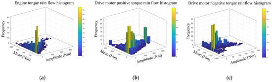
Figure 5.
Torque rain flow matrix of each power source under urban conditions: (a) engine torque rainflow matrix, (b) drive motor positive torque rainflow matrix, (c) drive motor negative torque rainflow matrix.
3.2. Reducer Load Spectrum Extrapolation
In view of the limitation of test time, cost, and other factors, it is often impossible to collect the actual load spectrum of a component throughout its life cycle. This problem can be effectively solved by using load spectrum extrapolation. Its basic idea is as follows: By collecting the load-time history of a limited time as a sample, using the sample as the basis of the full-life load-time history of the component, and using reasonable extrapolation technology to extrapolate the sample load, it is possible to obtain the possible occurrence of the component in the entire life cycle. Finally, the magnitude and frequency of the load that may occur within the entire life cycle of the component can be obtained.
Since the rainflow counting method itself has the characteristic that its load counting results are consistent with the fatigue hysteresis loop, in order to ensure that this characteristic is not destroyed in the extrapolation process, the rainflow matrix nonparametric extrapolation method is selected in this paper to extrapolate the load spectrum. Compared with the parametric estimation method, the non-parametric estimation method does not rely on assumptions about the distribution of the load mean and amplitude and does not cut off the connection between the load mean and amplitude. The influence of subjective factors in the process of assuming distribution type is avoided as much as possible. The results of the non-parametric estimation method are completely determined by the test sample data, which is more objective, so that the extrapolated load spectrum can be more representative of the actual working conditions. In this paper, the Epanechnikov kernel function was selected for nonparametric density estimation. Compared to the Gaussian kernel function, its calculation is simple and there is no restriction on the concentration direction of the sample data, which is more suitable for the extrapolation of the load spectrum. The kernel function generally selects the Gaussian kernel density function and the Epanechnikov kernel function, and their expressions are shown in Equations (14) and (15):
In this study, four road conditions were selected to collect the torque loads on the reducer, namely: urban conditions, high-speed conditions, provincial road conditions, and mountain road conditions. It is necessary to allocate the cumulative frequency of the reducer’s life cycle according to the proportion of the four actual working conditions. It can be seen that the proportion of road conditions actually used by ordinary users is:
(Highway): (City): (Provincial Road): (Mountain Road) = 50:30:15:5.
From the proportions of the four typical road conditions and the sum of the cumulative frequency of loads under the five power drive modes under a single road condition, the cycle times of each extrapolated condition can be calculated according to Equation (16). In the formula, is the cumulative frequency allocated by the ith working condition in the whole life cycle; is the limit number of load cycles, which is usually taken as 106 in engineering; and is the proportion of the ith working condition. After obtaining the cycle times of each working condition after the extrapolation, the extrapolation coefficient of the rainflow matrix under the corresponding working condition was calculated according to Equation (17). In the formula, is the extrapolation coefficient of the rainflow matrix of the ith working condition and is the cumulative frequency of the jth working section in the ith working condition.
The total frequency of the effective load of the four working conditions collected from the actual road load is 692 times in the city, 2089 times in the provincial road condition, 601 times in the mountain road condition, and 592 times in the high-speed working condition. From Equations (16) and (17), the extrapolation coefficients of the rainflow matrix for the four road conditions were obtained as = 434, = 72, = 84, = 846. Among them, the sample sizes of engine torque for four road conditions were = 96, = 997, = 221, and = 375, and the corresponding standard deviation was 399.79. The sample sizes of the positive torque of the drive motor for the four road conditions were = 356, = 496, = 101, and = 57, and the corresponding standard deviation was 209.11. The sample sizes of the negative torque of the drive motor for the four road conditions were = 241, = 596, = 279, = 160, and the corresponding standard deviation is 191.22.
According to the extrapolation coefficient of each working condition, the extrapolation method of non-parametric kernel density estimation was applied, the rainflow matrix was extrapolated with the help of a software data processing module, and the extrapolated rainflow matrix with different torque loading modes under different working conditions was obtained. The extrapolated rainflow matrix is shown in Figure 6. It can be seen that the frequency of the extrapolated rainflow matrix was increased from dozens of times before the extrapolation to tens of thousands of times, and the extrapolation effect is obvious.
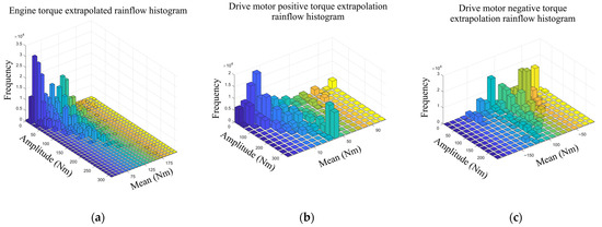
Figure 6.
Torque extrapolation rain flow matrix of each power source under urban working conditions: (a) engine torque extrapolation rainflow matrix, (b) drive motor positive torque rainflow matrix, (c) drive motor negative torque rainflow matrix.
3.3. Program Load Spectrum Compilation and Simulation Application
3.3.1. Synthesis and Dimensionality Reduction of Load Spectrum
The extrapolated load spectrum of each working condition was classified and superimposed according to the action mode of the power source, and the extrapolated load spectrum of the engine torque, the positive torque of the driving motor, and the negative torque of the driving motor under all working conditions was obtained. When superimposing the two-dimensional load spectrum, it is necessary to ensure that the matrix scale of the two-dimensional load spectrum is consistent. Here, the two-dimensional load spectrum was edited. First, the two-dimensional load spectrum of the same torque loading mode is converted to the same scale, and then the two-dimensional load spectrum of the same torque loading mode under each working condition was superimposed. In order to facilitate the subsequent compilation of the program load spectrum suitable for the bench, the synthesized two-dimensional load spectrum needs to be of the “amplitude-mean” type.
The two-dimensional load spectrum of the rainflow counting is more realistic to the simulation of the actual load information of the reducer, but the two-dimensional load spectrum is difficult to load on the bench. Therefore, it is necessary to convert the two-dimensional load spectrum into a one-dimensional load spectrum that can be used for bench tests. In this paper, the fluctuation center method was used, that is, a variable amplitude load was applied on the basis of a certain mean value to realize the dimensionality reduction of the two-dimensional load spectrum. In this paper, Equation (18) was used to obtain the amplitude load based on a certain mean value, that is, the sum of the products of the mean value of each load in the two-dimensional rainflow spectrum and its corresponding cumulative frequency is divided by the total frequency of the load contained in this rainflow matrix. is the fluctuation center, is the mean value of loads at all levels, is the frequency corresponding to the mean values of loads at all levels, and is the total frequency of loads included in the rainflow matrix. Due to the large amount of one-dimensional load spectrum data, Table 5 only shows the one-dimensional load spectrum of the positive torque of some drive motors.
Table 5.
One-dimensional load spectrum of drive motor positive torque (part).
3.3.2. Program Load Spectrum Compilation
The one-dimensional load spectrum is classified according to the amplitude. Currently, the most widely-used classification method is eight-level classification, i.e., according to the maximum value of the entire load section multiplied by the proportional coefficient: 1, 0.95, 0.85, 0.725, 0.575, 0.425, 0.275, and 0.125. All load values are grouped into these eight amplitudes, resulting in eight amplitude levels. Using the equal damage conversion principle, the continuous cumulative frequency curve extrapolated from the rainflow matrix is converted into an eight-level program load spectrum. Compared with the fixed-amplitude load spectrum, the eight-level program load spectrum has the ability to reproduce the loads that the components are subjected to under the actual working conditions.
Since the rainflow counting method was used in the initial stage of load compilation, the loading sequence of the load cycle was not considered, so the influence of the amplitude loading sequence on the fatigue endurance test should be considered when compiling the bench loading spectrum. At present, the “low-high-low” loading method is mainly used to solve this problem. The transformed program load spectrum block is shown in Figure 7. The above eight-level program load spectra with different torque loading methods are sequentially combined into a complete multi-condition program load spectrum 48. During the bench test, the load simulation of the reducer under multiple working conditions can be realized by simply loading the program load spectrum blocks in sequence.

Figure 7.
Program load spectrum block of each driving mode under full operating conditions: (a) engine torque program load spectrum block, (b) drive motor positive torque program load spectrum block, (c) drive motor negative torque program load spectrum block.
3.4. Fatigue Life Prediction Simulation of Reducer Gears
The prepared programmed load spectrum was used as the load input, the fatigue life of the reducer was predicted by finite element simulation, the fatigue life of the reducer was compared with the actual sample load as the load input, and the validity of the programmed load spectrum is finally verified. The reducer gear must be 3D-modeled prior to finite element analysis. In this paper, the three-dimensional modeling software Creo was used for parametric modeling of helical gears. The remaining size parameters were obtained by the formula to realize the rapid establishment of the gear model.
The finite element analysis software (ANSYS Workbench) was used to carry out finite element simulation analysis of gear fatigue life. The 3D model of the helical gear built in Creo was imported into the Workbench and the material parameters of the helical gear (including elastic model, density, Poisson’s ratio, etc.) were set. Considering the slippage during the meshing process of the helical gear, the contact type was selected as “Frictional”, and the friction coefficient was 0.1. Considering that the pair of helical gears were all swept bodies, the mesh setting of the helical gear pair was performed, and the meshing of the helical gear pair was realized by swept hexahedral mesh, so as to obtain the finite element model of the helical gear pair. The element index of most of the grids in this paper was 0.8–0.9, and the grid quality met the requirements.
In this paper, translation constraints, rotational constraints, and torque loads were mainly applied to the helical gear. For the driving wheel, the translation in the three directions of X, Y, and Z, and the rotation in the two directions of the X and Y axes (a total of 5 degrees of freedom) were constraining, only releasing the degree of freedom of rotation around the Z axis, while applying a moment on the inner ring to rotate around its axis. For the driven wheel, the above six degrees of freedom were constrained without any load. The stress value of the solution result was 1177 MPa, and the gear stress was mainly concentrated in the root of the tooth, as the root of the tooth is most likely to break. This phenomenon is basically consistent with the actual gear failure phenomenon, which verifies the reliability of the gear model and the static finite element analysis. The solution results were used for subsequent gear fatigue life prediction. The fatigue simulation analysis in this paper mainly selected the nCode DesignLife module in ANSYS Workbench. The load spectrum file that has been prepared above was imported in the “TimeSeries Input” module, and the fatigue life distribution cloud diagram of the reducer helical gear, as shown in Figure 8, was obtained.
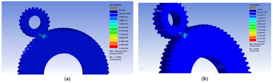
Figure 8.
Simulation analysis results of gear fatigue life prediction: (a) fatigue life simulation of gears based on program load spectrum and (b) fatigue life simulation of gears based on actual loads.
It can be seen in Figure 8 that the parts prone to fatigue damage on the gear are mainly concentrated at the root of the tooth, which is consistent with the static stress analysis results and the actual reducer gear bench durability test results. At the same time, it was found that when the program load spectrum was used as the input, the fatigue life of the reducer gear was 1.412 × 10³, i.e., the reducer gear was loaded with 1.412 × 10³ cycles of fatigue damage in the program load spectrum, which is equivalent to 807,000 kilometers of driving the car, and the reducer gear was damaged. When the actual load was used as the input load, the fatigue life of the reducer gear was 1.933 × 10³, i.e., the reducer gear was fatigued after the actual load was applied for 1.933 × 10³ cycles, which is equivalent to 1.103 million kilometers of driving the car, and failure occurred. Comparing the reducer gear fatigue life of the programmed load spectrum with the actual load reducer gear fatigue life, the relative error was 26%, which is within the normal range, and the validity of the programmed load spectrum can be verified.
4. Conclusions
Aimed at alleviating the problem of the lack of load spectra suitable for hybrid electric vehicles, research on the compilation method of hybrid electric vehicle load spectra is carried out mainly in three aspects: load data acquisition, load data processing, and load data statistical counting and extrapolation of fatigue life prediction of reducer gears in hybrid electric vehicles.
Based on the roads in Shenzhen, typical working condition routes were selected for the real vehicle data collection test, including urban working conditions, provincial road working conditions, mountain road working conditions, and high-speed working conditions. Whether the collected load data had the characteristics of typical working conditions was analyzed. Considering that the influence of the fatigue life of the reducer under the action of the engine and the action of the drive motor is quite different, the load data under each typical working condition were divided into five categories according to the power source state. The classified data were processed by singular value removal, invalid amplitude removal, and stationarity testing. The optimal number of samples with the load extreme mean value, the load extreme standard deviation, and the cyclic load fatigue damage as the criteria were calculated. The subjective weighting method and the objective weighting method were used to determine the subjective weighting coefficient and the objective weighting coefficient under each criterion, respectively, and the optimal weighting coefficient under each criterion was obtained by the linear weighting method. Then, the samples under each working condition were weighted to obtain the optimal number of samples for each working condition, and the optimal sample load for compiling the load spectrum was obtained.
Rainflow counting and non-parametric extrapolation based on rainflow matrix are carried out on three types of data divided according to the power source output to obtain the full-life two-dimensional load spectrum of the hybrid electric vehicle reducer and the fluctuation center method was used to convert the two-dimensional load spectrum. Dimensionality reduction to obtain a one-dimensional load spectrum was performed. The cumulative frequency of the load was divided into eight levels based on the load amplitude, and the full-life eight-level program load spectrum that can be used for the bench test was obtained. Finally, as determined by the fatigue life simulation, the relative error was 26% when comparing the fatigue life results of the reducer whose load input was the optimal sample load. This shows that the programmed load spectrum has the ability to represent the actual load situation, which verifies the validity of the programmed load spectrum.
In the future, the data collection can be improved. Due to the differences in the driving styles of different drivers, there will be some differences in the load spectrum data collected on the same road section, so more drivers can be allowed to conduct more tests on various road conditions in the future. This can improve the accuracy and universality of the compiled load spectrum. In addition, the load spectrum compilation method for hybrid electric vehicles proposed in this paper is also applicable to other regions. The load spectra of hybrid electric vehicles in various regions can be compiled to form a load spectrum database, which is very meaningful.
Author Contributions
Conceptualization, J.L. and W.W.; methodology, C.H.; software, T.T.; validation, X.R. and Z.Z.; formal analysis, S.S.; investigation, J.L.; resources, W.W.; data curation, writing—original draft preparation, J.L.; writing—review and editing, J.L.; project administration and Supervision, W.W.; funding acquisition, C.H. All authors have read and agreed to the published version of the manuscript.
Funding
This research was funded by R&D Program in Key Fields of Guangdong Province—R&D and Application of Key Technologies for New Energy Vehicle Gearboxes with High Efficiency, High Precision, Long Life and Low Noise (2020B090926004), Guangdong Province Key Field R&D Program—Electric Vehicle Powertrain Design and Optimization Industrial Software (2021B0101220003), Guangdong Laboratory for Lingnan Modern Agriculture Project (NT2021009).
Institutional Review Board Statement
Not applicable.
Informed Consent Statement
Not applicable.
Data Availability Statement
Not applicable.
Conflicts of Interest
The authors declare no conflict of interest.
References
- Yu, P.; Zhang, J.; Yang, D.; Lin, X.; Xu, T. The Evolution of China’s New Energy Vehicle Industry from the Perspective of a Technology–Market–Policy Framework. Sustainability 2019, 11, 1711. [Google Scholar] [CrossRef] [Green Version]
- Carley, S.; Krause, R.M.; Lane, B.W.; Graham, J.D. Intent to purchase a plug-in electric vehicle: A survey of early impressions in large US cites. Transp. Res. D Transp. Environ. 2013, 18, 39–45. [Google Scholar] [CrossRef]
- Xu, X.; Chen, X.; Liu, Z.; Yang, J.; Xu, Y.; Zhang, Y.; Gao, Y. Multi-objective reliability-based design optimization for the reducer housing of electric vehicles. Eng. Optim. 2021, 2021, 1–17. [Google Scholar] [CrossRef]
- Zeng, Y.; Huang, Z.; Cai, Y.; Liu, Y.; Xiao, Y.; Shang, Y. A Control Strategy for Driving Mode Switches of Plug-in Hybrid Electric Vehicles. Sustainability 2018, 10, 4237. [Google Scholar] [CrossRef] [Green Version]
- Guercioni, G.R.; Vigliani, A. Gearshift control strategies for hybrid electric vehicles: A comparison of powertrains equipped with automated manual transmissions and dual-clutch transmissions. Proc. Inst. Mech. Eng. Part D 2019, 233, 2761–2779. [Google Scholar] [CrossRef]
- Lin, C.H. Modeling and analysis of power trains for hybrid electric vehicles. Int. Trans. Electr. Energ. Syst. 2018, 28, e2541. [Google Scholar] [CrossRef]
- Liu, X.; Zheng, S.; Chen, T.; Liang, G.; Feng, J.; Ning, X. Durability Testing Method of a Hub-Reducer System Based on the Shanghai Standard Road Driving Cycle. J. Test. Eval. 2016, 44, 665–678. [Google Scholar] [CrossRef]
- Chłopek, Z.; Lasocki, J.; Wójcik, P.; Badyda, A.J. Experimental investigation and comparison of energy consumption of electric and conventional vehicles due to the driving pattern. Int. J. Green Energy 2018, 15, 773–779. [Google Scholar] [CrossRef]
- Cai, Y.; Dou, L.; Hu, D.; Chen, L.; Shi, D.; Wang, J. Torque distribution method based on vibration instability of PS-HEV transmission system. Proc. Inst. Mech. Eng. Part D 2020, 234, 3491–3503. [Google Scholar] [CrossRef]
- Oh, S.C.; Emadi, A. Test and simulation of axial flux-motor characteristics for hybrid electric vehicles. IEEE Trans. Veh. Technol. 2004, 53, 912–919. [Google Scholar] [CrossRef]
- Liu, Z.K.; Peng, C.; Yang, X.Q. Research and analysis of the wheeled vehicle load spectrum editing method based on short-time Fourier transform. Proc. Inst. Mech. Eng. Part D J. Automot. Eng. 2019, 233, 3671–3683. [Google Scholar] [CrossRef]
- Zheng, G.F.; Wang, Q.Y.; Cai, C. Criterion to determine the minimum sample size for load spectrum measurement and statistical extrapolation. Measurement 2021, 178, 109387. [Google Scholar] [CrossRef]
- Su, H. A Road Load Data Processing Technique for Durability Optimization of Automotive Products. SAE Int. J. Passeng. Cars Mech. Syst. 2014, 7, 244–259. [Google Scholar] [CrossRef]
- Shen, Y.F.; Zheng, S.L.; Wang, Z.R.; Liang, G.Q.; Ma, Z.G. Complication on the Spectrum of Automotive Swing Arm Due to Low-Amplitude Loads. Int. J. Automot. Technol. 2015, 16, 447–455. [Google Scholar] [CrossRef]
- Gao, Y.F.; Zhang, X.F.; Xue, J.F.; Liu, H. Study on load spectrum of gear program based on rain flow counting method. Mach. Tool Hydraul. 2020, 48, 11–15. [Google Scholar]
- Wang, J.X.; Ji, J.F.; Zhang, Y.S.; Wang, N.X.; Zhang, E.P.; Huang, J.J. Noise Reduction Method for Time Domain Load Signal of Engineering Vehicles Based on Wavelet Fractal Theory. J. Jilin Univ. Eng. Sci. 2011, 41, 221–225. [Google Scholar]
- Gong, H.B.; Su, J.; Wang, X.Y.; Xu, G.; Zhang, Y.R. Load spectrum compilation of high-speed train gear transmission based on extreme value extrapolation. J. Jilin Univ. 2014, 5, 1264–1269. [Google Scholar]
- Jia, P.; Liu, H.; Zhu, C. Contact fatigue life prediction of a bevel gear under spectrum loading. Front. Mech. Eng. 2020, 15, 123–132. [Google Scholar] [CrossRef] [Green Version]
- Pham, Q.H.; Gagnon, M.; Antoni, J.; Tahan, A.; Monette, C. Rainflow-counting matrix interpolation over different operating conditions for hydroelectric turbine fatigue assessment. Renew. Energ. 2021, 172, 465–476. [Google Scholar] [CrossRef]
- Cui, C.; Chen, A.; Ma, R.; Wang, B.; Xu, S. Fatigue Life Estimation for Suspenders of a Three-Pylon Suspension Bridge Based on Vehicle-Bridge-Interaction Analysis. Materials 2019, 12, 2617. [Google Scholar] [CrossRef] [Green Version]
- Fu, B.; Zhao, J.; Li, B.; Yao, J.; Teifouet, A.R.M.; Sun, L.; Wang, Z. Fatigue reliability analysis of wind turbine tower under random wind load. Struct. Saf. 2020, 87, 101982. [Google Scholar] [CrossRef]
- Wang, M.-L.; Liu, X.-T.; Wang, X.-L.; Wang, Y.-S. Research on Load-Spectrum Construction of Automobile Key Parts Based on Monte Carlo Sampling. J. Test. Eval. 2018, 46, 1099–1110. [Google Scholar] [CrossRef]
- Yang, Z.; Song, Z.; Zhao, X.; Zhou, X. Time-domain extrapolation method for tractor drive shaft loads in stationary operating conditions. Biosyst. Eng. 2021, 210, 143–155. [Google Scholar] [CrossRef]
- Ma, S.; Sun, S.; Wang, B.; Wang, N. Estimating load spectra probability distributions of train bogie frames by the diffusion-based kernel density method. Int. J. Fatigue 2020, 132, 105352. [Google Scholar] [CrossRef]
- Aggarwal, M. Decision aiding model with entropy-based subjective utility. Inf. Sci. 2019, 501, 558–572. [Google Scholar] [CrossRef]
- Wang, J.; Hu, J.; Yao, M.; Wang, Z. Estimating load spectra probability distributions of train bogie frames by the diffusion-based kernel density method. Proc. Inst. Mech. Eng. Part C 2012, 226, 1148–1161. [Google Scholar] [CrossRef]
- Yang, X.B.; Liu, X.T.; Tong, J.C.; Wang, Y.S.; Wang, X.L. Research on Load Spectrum Construction of Bench Test Based on Automotive Proving Ground. J. Test. Eval. 2018, 46, 20170201. [Google Scholar] [CrossRef]
- Curtis Berthelot, P.E.; Podborochynski, D.; Brent Marjerison, P.E.; Ron Gerbrandt, P.E. Saskatchewan Field Case Study of Triaxial Frequency Sweep Characterization to Predict Failure of a Granular Base across Increasing Fines Content and Traffic Speed Applications. J. Transp. Eng. 2009, 135, 907–914. [Google Scholar] [CrossRef]
- Angelo, C.M.; Machado, F.A.C.; Schön, C.G. Influence of tire sizes over automobile body spectrum loads and fatigue damage accumulation. Mater. Des. 2015, 67, 385–389. [Google Scholar] [CrossRef]
- Xu, L.; Dai, G.Z. Accelerated Life Test and FEM Simulation-Based Fatigue Analysis of an Aluminum Alloy Push Rod. Scr. Mater. 2019, 51, 32–39. [Google Scholar] [CrossRef]
- Wang, S.; Liu, X.; Jiang, C.; Wang, X.; Wang, X. Prediction and evaluation of fatigue life for mechanical components considering anelasticity-based load spectrum. Fatigue Fract. Eng. Mater. Struct. 2021, 44, 129–140. [Google Scholar] [CrossRef]
- Dong, Q.; Yu, Y.; Xu, G. Fatigue residual life estimation of jib structure based on improved v-SVR algorithm obtaining equivalent load spectrum. Fatigue Fract. Eng. Mater. Struct. 2020, 43, 1083–1099. [Google Scholar] [CrossRef]
- Lei, X.U.; Cao, H.; Liu, H.; Zhang, Y. Assessment of fatigue life of remanufactured impeller based on FEA. Front. Mech. Eng. 2016, 11, 219–226. [Google Scholar]
- Wu, Y.; Xu, Y.; Guo, X.; Bao, R. Fatigue life prediction based on equivalent initial flaw size for Al-Li alloy 2297 under spectrum loading. Int. J. Fatigue 2017, 103, 39–47. [Google Scholar] [CrossRef]
- Luo, J.; Wang, S.; Liu, X.; Geng, S. Fatigue life prediction of train wheel shaft based on load spectrum characteristics. Adv. Mech. Eng. 2021, 13, 1–10. [Google Scholar] [CrossRef]
- Ye, N.H.; He, Y.; Deng, X.; Cheng, C.C. An improved damage model using the construction technology of virtual load spectrum and its statistical analysis. Fatigue Fract. Eng. Mater. Struct. 2018, 41, 1706–1716. [Google Scholar] [CrossRef]
- Wang, H.; Xuan, F.; Liu, X. Prediction and evaluation of fatigue life under random load based on low load strengthening characteristic. Int. J. Fatigue 2021, 151, 106346. [Google Scholar] [CrossRef]
- Li, J.; Zhang, X.; Li, J.; Liu, Y.; Wang, J. Building and optimization of 3D semantic map based on Lidar and camera fusion. Neurocomputing 2020, 409, 394–407. [Google Scholar] [CrossRef]
- Yang, C.; Huang, D.; He, W.; Cheng, L. Neural control of robot manipu-lators with trajectory tracking constraints and input saturation. IEEE Trans. Neural Netw. Learn. Syst. 2020, 32, 4231–4242. [Google Scholar] [CrossRef]
Publisher’s Note: MDPI stays neutral with regard to jurisdictional claims in published maps and institutional affiliations. |
© 2022 by the authors. Licensee MDPI, Basel, Switzerland. This article is an open access article distributed under the terms and conditions of the Creative Commons Attribution (CC BY) license (https://creativecommons.org/licenses/by/4.0/).