
Unlocking the Flexibility of District Heating Pipeline Energy Storage with Reinforcement Learning


Abstract
:1. Introduction
- Environment uncertainty
- Modeling uncertainty
- Scarcity of placed sensors
1.1. Related Work
1.2. Main Contributions
- Modeling of CHP economic dispatch with DHN pipeline storage as a Markov decision process:
- -
- The construction and performance comparison of the RL with a full state space and a partial state space created from the realistically available sensory information.
- -
- The creation of the reward function incorporating a system’s limitations and safety guarantees.
- The RL approach is compared with an exhaustive mathematical optimizer [12] on a half-year dataset for trading on the day-ahead and real-time electricity market, and it showed better stability guarantees, higher feasibility when evaluated with the simulator, and time scale flexibility, while making moderate profit gain for shorter pipes.
2. Mathematical Modeling and Optimization of the District Heating System
2.1. Mathematical Model of the District Heating System
2.2. Solving the Mathematical Model
2.3. Model of a Profit Upper Bound
2.4. Model of a Basic Control Strategy
3. Formulation of a Reinforcement Learning Framework for the District Heating System Control
3.1. Action Space
3.2. State Space
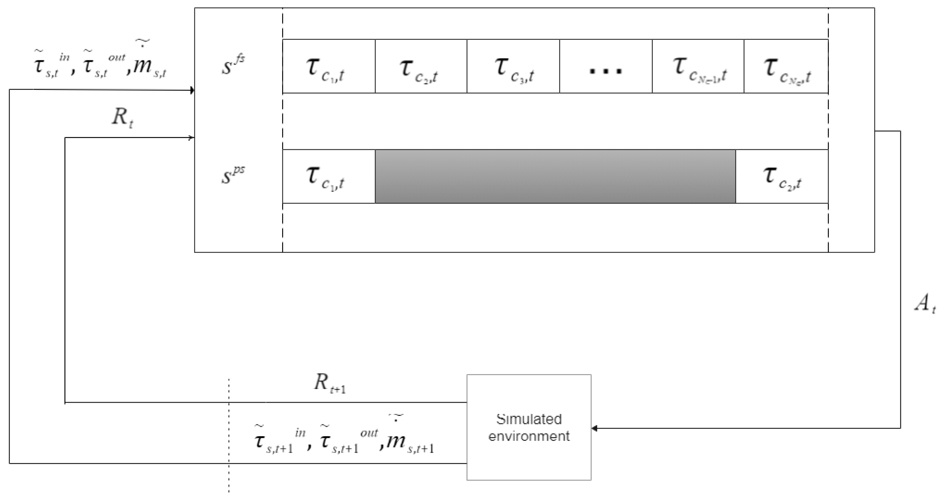
3.2.1. Full State Space
3.2.2. Partial State Space
3.3. Reward Engineering
3.3.1. Profit Sub-Reward
3.3.2. Underdelivered Heat Sub-Reward
3.3.3. Minimal and Maximal Temperature Sub-Reward
3.3.4. Maximal Mass Flow Sub-Reward
4. Experimental Design
5. Overview of the Simulator
6. Experimental Results on Two Case Studies
6.1. Full versus Partial State Space Q-Learning
6.2. Full State Space Q-learning versus Mixed-Integer Nonlinear Program

6.2.1. Performance
6.2.2. Stability

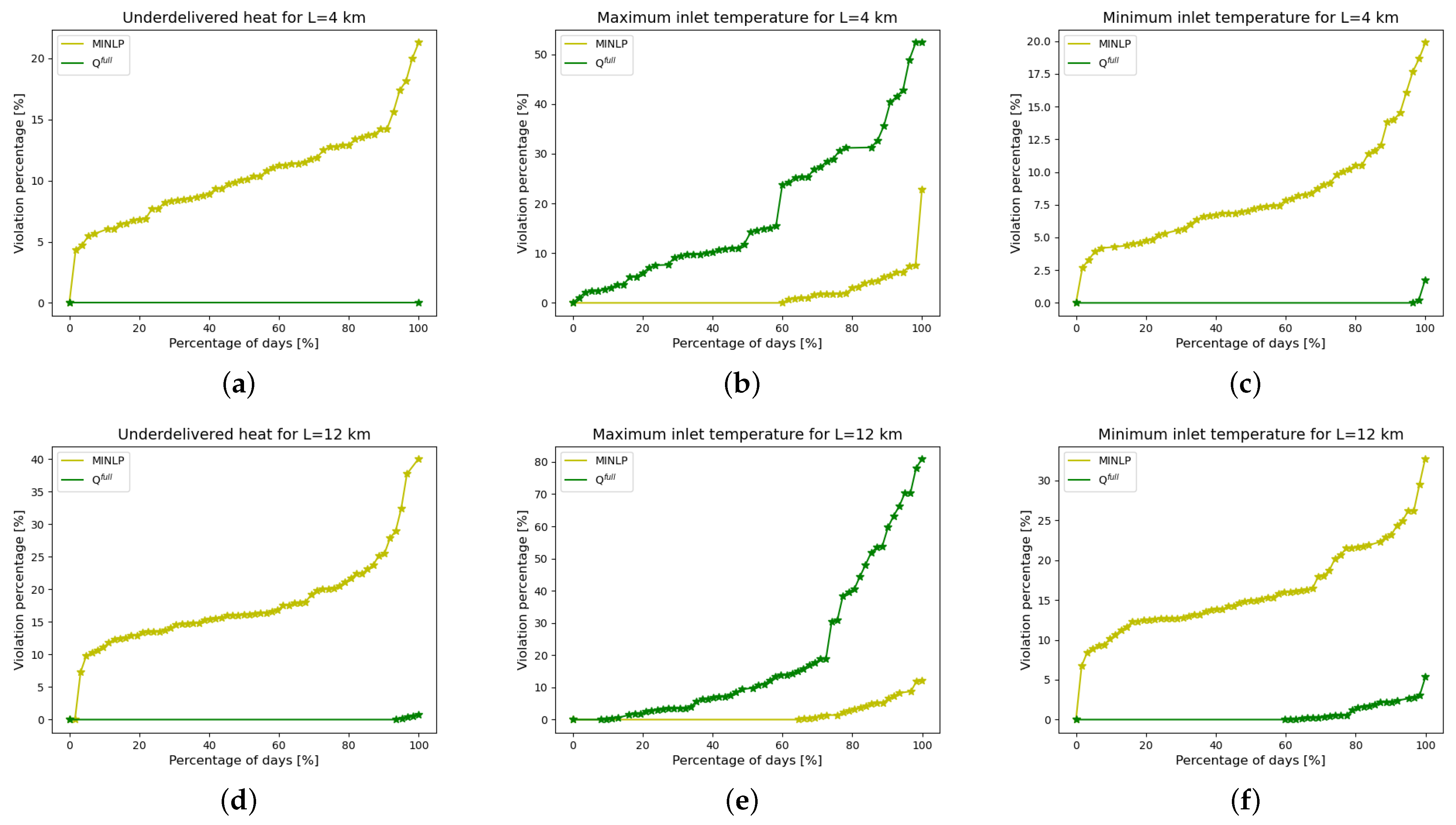
6.2.3. Feasibility
6.2.4. Time-Scale Flexibility
7. Conclusions
Author Contributions
Funding
Institutional Review Board Statement
Informed Consent Statement
Data Availability Statement
Conflicts of Interest
Nomenclature
| Maximum mass flow. | |
| Mass flow at the time-step t characterizing partial state space of a Q-learning | |
| algorithm — equal to the mass flow of the simulation environment . | |
| Mass flow in the supply network at the time-step t. | |
| Upper bound on profit at the time-step t. | |
| Upper bound on sub-reward functions concerning temperature (Hyperparameter of | |
| a Q-learning algorithm). | |
| Upper bound on underdelivered heat sub-reward function (Hyperparameter of | |
| a Q-learning algorithm). | |
| Upper bound on profit sub-reward function (Hyperparameter of a Q-learning | |
| algorithm). | |
| Upper bound on maximum mass flow sub-reward (Hyperparameter of a Q-learning | |
| algorithm). | |
| Lower bound on sub-reward functions concerning temperature (Hyperparameter of | |
| a Q-learning algorithm). | |
| Lower bound on underdelivered heat sub-reward function (Hyperparameter of | |
| a Q-learning algorithm). | |
| Lower bound on profit sub-reward function (Hyperparameter of a Q-learning | |
| algorithm). | |
| Lower bound on maximum mass flow sub-reward (Hyperparameter of a Q-learning | |
| algorithm). | |
| Mass flow in the supply network at the time-step t of the simulation environment. | |
| Mass flow in the supply network of the secondary side grid at the time-step t of the | |
| simulation environment. | |
| Delivered heat to the consumer at the time-step t of the simulation environment. | |
| A | Set of actions of Q-learning algorithm. |
| Cost coefficient of the heat production. | |
| Cost coefficient of the electricity production. | |
| Surface area of the pipe walls. | |
| Surface area of the pipe. | |
| Action of a Q-learning agent at the time-step t (belongs to the set of actions A). | |
| C | Heat capacity of the water. |
| Maximum electricity price. | |
| Minimum electricity price. | |
| Price of the electricity at the time-step t. | |
| F | Profit function over the optimization horizon T. |
| Profit function at the time-step t. | |
| Cumulative reward at the time-step t. | |
| h | Thermal resistance. |
| Delivered heat to the consumer at the time-step t. | |
| Maximal delivered heat to the consumer. | |
| Minimal delivered heat to the consumer. | |
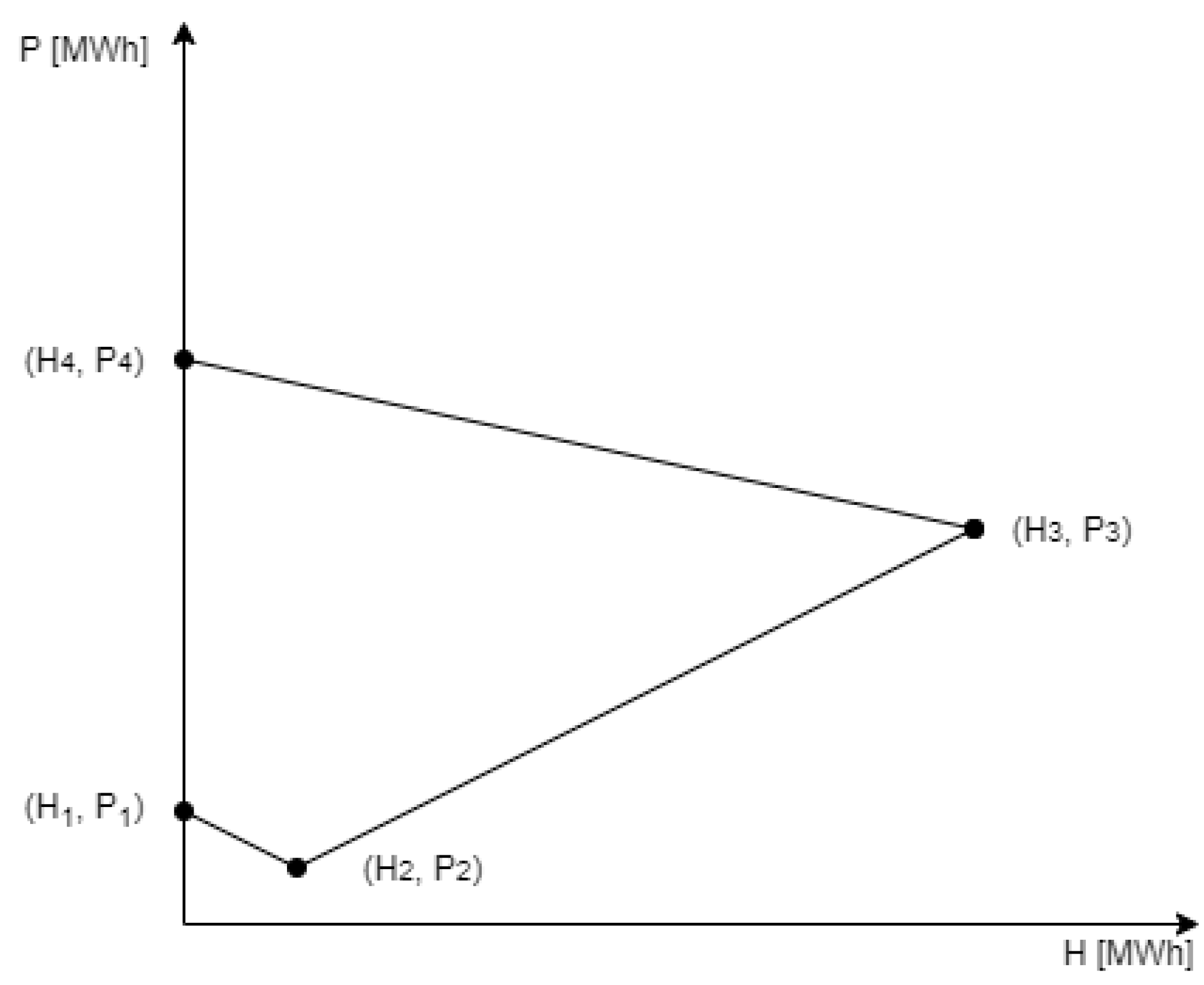
| Heat corresponding to the ith characteristic point of the CHP operating region. | |
| Produced heat at the time-step t. | |
| L | Length of the pipe. |
| Mass of the ith water chunk at the time-step t. | |
| Number of temperature points in a Q-learning state space. | |
| Number of action points of Q-learning algorithm. | |
| Number of water chunks. | |
| Number of water chunks of the same temperature. | |
| Set of characteristic points of the CHP unit. | |
| O | Set of observations of a Q-learning algorithm. |
| Observation provided by a simulation environment at the time-step t (belongs to the | |
| set of observations O). | |
| P | The probability of the transition (at the time-step t) to the state from the state |
| under action . | |
| Electricity corresponding to the ith characteristic point of the CHP operating region. | |
| Produced electricity at the time-step t. | |
| Minimal heat load pressure at the heat exchange station. | |
| Q-value of executing action at the state . | |
| A full state space of a Q-learning algorithm. | |
| Maximum heat demand. | |
| Minimum heat demand. | |
| A partial state space of a Q-learning algorithm. | |
| Consumer’s heat demand at the time-step t. | |
| R | Set of reward functions of Q-learning algorithm. |
| Maximum value of profit sub-reward function. | |
| Minimum value of profit sub-reward function. | |
| Reward provided by a simulation environment at the time-step t (belongs to the set | |
| of rewards R). | |
| Profit sub-reward function of a Q-learning algorithm at the time-step t. | |
| Underdelivered sub-reward function of a Q-learning algorithm at the time-step t. | |
| Maximum mass flow sub-reward function of a Q-learning algorithm at the | |
| time-step t. | |
| Maximum supply network inlet temperature sub-reward function of a Q-learning | |
| algorithm at the time-step t. | |
| Minimum return network inlet temperature sub-reward function of a Q-learning | |
| algorithm at the time-step t. |
| Minimum supply network inlet temperature sub-reward function of a Q-learning | |
| algorithm at the time-step t. | |
| S | Set of states of Q-learning algorithm. |
| State of an environment of a Q-learning algorithm at the time-step t (belongs to the | |
| set of states S). | |
| External state space of a Q-learning algorithm at the time-step t. | |
| Internal state space of a Q-learning algorithm at the time-step t. | |
| Internal part of a Q-learning full state space at the time-step t. | |
| Internal part of a Q-learning partial state space at the time-step t. | |
| Season at the time-step t—part of the state of a Q-learning algorithm. | |
| Time of the day at the time-step t—part of the state of a Q-learning algorithm. | |
| T | Optimization horizon. |
| Greek symbols | |
| Learning rate of a Q-learning algorithm. | |
| Variable representing the ith characteristic point of the CHP operating region at the | |
| time-step t. | |
| Maximum mass flow violation. | |
| Minimum mass flow violation. | |
| Mass flow discretization step. | |
| Temperature discretization step. | |
| Maximum temperature violation. | |
| Minimum temperature violation. | |
| Mass discretization step. | |
| Optimization interval | |
| Exploration–exploitation parameter of a Q-learning algorithm. | |
| Future rewards discount of a Q-learning algorithm. | |
| Density of the water. | |
| Temperature of the environment. | |
| Temperature of the ith water chunk at the time-step t. | |
| Temperature at the inlet of the return network at the time-step t. | |
| Temperature at the outlet of the return network at the time-step t. | |
| Minimum temperature at the inlet of the return network. | |
| Temperature at the outlet of the supply network at the time-step t. | |
| Temperature at the inlet of the supply network at the time-step t. | |
| Maximum temperature at the inlet of the supply network. | |
| Minimum temperature at the inlet of the supply network. | |
| Temperature at the outlet of the return network of the secondary side grid at the | |
| time-step t of the simulation environment. | |
| Temperature at the inlet of the supply network of the secondary side grid at the | |
| time-step t of the simulation environment. | |
| Temperature at the inlet of the supply network at the time-step t of the | |
| simulation environment. | |
| Temperature at the outlet of the supply network of the secondary side grid at the | |
| time-step t of the simulation environment. | |
| Temperature at the outlet of the supply network at the time-step t of the | |
| simulation environment. | |
| Gradient of a temperature sub-reward function (Hyperparameter of a Q-learning | |
| algorithm). | |
| Gradient of a heat sub-reward function (Hyperparameter of a Q-learning algorithm). | |
| Gradient of a mass flow sub-reward function (Hyperparameter of a Q-learning algorithm). | |
| Gradient of a profit sub-reward function (Hyperparameter of a Q-learning algorithm). | |
Abbreviations
| CHP | Combined heat and power plant |
| DHN | District heating network |
| HES | Heat exchange station |
| HS | Heat station |
| IPOPT | Interior point optimizer |
| LP | Linear program |
| MDP | Markov decision process |
| MILP | Mixed-integer linear program |
| MINLP | Mixed-integer nonlinear program |
| POMDP | Partial observable Markov decision process |
| Full state space Q-learning | |
| Partial state space Q-learning | |
| RES | Renewable energy source |
| RL | Reinforcement learning |
| UB | Upper bound |
| BS | Basic strategy |
References
- Averfalk, H.; Werner, S. Economic benefits of fourth generation district heating. Energy 2020, 193, 116727. [Google Scholar] [CrossRef]
- Vandermeulen, A.; van der Heijde, B.; Helsen, L. Controlling district heating and cooling networks to unlock flexibility: A review. Energy 2018, 151, 103–115. [Google Scholar] [CrossRef]
- Lund, H.; Werner, S.; Wiltshire, R.; Svendsen, S.; Thorsen, J.E.; Hvelplund, F.; Mathiesen, B.V. 4th Generation District Heating (4GDH): Integrating smart thermal grids into future sustainable energy systems. Energy 2014, 68, 1–11. [Google Scholar] [CrossRef]
- Guelpa, E.; Verda, V. Thermal energy storage in district heating and cooling systems: A review. Appl. Energy 2019, 252, 113474. [Google Scholar] [CrossRef]
- Li, P.; Wang, H.; Lv, Q.; Li, W. Combined heat and power dispatch considering heat storage of both buildings and pipelines in district heating system for wind power integration. Energies 2017, 10, 893. [Google Scholar] [CrossRef] [Green Version]
- Blumsack, S. Introduction to Electricity Markets. Department of Energy and Mineral Engineering, College of Earth and Mineral Sciences, The Pennsylvania State University: University Park, PA, USA. Available online: https://www.e-education.psu.edu/ebf483/ (accessed on 1 March 2021).
- Merkert, L.; Haime, A.A.; Hohmann, S. Optimal scheduling of combined heat and power generation units using the thermal inertia of the connected district heating grid as energy storage. Energies 2019, 12, 266. [Google Scholar] [CrossRef] [Green Version]
- Zou, D.; Li, S.; Kong, X.; Ouyang, H.; Li, Z. Solving the combined heat and power economic dispatch problems by an improved genetic algorithm and a new constraint handling strategy. Appl. Energy 2019, 237, 646–670. [Google Scholar] [CrossRef]
- Dahash, A.; Mieck, S.; Ochs, F.; Krautz, H.J. A comparative study of two simulation tools for the technical feasibility in terms of modeling district heating systems: An optimization case study. Simul. Model. Pract. Theory 2019, 91, 48–68. [Google Scholar] [CrossRef]
- Saarinen, L. Modelling and Control of a District Heating System. Master’s Thesis, Uppsala University, Uppsala, Sweden, 2008. [Google Scholar]
- Runvik, H.; Larsson, P.O.; Velut, S.; Funkquist, J.; Bohlin, M.; Nilsson, A.; Razavi, S.M. Production planning for distributed district heating networks with JModelica.org. In Proceedings of the 11th International Modelica Conference, Versailles, France, 21–23 September 2015; pp. 217–223. [Google Scholar]
- Li, Z.; Wu, W.; Shahidehpour, M.; Wang, J.; Zhang, B. Combined heat and power dispatch considering pipeline energy storage of district heating network. IEEE Trans. Sustain. Energy 2015, 7, 12–22. [Google Scholar] [CrossRef]
- Casisi, M.; Costanzo, S.; Pinamonti, P.; Reini, M. Two-level evolutionary multi-objective optimization of a district heating system with distributed cogeneration. Energies 2019, 12, 114. [Google Scholar] [CrossRef] [Green Version]
- Grosswindhager, S.; Voigt, A.; Kozek, M. Predictive control of district heating network using fuzzy DMC. In Proceedings of the 2012 Proceedings of International Conference on Modelling, Identification and Control, Wuhan, China, 24–26 June 2012; pp. 241–246. [Google Scholar]
- Huang, B.; Zheng, C.; Sun, Q.; Hu, R. Optimal Economic Dispatch for Integrated Power and Heating Systems Considering Transmission Losses. Energies 2019, 12, 2502. [Google Scholar] [CrossRef] [Green Version]
- Gu, W.; Lu, S.; Wang, J.; Yin, X.; Zhang, C.; Wang, Z. Modeling of the heating network for multi-district integrated energy system and its operation optimization. Proc. CSEE 2017, 37, 1305–1315. [Google Scholar]
- Verrilli, F.; Srinivasan, S.; Gambino, G.; Canelli, M.; Himanka, M.; Del Vecchio, C.; Sasso, M.; Glielmo, L. Model predictive control-based optimal operations of district heating system with thermal energy storage and flexible loads. IEEE Trans. Autom. Sci. Eng. 2016, 14, 547–557. [Google Scholar] [CrossRef]
- Sorknæs, P.; Lund, H.; Andersen, A.N. Future power market and sustainable energy solutions–The treatment of uncertainties in the daily operation of combined heat and power plants. Appl. Energy 2015, 144, 129–138. [Google Scholar] [CrossRef]
- Zhou, S.; Hu, Z.; Gu, W.; Jiang, M.; Chen, M.; Hong, Q.; Booth, C. Combined heat and power system intelligent economic dispatch: A deep reinforcement learning approach. Int. J. Electr. Power Energy Syst. 2020, 120, 106016. [Google Scholar] [CrossRef]
- Zhang, B.; Hu, W.; Cao, D.; Huang, Q.; Chen, Z.; Blaabjerg, F. Deep reinforcement learning–based approach for optimizing energy conversion in integrated electrical and heating system with renewable energy. Energy Convers. Manag. 2019, 202, 112199. [Google Scholar] [CrossRef]
- Claessens, B.J.; Vanhoudt, D.; Desmedt, J.; Ruelens, F. Model-free control of thermostatically controlled loads connected to a district heating network. Energy Build. 2018, 159, 1–10. [Google Scholar] [CrossRef] [Green Version]
- Abdollahi, E.; Wang, H.; Rinne, S.; Lahdelma, R. Optimization of energy production of a CHP plant with heat storage. In Proceedings of the 2014 IEEE Green Energy and Systems Conference (IGESC), Long Beach, CA, USA, 24 November 2014; pp. 30–34. [Google Scholar]
- Haghrah, A.; Nazari-Heris, M.; Mohammadi-Ivatloo, B. Solving combined heat and power economic dispatch problem using real coded genetic algorithm with improved Mühlenbein mutation. Appl. Therm. Eng. 2016, 99, 465–475. [Google Scholar] [CrossRef]
- Guo, T.; Henwood, M.I.; Van Ooijen, M. An algorithm for combined heat and power economic dispatch. IEEE Trans. Power Syst. 1996, 11, 1778–1784. [Google Scholar] [CrossRef]
- Rohsenow, W.M.; Hartnett, J.P.; Ganic, E.N. Handbook of Heat Transfer Fundamentals; McGraw-Hill Book Co.: New York, NY, USA, 1985. [Google Scholar]
- Muts, P. Decomposition Methods for Mixed-Integer Nonlinear Programming. Ph.D. Thesis, University of Malaga, Malaga, Spain, 2021. [Google Scholar] [CrossRef]
- Benonysson, A. Dynamic Modelling and Operational Optimization of District Heating Systems. Ph.D. Thesis, Danmarks Tekniske Hoejskole, Lyngby, Denmark, 1991. [Google Scholar]
- Böhm, W.; Farin, G.; Kahmann, J. A survey of curve and surface methods in CAGD. Comput. Aided Geom. Des. 1984, 1, 1–60. [Google Scholar] [CrossRef]
- Zhao, H. Analysis, Modelling and Operational Optimization of District Heating Systems. Ph.D. Thesis, Danmarks Tekniske University, Lyngby, Danmark, 1995. [Google Scholar]
- Watkins, C.J.; Dayan, P. Q-learning. Mach. Learn. 1992, 8, 279–292. [Google Scholar] [CrossRef]
- Hausknecht, M.; Stone, P. Deep recurrent Q-learning for partially observable MDPs. In Proceedings of the 2015 AAAI Fall Symposium Series, Arlington, VA, USA, 12–14 November 2015. [Google Scholar]
- Sutton, R.S.; Barto, A.G. Reinforcement Learning: An Introduction; MIT Press: Cambridge, MA, USA, 2018. [Google Scholar]
- Mnih, V.; Kavukcuoglu, K.; Silver, D.; Graves, A.; Antonoglou, I.; Wierstra, D.; Riedmiller, M. Playing atari with deep reinforcement learning. arXiv 2013, arXiv:1312.5602. [Google Scholar]
- Silver, D.; Hubert, T.; Schrittwieser, J.; Antonoglou, I.; Lai, M.; Guez, A.; Lanctot, M.; Sifre, L.; Kumaran, D.; Graepel, T.; et al. A general reinforcement learning algorithm that masters chess, shogi, and Go through self-play. Science 2018, 362, 1140–1144. [Google Scholar] [CrossRef] [PubMed] [Green Version]
- Lee, J. Mixed-integer nonlinear programming: Some modeling and solution issues. IBM J. Res. Dev. 2007, 51, 489–497. [Google Scholar] [CrossRef]
- Bloess, A. Modeling of combined heat and power generation in the context of increasing renewable energy penetration. Appl. Energy 2020, 267, 114727. [Google Scholar] [CrossRef]
- Euroheat Guidelines for District HEATING Substations. Available online: https://www.euroheat.org/wp-content/uploads/2008/04/Euroheat-Power-Guidelines-District-Heating-Substations-2008.pdf (accessed on 1 March 2021).
- Entsoe.eu. Available online: https://transparency.entsoe.eu (accessed on 1 March 2021).
- Ruhnau, O.; Hirth, L.; Praktiknjo, A. Time series of heat demand and heat pump efficiency for energy system modeling. Sci. Data 2019, 6, 189. [Google Scholar] [CrossRef]
- IPOPT Documentation. Available online: https://coin-or.github.io/Ipopt/ (accessed on 1 June 2021).
- Matignon, L.; Laurent, G.J.; Le Fort-Piat, N. Reward function and initial values: Better choices for accelerated goal-directed reinforcement learning. In Proceedings of the International Conference on Artificial Neural Networks, Athens, Greece, 10–14 September 2006; pp. 840–849. [Google Scholar]
- Wu, J.; Everhardt, R.; Stepanovic, K.; de Weerdt, M. Simulation of the District Heating Network with a Computer Program. Flex-Technologies: Utrecht, The Netherlands, 2022; manuscript in preparation. [Google Scholar]
- MIT Web Course on Heat Exchangers. Available online: http://web.mit.edu/16.unified/www/FALL/thermodynamics/notes/node131.html (accessed on 1 January 2022).
- Stepanovic, K.; Wu, J. flex_heat, Version: 0.1.0; Available online: https://github.com/AlgTUDelft/flex_heat (accessed on 1 January 2022).
- Gamrath, G.; Anderson, D.; Bestuzheva, K.; Chen, W.K.; Eifler, L.; Gasse, M.; Gemander, P.; Gleixner, A.; Gottwald, L.; Halbig, K.; et al. The SCIP Optimization Suite 7.0, ZIB-Report 20-10; Zuse Institute: Berlin, Germany, 2020.
- Cai, H.; Ziras, C.; You, S.; Li, R.; Honoré, K.; Bindner, H.W. Demand side management in urban district heating networks. Appl. Energy 2018, 230, 506–518. [Google Scholar] [CrossRef]


| () [MW] | [e/h] | [e/h] | [°C] | [°C] | [°C] | [kPa] | |
|---|---|---|---|---|---|---|---|
| (0,10), (10,5), (70,35), (0,50) | 8.1817 | 38.1805 | 70 | 110 | 3 | 45 | 100 |
| 20 | −10 | 0 | −40 |
Publisher’s Note: MDPI stays neutral with regard to jurisdictional claims in published maps and institutional affiliations. |
© 2022 by the authors. Licensee MDPI, Basel, Switzerland. This article is an open access article distributed under the terms and conditions of the Creative Commons Attribution (CC BY) license (https://creativecommons.org/licenses/by/4.0/).
Share and Cite
Stepanovic, K.; Wu, J.; Everhardt, R.; de Weerdt, M. Unlocking the Flexibility of District Heating Pipeline Energy Storage with Reinforcement Learning. Energies 2022, 15, 3290. https://doi.org/10.3390/en15093290
Stepanovic K, Wu J, Everhardt R, de Weerdt M. Unlocking the Flexibility of District Heating Pipeline Energy Storage with Reinforcement Learning. Energies. 2022; 15(9):3290. https://doi.org/10.3390/en15093290
Chicago/Turabian StyleStepanovic, Ksenija, Jichen Wu, Rob Everhardt, and Mathijs de Weerdt. 2022. "Unlocking the Flexibility of District Heating Pipeline Energy Storage with Reinforcement Learning" Energies 15, no. 9: 3290. https://doi.org/10.3390/en15093290
APA StyleStepanovic, K., Wu, J., Everhardt, R., & de Weerdt, M. (2022). Unlocking the Flexibility of District Heating Pipeline Energy Storage with Reinforcement Learning. Energies, 15(9), 3290. https://doi.org/10.3390/en15093290