One Earth Climate Model—Integrated Energy Assessment Model to Develop Industry-Specific 1.5 °C Pathways with High Technical Resolution for the Finance Sector

Abstract

According to the IPCC, a global carbon budget of 400 GtCO₂ is required to limit the temperature rise to 1.5 °C with a 67% likelihood by 2050. The finance industry is increasingly committed to ambitious climate targets. In this article, we describe the detailed methodology and energy model architecture of a MATLAB-based integrated energy assessment model for industry-specific 1.5 °C pathways, with a high technical resolution of target parameters as key performance indicators (KPIs). The additionality of OECM 2.0 is the high technical resolution in terms of the level of detail of industry-specific energy demand and supply parameters that can be modeled—a prerequisite to define industry-specific KPIs. We found that a database of industry-sector-specific energy demands and energy intensities, with a consistent methodology, is required to improve the accuracy of calculations in future research. We supplement the technical documentation with the results for a transport scenario.

1. Introduction

The Paris Climate Agreement [1] ‘notes that (…) emission reduction efforts will be required (…) to hold the increase in the global average temperature to below 2 °C above pre-industrial levels (…)’. The Intergovernmental Panel on Climate Change (IPCC) further quantified the carbon budget to achieve this target in its Sixth Assessment Report of the Working Group [2]. According to the IPCC, a global carbon budget of 400 GtCO₂ is required to limit the temperature rise to 1.5 °C with a 67% likelihood by 2050.

To implement those targets, energy- and climate-mitigation pathways are required. Numerous computer models for the analysis and development of energy and emission pathways have been developed over the last few decades. The IPCC Assessment Reports use ‘shared socioeconomic pathways’ (SSPs) [3] to describe different greenhouse gas (GHG) emission pathways. Energy models are required to assess possible energy industry trajectories and the development of energy-related CO₂ emissions—as part of the SSP. Many different calculation methods have been established, which mainly differ in the principal task of the model and the level of detail in the GHG emissions and/or energy systems calculated. The various methods of climate–economy modelling use different ways to describe the economy- and climate-relevant parameters as parts of a highly interconnected process [4]. In this context, the economy includes all aspects of the energy system and the policy framework, whereas the climate module reflects various GHG emissions from energy-related and non-energy-related processes, such as land use.

A comprehensive review of energy models, focusing on the usability of those models for decision making, found ‘that a better understanding of user needs and closer cooperation between modelers and users is imperative to truly improve models and unlock their full potential to support the transition towards climate neutrality (…)’ [5].

The Net-Zero Asset Owner Alliance (NZAOA).

The UN-convened Net-Zero Asset Owner Alliance (NZAOA) is an international group of institutional investors committed to transitioning their investment portfolios to net-zero emissions by 2050 [6]. Detailed industry-sector-based energy scenarios are required to implement those net-zero commitments.

The One Earth Climate Model 1.0 (OECM) is an energy scenario model to develop normative energy pathways and based on the Energy System model (ESM) developed by the German Aerospace Center (DLR) [7,8,9], in combination with additional modules to determine detailed energy demand and supply pathways for the transport [9] and power sector [10]. More details about those modules are provided in Section 3. On the basis of the OECM 1.0 [11], the Institute for Sustainable Futures (ISF), University of Technology Sydney (UTS), in close co-operation with institutional investors, have developed an integrated energy assessment model for industry-specific 1.5 °C pathways, with a high technical resolution, for the finance sector. The term ‘technical resolution’ is defined as the level of detail a technical process, such as the production of secondary steel, or the required energy demand per ton-kilometer transported with a containership can be calculated with an energy model. In this article, we describe the detailed methodology and energy model architecture of the advanced OECM 2.0 edition. The methodology is further specified using the example of a global transport scenario.

The contributions of this paper are:

• Description of a novel methodology for a detailed calculation of energy pathways to achieve rapid decarbonization for specific industry sectors.
• It presents the OECM 2.0, a novel object-oriented energy model for the development and simulation of specific 1.5 °C pathways, with a high technical resolution, for the finance sector. The development of this model has been motivated by gaps identified in existing tools.
• To show the performance of the developed tool, it presents a case study and evaluates the computational results.

The rest of the paper is organized as follows: Section 2 compares the features offered by the developed model and those offered by relevant existing tools. Section 3 describes the structure of the proposed model. This is followed by a description of the object-oriented architecture in Section 4. Section 5 presents a case study and simulation results, and Section 6 concludes the paper.

2. Shared Socioeconomic Pathways (SSPs) and the Role of Energy Assessment Tools

Shared socioeconomic pathways (SSPs) describe possible societal changes that will be made to reduce greenhouse gas emissions in order to achieve the Paris Climate Agreement. Thus, SSPs are inputs to climate model scenarios that calculate various possible developments for greenhouse gas emissions, either an increase or decrease, until the year 2100, which were included in the IPCC’s Sixth Assessment Report [3].

The higher the calculated GHG emissions between 2020 and 2100 in various SSPs, the higher the assumed temperature rise. SSPs are numbered sequentially, from SSP 1 being the highest GHG reduction and the lowest temperature increase, to SSP 8.5 being a strong increase in GHG emissions and thus a significant temperature increase. Furthermore, a distinction is made between various technical measures for carbon capture and storage (CCS). The OECM 2.0 presented in this analysis only focuses on SSP1 scenarios which do not include the utilization of CCS technologies.

To decarbonize the energy supply, fossil fuels must be phased out and replaced with a renewable energy supply. However, the supply of high-temperature process heat for various production processes cannot yet be fully electrified, and a simple switch of fuel from oil, gas, or coal to biomass is also impossible given the limited availability of sustainable bioenergy [12,13]. To develop a detailed industry-sector-specific solution, the process heat temperature level required must be considered when developing an energy scenario. An energy model with such a high technical resolution can provide detailed results for various industry sectors, but requires a highly complex and data-intensive model architecture. Separate modules for the calculation of different sectors of the energy system are not practicable with such a highly technical resolution because high electrification rates lead to increased sector coupling, and the interactions between sectors cannot be captured if the energy model uses separate modules.

Furthermore, the geographic distribution of the energy demand and the supply must be accommodated in order to calculate the import and export of energy, especially for energy-intensive industries. Finally, the simulation of 100% renewable energy systems requires high time resolution to accommodate the high proportions of variable solar and wind energy.

2.1. OECM 2.0 in the Context of Energy Modelling Tools

Although an assessment of existing energy scenario models is beyond the scope of this article, in this section, we place the development of the OECM 2.0 methodology in comparison with an existing energy model. A detailed review of 75 energy modelling tools [14] currently in use for energy and electricity system analysis showed the significant range of capabilities of models and the purposes they are used for. The analysis identifies three main categories of energy and electricity models: simulation, optimization and equilibrium models. Based on those categories, the OECM 2.0 sits between a simulation and an equilibrium model. The energy system is simulated with high technical details which includes industry specific energy demands e.g., the steel and chemical industry. Additionally, the economic impact of changes in energy demand and supply is modelled, while the rest of the economy is not modelled which qualifies the OECM 2.0 as a partial equilibrium model. Furthermore, the OECM 2.0 allows a change of the spatiotemporal resolution from years–currently annual steps until 2050–to hours, in order to allow electricity system simulation for scenarios with high shares of variable power generation, namely from wind and solar, for a whole year in hourly steps. The additionality of the OECM 2.0 lies in the increased technical resolution that allows the integration of specific energy scenarios for industries classified under the Global Industry Classification Standard (GICS) [15] to provide key performance indicators (KPI) for climate and energy target setting. An example of a KPI used for target setting for the steel industry is the energy intensity of steel production in energy units per produced ton of steel for a specific year e.g., 2030 and the resulting emission intensity in CO₂ per ton of steel under an assumed energy supply scenario.

Detailed energy demand scenarios, such as the ‘low energy demand scenario for meeting the 1.5 °C target and sustainable development goals without negative emission technologies’ (LED) [16], provide useful guidance regarding energy efficiency potentials. The OECM 2.0 utilizes these efficiency targets and assigns them to GICS sector specific energy scenarios to provide KPIs for those industries.

2.2. OECM in the Context of Energy Assessment Models

Integrated energy assessment models are used to define transition pathways under different SSPs as described in Section 2. A comprehensive analysis of climate mitigation scenarios [17] involved six integrated assessment models, including the ‘Regionalized Model of Investments and Development’ (REMIND).

The REMIND model of the German Potsdam Institute [18] plays a prominent role in the IPCC Special Report on the impacts of global warming of 1.5 °C [19]. The REMIND model consists of four main modules: the macro-economic, energy system, land use and climate modules. The macro-economic and energy system modules are connected with two ‘hard links’; whereas the land use and climate modules are not directly connected. According to the REMIND description [18], ‘economic activity results in demand for final energy such as transport energy, electricity, and non-electric energy for stationary end uses. A production function with constant elasticity of substitution (nested CES production function) determines final energy demand’. Therefore, the model is driven by cost inputs, which are estimated for the calculated scenario period and the development that occurs within this time period, e.g., between 2020 and 2050. However, cost projections 20–30 years in to the future, especially for energy resources, such as oil, gas, and coal, are subject to considerable uncertainties [20,21].

The main driver of the transport energy demand in the REMIND model is GDP growth, in combination with assumptions about technical efficiencies and costs. The technical resolution for the passenger road transport sector, for example, is limited to light duty vehicles (LDV, cars) powered by ‘liquids, hydrogen or electricity’, whereas for the freight transport sector, only ‘liquids’ are considered [18]. Cost optimization models such as REMIND must limit the technical resolution of the model to remain within reasonable computing times. However, a scenario with a high technical resolution is required to calculate industry-specific benchmarks. Benchmarks for a 1.5 °C trajectory for the car manufacturing industry, for example, would require energy intensity targets for passenger vehicles in joules per kilometer, as well as emission intensities in CO₂ per kilometer. Furthermore, the development of technology costs over decades in the future is highly speculative, especially when combined with the strong uncertainties about fuel costs (oil, gas, and coal). Thus, cost optimization for time periods that are decades into the future seems meaningless.

OECM 2.0 simulates detailed scenario narratives with a high technical resolution. The results of the 1.5 °C OECM transport scenario are used to support the methodology of the model with real-world results.

3. Methodology

In this section, we propose a methodology to determine specific 1.5 °C pathways, with a high technical resolution, for the finance sector.

The OECM 1.0 emerged from an interdisciplinary research project between the University of Technology Sydney, the German Aerospace Centre (DLR), and the University of Melbourne, between 2017 and 2019. The task was to develop a detailed 1.5 °C GHG trajectory for 10 world regions. OECM 1.0 was developed on the basis of established DLR and UTS energy models, and consisted of three independent modules:

• Energy System Model (EM): a mathematical accounting system for the energy sector [8]
• Transport scenario model TRAEM (TRAnsport Energy Model) with a high technical resolution [9]
• Power System Analysis Model [R]E 24/7: Simulates the interaction of hourly electricity demand using measured or calculated load curves and power generation, based on generation characteristics, to detect possible periods of under- or oversupply [10].

The advanced OECM 2.0 merges the energy system model EM, the transport model TRAEM, and the power system model [R]E 24/7 into one MATLAB-based energy system module. The Global Industry Classification System (GICS) was used to define the various sectors of the economy. The global finance industry must increasingly undertake mandatory Climate Change Stress Tests for GICS-classified industry sectors in order to develop energy and emission benchmarks to implement the Paris Climate Agreement. This requires a very high technical resolution for the calculation and projection of future energy demands and the supply of electricity, (process) heat, and fuels, which are necessary for the steel and chemical industries. An energy model with a high technical resolution must be able to calculate the energy demand based on either the sector-specific gross domestic product (GDP) projections or market forecasts of material flows, such as the demand for steel, aluminum or cement in tons per year.

Specifically, the methodology proposed in this work considers five fundamental elements (as described below): (i) databases and model calibration; (ii) sector and sub-sector definitions; (iii) cost calculations; (iv) a demand module; and (v) a supply module.

3.1. Comparison OECM 1.0 and Additionalities of OECM 2.0

The motivation to develop the OECM 1.0 further was the need for energy scenarios and emission trajectories that covers a specific sector classified under the GICS system, as set out in Section 2.1. The OECM 1.0 was based on the widely used sectorial breakdown into the main demand sectors of industry and services, buildings, transport and electricity, but did not have the required technical resolution to break down the industry sector further into the individual GICS sectors.

In order to attain the higher technical resolution to model sectors such as the steel industry, the aluminum industry or the food processing industry, three main changes had to be made:

A.

Modification of the model architecture to achieve greater flexibility, which allows the calculation of (GICS) subsectors with clearly defined system boundaries.

B.

Implementation of the new subsectors in the model

C.

Addition of new energy demand drivers besides population and economic development (GDP).

The flexibility was achieved by merging the previously three independent models into one program. MATLAB was chosen to handle the larger amount of data. The now considerably more extensive model was divided into two modules, which are connected but can still operate independently of one another in order to be able to calculate the energy requirements of individual industries.

Different sectors have different drivers for energy demand. The energy demand of the steel industry, for example, is driven by the annual production in tons of steel, the shares of primary and secondary steel and the required volume of iron ore and therefore the need for iron ore mining. While the main driver for energy demand in the OECM 1.0 was the development of the population and the economic activity in GDP, OECM 2.0 includes industry-specific drivers such annual production volumes e.g., tons of steel or aluminum per year. Table 1 provides the main improvement of OECM 2.0 in form of a synopsis table.

Table 1. Synopsis OECM 1.0 versus OECM 2.0.

OECM 1.0		Main Improvement in OECM 2.0
A. Model architecture
Three independent energy scenario models		One energy scenario model, consisting of a demand and supply module
1. Transport Model (TRAEM)	Determines transport energy demand for each transport mode	Energy demand module	Bottom-up energy demand analysis for all sectors, that can operate separate from supply module to develop industry specific demand pathways.
2. Energy System Model (EM)	Simulates energy balances based on GDP population; separate transport energy demand calculation as input for the overall energy demand.	Energy supply module	Energy supply simulation based on energy demand pathways for power heat and fuels simulates sector-coupling between transport-heat and power sector.
3. Power System Model Module [R]E 24/7	EM results for the power sector are an input for the [R]E 24/7 for subsequent power sector analysis in hourly resolution		Time resolution changeable to allow power analysis in hourly resolution for a specific scenario year without model and therefore data exchange.
B. Calculated Sectors
Sectorial breakdown limited to the main 3 sectors:		Sectorial breakdown based on GICS
Other Sectors	Buildings, agriculture, forestry and fisheries are accumulated in one sector	Primary and secondary energy	Primary energy sector: oil, gas, coal, Secondary energy sector: power utilities, gas utilities
Industry	No further separation of industry sectors	Industry sectors	Aluminum, chemical, cement, steel, textile & leather industry
Transport	Energy demand for aviation, shipping, rail and road transport are calculated in separate scenario module and supply pathways are calculated in EM.	Service sectors	Agriculture, forestry, water utilities, commercial buildings, residential buildings, construction
		Transport	Aviation and shipping industry, road transport-sub-divided in freight and passenger transport
C. Demand Drivers
Two main drivers for energy demand:		Sector specific energy demand drivers
Other Sectors	Economic development (GDP) and population	Group 1 industry: aluminum, chemical, cement, steel	Production volume in million tons per year
Industry	Economic development (GDP) and population	Group 2 industry: chemical industry, textile & leather	Sector-specific GDP
Transport	Demand calculated on with transport kilometer (passenger and ton-kilometer) in separate model (TRAEM)	Service 1: Water utilities, Fisheries	Water consumption in billion m3 per year, Produced fish in tons per year
		Service 2: Agriculture, forestry	Sector-specific GDP
		Service 3: Buildings	Population and building stock in square meter
		Transport: Aviation, shipping, road, rail	Freight-kilometer and passenger-kilometer

The changes allowed the development of a bottom-up energy demand scenario for various sub-sectors and the calculation of the entire energy system including sector coupling between power, heat and transport.

The higher technical resolution requires more detailed input data such as energy intensities for industrial processes e.g., electricity demand per tons of secondary aluminum or energy demand per freight ton-kilometer for trucks, vans or containerships. Data that might not be available, or only with high uncertainties is discussed in Section 3.5, Section 6 and Section 6.1.

3.2. Databases and Model Calibration

The OECM model uses several databases for the energy statistics, the energy intensities, the technology market shares and other market or socio-economic parameters. The calculation of the energy balance for the base year is based on the International Energy Agency (IEA) Advanced World Energy Balances [22,23].

The IEA energy statistics for a calculated country and/or region are uploaded in the format specified by the IEA database: consumption sectors in rows and energy production by fuel or power generation technology in columns. The data for each year from 2005 onwards until the last year for which data are available are used to calibrate the model. The calibration process was developed by DLR for the Energy System Model which uses MESAP/PlaNet—a commercial energy system analysis software [23,24,25,26,27]. The market shares are calculated based on the IEA statistics and a technical database for energy intensities for various appliances and applications across all sectors for the years 2005 to the latest available year, 2019 in this project. The historic data is used for the calibration of the model as shown in Table 2.

Table 2. Calibration for calculating the transport demand.

Calculation Concept	Process	2005–2019	Unit	Comment
Transport Demand
Aviation, Navigation, Rail, and Road—Past to Present
Annual Demand	Data	Database	[PJ/yr]	Data: IEA Advanced World Energy Balances
Passenger share	Input	Literature	[%]	Literature research
Freight share	Input	Literature	[%]	Literature research
Average Energy Intensity—passenger transport	Data	Literature	[MJ/pkm]	Literature research
Average Energy Intensity—freight transport	Data	Literature	[MJ/tkm]	Literature research
Passenger-kilometers	Calculation	=Annual Demand/Energy Intensity	[pkm]	Checked against OECD statistics
Ton-kilometers	Calculation		[tkm]	Checked against OECD statistics
Annual Growth/Decrease—passenger-kilometers	Calculation	=Annual Demand previous year/Annual Demand calculated year	[%/yr]	Calculated to understand the trend between 2005 and 2020
Annual Growth/Decrease—ton-kilometers	Calculation		[%/yr]
Population—indicator of passenger transport development	Data	Database	[million]	Data: UN
GDP per capita—indicator of passenger & freight transport development	Data	Database	[$GDP/capita]	Data: World Bank
GDP—indicator of freight transport development	Data	Data base	[$GDP]	Data: World Bank

The IEA Energy Statistics ‘Advanced World Energy Balances’ provides the energy demand and supply for the four main transport sectors: road, rail, shipping and aviation. Additional information, such as the division into energy demand for passenger and freight transport, are not included and must be determined by further literature research. Energy intensities for vehicle types, annual usage in kilometers and market shares for each transport mode are required to calculate the transport energy demand for subsectors. The calibration is complete when the sum of all calculated transport technologies, e.g., for diesel, biofuel and electric vehicles, equals the energy demand for road transport provided by the IEA statistic. Table 2 shows all parameters that are necessary for the calibration process using the example of the transport sector.

The future development of transport demand by transport mode is calculated as the annual change in percent (input), which corresponds to a reversal of the calculation method for the calibration process.

This methodology for calibration and projection is used across all sectors.

The developed MATLAB tool can access online data and databases through available application programming interfaces (APIs). For example, the API provides access to nearly 16,000 time series indicators, including population estimates and projections [28]. Likewise, the OECD provides access to datasets through an API. This allows a developer to easily call the API and access data using the code lines in MATLAB.

Table 3 shows the projected transport demand for aviation, navigation, and road transport for the OECM 1.5 °C pathway for transport.

Table 3. Methodology of OECM 2.0—Projection of future transport demand by transport mode.

Process	2020–2050	Unit	Comment
Aviation, Navigation, Rail, Road—Projection
Calculation	=(passenger km previous year) × (increase/decrease in %/yr)	[pkm]	Starting point: base year 2019
Calculation	=(ton-km previous year) × (increase/decrease in %/yr)	[tkm]	Starting point: base year 2019
Input	INPUT in %/yr	[%/yr]	Assumption
Input	INPUT in %/yr	[%/yr]	Assumption
Calculation	INPUT in %/yr	[million]	Assumption based on UN projection
Calculation	=$GDP/population	[$GDP/capita]
Calculation	INPUT in %/yr	[$GDP]	Assumption based on World Bank projection
Result	Time series 2020–2050: Passenger km per year & region	[pkm/yr]	Input for energy demand calculation
Result	Time series 2020–2050: Freight km per year & region	[tkm/yr]	Input for energy demand calculation

3.3. Sectors and Sub-Sectors

The One Earth Climate Model was developed to calculate energy pathways for geographic regions, as documented by [11]. The OECM was further developed to meet the requirements of the financial industry and to design energy and emission pathways for clearly defined industry sectors (sectorial pathways). The finance industry uses different classification systems to describe sub-areas of certain branches of industry. An important system is the Global Industry Classification Standard (GICS) [26]. However, the GICS sub-sectors do not match the IEA statistical breakdown of the energy demands of certain industries. Table 4 and Table 5 show examples of the finance sector calculated using the OECM model, the GICS codes, and the statistical information used. Although the OECM model allows all the GICS code sub-sectors to be calculated, the availability of statistics is the factor limiting the resolution of the sectorial pathways. For example, the statistical data for the textile and leather industry are stored in the IEA database, but the database does not separate the two industries further.

Table 4. Projection of transport demand based on the changing demand in kilometers for the OECM 1.5 °C pathway.

Parameter	Units	2019	2025	2030	2040	2050
Aviation
Quantity: Freight (domestic only)	[million ton-km/yr]	15,431	13,295	12,071	10,320	9714
Quantity: Passenger (domestic)	[million pkm/yr]	235,649	248,398	225,520	192,812	181,495
Air Freight: Energy Intensity	[MJ/tkm]	32.2	29.1	27.2	25.8	25.2
Air Passenger: Energy Intensity	[MJ/pkm]	5.8	4.8	4.5	4.3	4.2
Aviation: Airplanes & Spacecraft (incl. military) Manufacture—Economic value	[bn $ GDP]	87.997165	112.8087	133.16349	180.60724	234.37966
Navigation
Quantity: Freight	[million ton-km/yr]	58,248,815	57,498,093	60,431,074	63,521,527	66,770,026
Quantity: Passenger	[million pkm/yr]	308,526	292,503	307,424	332,915	367,746
Shipping Freight: Energy Intensity	[MJ/tkm]	0.2	0.2	0.2	0.2	0.2
Shipping Passenger: Energy Intensity	[MJ/pkm]	0.1	0.1	0.1	0.1	0.1
Navigation: Ships, Yachts, & Floating Structure Manufacture—Economic value	[bn $ GDP]	125.71024	161.15528	190.23356	258.01034	334.82809
Road Transport
Quantity: Freight	[million ton-km/yr]	2.7769018	2.4930045	2.2725292	1.9626068	1.7681942
Quantity: Passenger	[million person km/yr]	5.461384	4.4088208	4.0913926	4.1728249	4.2734755
Passenger	Road
Intensity: Electric Vehicle	[MJ/pkm]	0.5	0.5	0.5	0.5	0.4
Market share: Electric Vehicle	[%]	0.3%	4.0%	7.0%	65.0%	70.0%
Intensity: Internal Combustion Engine (ICE)—Diesel/Oil	[MJ/pkm]	1.5	1.2	1.1	1.1	1.0
Market share: ICE—Diesel/Oil	[%]	93.3%	89.5%	83.0%	12.5%	0.0%
Intensity: ICE—Bio	[MJ/pkm]	1.4	1.2	1.1	1.0	1.0
Market share: Bio Vehicle	[%]	4.1%	5.0%	7.0%	10.0%	14.0%
Intensity: Gas Vehicle	[MJ/pkm]	1.5	1.3	1.2	1.2	1.1
Market share: Gas Vehicle	[%]	2.3%	1.0%	1.0%	0.5%	0.0%
Hybrid Electricity	[MJ/pkm]	0.5	0.5	0.5	0.5	0.4
Market share: Hybrid Vehicle	[%]	0.0%	0.0%	0.0%	0.0%	0.0%
Intensity: Hydrogen Vehicle	[MJ/pkm]	1.4	1.2	1.0	0.9	0.9
Market share: Hydrogen Vehicle	[%]	0.0%	0.5%	2.0%	12.0%	16.0%
Freight	Road
Intensity: Electric Vehicle	[MJ/tkm]	0.6	0.6	0.6	0.6	0.6
Market share: Electric Vehicle	[%]	0.3%	4.0%	5.0%	55.0%	69.0%
Intensity: ICE—Diesel/Oil	[MJ/tkm]	1.3	1.2	1.1	1.1	1.1
Market share: ICE—Diesel/Oil	[%]	93.3%	89.0%	87.0%	16.0%	0.0%
Intensity: ICE—Bio	[MJ/tkm]	1.3	1.2	1.1	1.1	1.1
Market share: Bio Vehicle	[%]	4.1%	5.0%	5.0%	16.5%	17.0%
Intensity: Gas Vehicle	[MJ/tkm]	1.3	1.2	1.1	1.1	1.1
Market share: Gas Vehicle	[%]	2.3%	1.0%	1.0%	0.5%	0.0%
Intensity: Hybrid Electricity	[MJ/tkm]	0.5	0.5	0.5	0.5	0.4
Market share: Hybrid Vehicle	[%]	0.0%	0.0%	0.0%	0.0%	0.0%
Intensity: Hydrogen Vehicle	[MJ/tkm]	1.3	1.2	1.1	1.1	1.1
Market share: Hydrogen Vehicle	[%]	0.0%	1.0%	2.0%	12.0%	14.0%

Table 5. Examples of industry sub-sectors based on the Global Industry Classification Standard (GICS).

Financial Sector	GICS	IEA Statistic Categories	Sector Definition
	203,010 Air Freight & Logistics	World Aviation Bunkers	Covers fuels delivered to aircraft of all countries that are engaged in international aviation (International aviation bunkers) for the world total aviation bunker demand
	20,301,010 Air Freight & Logistics	Domestic Aviation	Aviation fuels to aircraft for domestic aviation—commercial, private, agricultural use
	203,020 Airlines
	20,302,010 Airlines
	203,030 Marine	World Marine Bunkers	Fuels delivered to ships of all flags not engaged in international navigation (International marine bunkers) for the whole world marine bunker demand
	20,303,010 Marine	Domestic Navigation	Fuels delivered to vessels of all flags not engaged in international navigation
	203,040 Road & Rail	Road	Fuels used in road vehicles and for agricultural and industrial highway use. Excludes military consumption and the motor gasoline used in stationary engines and the diesel oil used in tractors that are not for highway use
	20,304,010 Railroads
	20,304,020 Trucking	Rail	Rail traffic, including industrial railways, and rail transport laid in public roads as part of urban or suburban transport systems (trams, metros, etc.)
	203,050 Transportation Infrastructure	Pipeline Transport	Energy used in the support and operation of pipelines transporting gases, liquids, slurries, and other commodities, including the energy used for pump stations and the maintenance of pipelines.
	20,305,010 Airport Services
	20,305,020 Highways & Rail tracks	Transport equipment (part of Manufacturing)	Manufacture of transportation equipment such as ship building and boat manufacturing, the manufacture of railroad rolling stock and locomotives, air and spacecraft and the manufacture of parts thereof.
	20,305,030 Marine Ports & Services
Agriculture	3010 Food & Staples Retailing	Farming	Food and tobacco production, excluding the energy demand for agriculture, as defined under the IEA energy statistic ‘other sectors’. Additional statistics from industry partners are required because the IEA statistic only provides the accumulated energy demand for agriculture and forestry.
	3020 Food, Beverages, & Tobacco	Food production and supply
Forestry	1510 Materials	Agricultural & Forestry	Energy demand for all wood and wood products, including pulp & paper and printing. Also includes all energy demands for agricultural services not included in food and tobacco production.
	151,050 Paper & Forest Products	Paper & Forest Products
	15,105,010 Forest Products
	15,105,020 Paper Products
Chemicals	1510 Materials	Chemical Industry	Energy demand for all chemical, petrochemical, glass, and ceramic products.
	151,010 Chemicals	Chemical products
		Petrochemical products
		Glass & ceramics
Aluminum	151,040 Metals & Mining	Aluminum	Energy demand for the production of primary and secondary aluminum, as well as bauxite mining.
	15,104,010 Aluminum
Textiles & Leather	2520 Consumer Durables & Apparel	Textile & Leather Industry	This sector covers the energy demand for the textile and leather industry.
	252,030 Textiles, Apparel, & Luxury Goods

3.4. Cost Calculation

The costs linked to the energy supply in each year of the modelled period include the investment costs related to ‘new capacities’ for technologies and storage (including replacement or decommissioning, based on the assumed technical lifetimes = vintaging), operation and maintenance (O&M) costs as a percentage of the total installed capacities, and fuel costs. Other inputs for each technology and storage type include the capital cost per unit ($/KW), O&M costs as a percentage of the capital cost and unit fuel costs ($/GJ).

Therefore, for each technology or storage type:

-

It is assumed that the change in “installed capacity” between each of the years modelled is linear and a linear interpolation between these is considered.

-

The “installed capacities” and “new capacities” are inter-related (one depends on the other) in each of the modelled and interpolated years, based on the cumulative capacities in the calculated year and the assumed technology lifetime.

-

The capital costs per unit and the fuel costs in each of the modelled years are also interpolated linearly between the modelled years. Therefore, if a scenario is calculated in 5-year steps, e.g., the development from 2025 and 2030, the years 2026 to 2029 are calculated as a linear interpolation.

-

Replacement capacities, if required, are also included in each year as part of the investment costs.

-

The O&M costs in each of the interpolated years are calculated based on the interpolated installed capacities and the annual O&M input costs (as a percentage of the capital cost).

-

Annual fuel costs for non-renewable technologies are calculated based on their output energy (running time) and interpolated fuel costs.

-

The resulting “specific costs” ($/kWh) are also calculated from the interpolated energy supplied in each year.

The total specific costs ($/kWh) of a scenario, as practically distributed over the interpolated years, allows the incurred costs for a scenario to be determined.

Limitations: The economic model does not consider the change in the value of money over time. Each year of the modelled period is regarded as if it were the present year, with the multiple costs incurred. Future additions to the model could include the net present costs and the time value of money.

3.5. Demand Module

The demand module uses a bottom-up approach to calculate the energy demand for a process (e.g., steel production) or a consumer (e.g., a household) in a region (e.g., a city, island or country) or transport services over a period of time. One of the most important elements of this approach is the strict separation of the original need (e.g., to get from home to work), how this need can be satisfied (e.g., with a tram), and the kind of energy required to provide this service (in this case, electricity). This basic logic is the foundation for the energy demand calculation across all sectors: buildings, transport, services and industry. Furthermore, the energy services required are defined; electricity, heat (broken down into four heat levels: <100 °C, 100–500 °C, 500–1000 °C and >1000 °C), and fuels for processes that cannot (yet) be electrified. Synthetic fuels, such as hydrogen, are part of both the demand module, because electricity is required to produce them, and the supply module.

The energy requirements are assigned to specific locations. This modular structure allows regions to be defined and, if necessary, the supply from other areas to be calculated.

The demand and generation modules are independent and can be used individually or sequentially. Energy demands can be calculated as either synthetic load profiles, which are then summed to annual energy demands, or only as the annual consumption, without an hourly resolution. Whether or not hourly resolution is selected depends to a large extent on the availability of the data. Load profiles, such as those for the chemical industry, are difficult to obtain and are sometimes even confidential.

3.5.1. Input Parameters

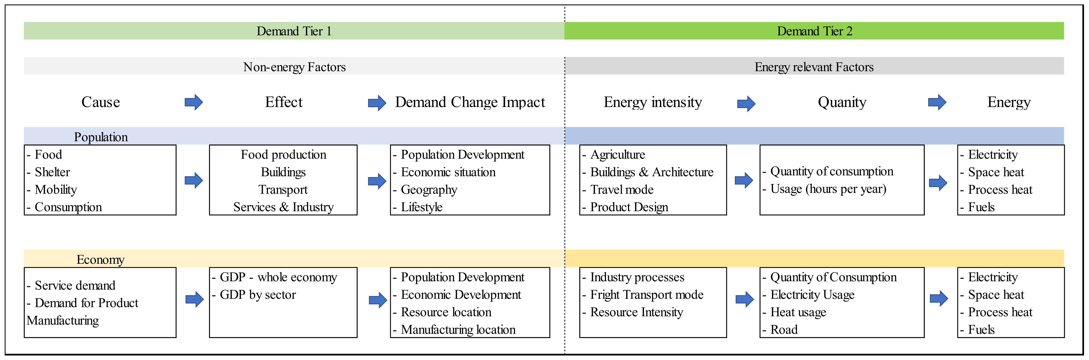
As in basic energy models, the main drivers of the energy demand are the development of the population and economic activity, measured in GDP. Figure 1 shows the basic methodology of the OECM demand module. The tier 1 inputs are population and GDP by region and sector. Whereas ‘population’ defines the number of individual energy services, which determines the energy required per capita, the economic activity (in GDP) defines the number of services and/or products manufactured and sold. The tier 1 demand parameters are determined by the effect that a specific service requires. For population, the demand parameters are defined by the need for food, shelter (buildings), and mobility and, depending on the economic situation and/or lifestyle of the population, the demand for goods and services.

Figure 1. Tier 1 and tier 2 input parameters for the assessment of energy demand.

Economic activity (measured in GDP) is a secondary input, and is directly and indirectly dependent upon the size of the population. However, a large population does not automatically lead to high economic activity. Both population and projected GDP are inputs from external sources, such as the United Nations or the World Bank. The tier 1 input parameters themselves are strictly non-technical. For instance, the need to produce food can be satisfied without electricity or (fossil) fuels, food production is a service that can be provided with a human workforce

The tier 2 demand parameters are energy-relevant factors, and describe technical applications, their energy intensities, and the extent to which the application is used. For example, if passenger road transport is required, the technical application ‘light duty vehicle (LDV)’ is chosen to satisfy the demand.

In this example, the energy intensity for an LDV with an internal combustion engine (ICE) is, for example, 1.5 MJ/km. The use of the application (=vehicle) is 15,000 km per year, which defines the demand (1.5 MJ/km × 15,000 km/yr = 22,500 MJ/yr). The application, in this example, an LDV with ICE, can be replaced with another technology, such as an electric vehicle with a reduced energy intensity of 0.5 MJ/km. The transport energy demand decreases, while the transport service (15,000 km) remains stable. In a second step, the actual transport service can be reduced or increased, or shifted to another transport mode (such as light rail) by the modeler.

This very basic and simple principle is used for every application in each of the main sectors: residential + buildings, industry, and transport. Those sectors are broken down into multiple sub-sectors, such as aviation, navigation, rail, and road for transport, and further into applications, such as vehicle types. The modular programming allows the addition of as many subsectors and applications as required.

3.5.2. Structure of the Demand Module

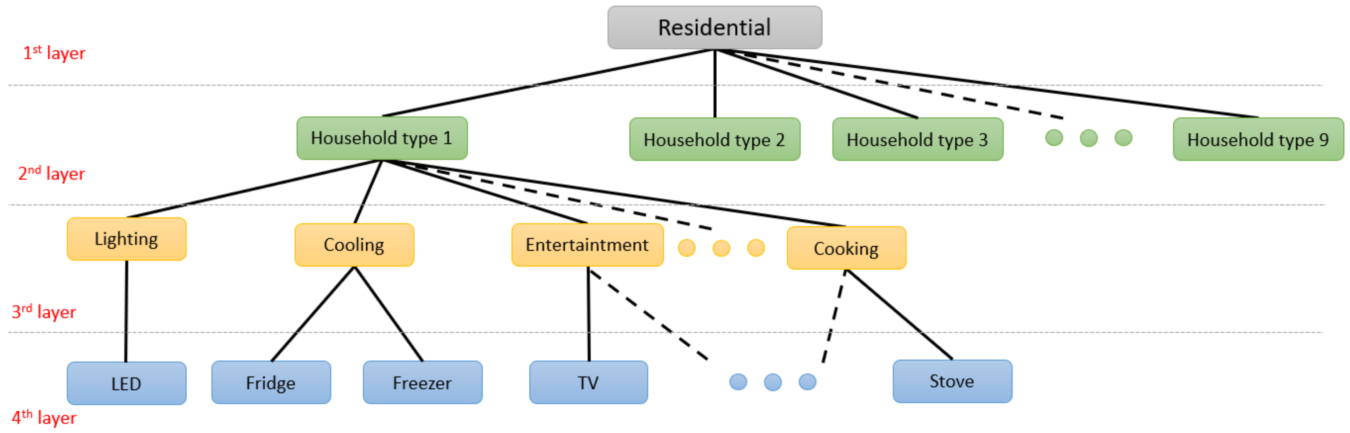
Each of the three sectors, residential & buildings (R), industry (I) and transport (T), has standardized sub-structures and applications. The residential sector R (first layer) has a list of household types (second layer) and each household type has a standard set of services (third layer), such as ‘lighting’, ‘cooling’ or ‘entertainment’. Finally, the applications for each of the services are defined (fourth layer), such as refrigerator or freezer for ‘cooling’. The energy intensity of each application can be altered by the modeler to reflect the status quo in a certain region and/or to reflect improvements in energy efficiency. An illustrative example of the residential sector layers is shown in Figure 2.

Figure 2. Residential sector sub-structures.

Figure 3 shows an example of the model structure of the industry sector. In the second layer, there are different industries—the OECM uses the GICS classification system for industry sub-sectors. The quantity of energy for each of the sub-sectors is driven by either GDP or the projected quantity of a product, such as the tons of steel produced per year. The market shares of specific manufacturing processes are defined and each process has a specific energy intensity for electricity, (process) heat, and/or fuels.

Figure 3. Calculation of Industry energy demand.

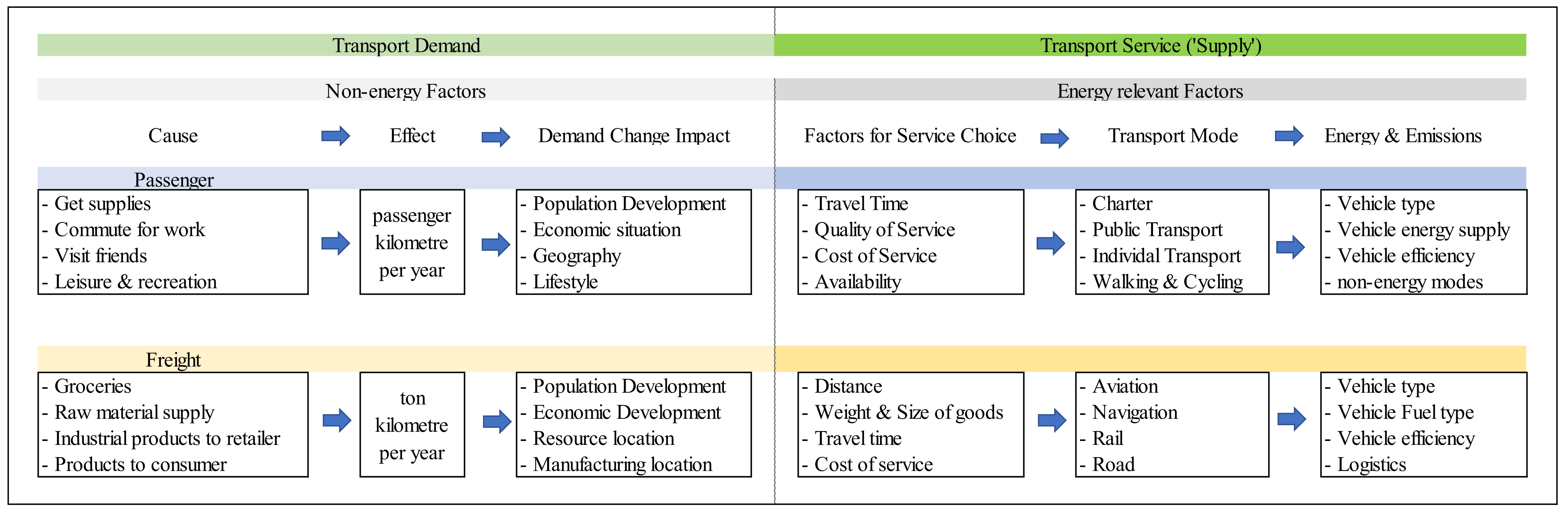
Figure 4 shows the structure for the transport sector. Again, the demand is driven by ‘non-energy’ factors, such as passenger-kilometers and freight-kilometers, and energy-related factors, such as the transport mode and the energy intensity for the different vehicle options.

Figure 4. Calculation of Transport energy demand.

3.6. Supply Module

After the demand has been calculated, the supply of electricity, heat, and fuels is calculated. The supply does not differentiate between different demand sectors. Therefore, the electricity demand for all sectors—residential, industry, and transport—is summed and is supplied as a whole. Consequently, no specific electric generation mix for the transport sector, for example, is considered.

The supply module consists of three main elements: supply technologies, storage technologies, and the infrastructure for the power supply (capacities of power lines). For the generation of electricity and heat, the program considers all the technologies of the energy market, from both renewable and non-renewable sources. In addition to the generation of pure electricity and heat, the entire range of combined heat and power systems is covered.

Storage technologies include batteries and the use of hydrogen from electrolyzers. The calculation of heat storage is possible, but has not yet been used in the OECM scenarios.

A dispatch strategy is defined for electricity and heat generation that reflects the market and policy factors. Whether electricity from photovoltaics (PV) and onshore and offshore wind turbines have priority dispatch, ahead of fossil fuel power plants and how storage systems are used, can be determined. Each technology has a specific conversion efficiency.

Heat generation technologies are also defined by the temperature levels they can provide. For example, residential solar collectors can only supply low-temperature heat and will therefore not be considered for high-temperature process heat.

The regional energy demand—as defined in the previous section—can be met by neighboring regions, with importation or, in the case of oversupply, exportation to them. The extent to which electricity can be imported or exported from one region to another is defined by the capacity of regional interconnections, which represent the currently available power line capacities. When variable renewable power generation must be curtailed because the capacity of the power line is restricted, MATLAB documents the quantity, in terms of both capacity (MW) and duration (hours per year). If the curtailment exceeds a certain fixed proportion of the annual usage hours, the additional power line capacity required is increased and documented by the program.

3.6.1. Dispatch Module

The methodology of the dispatch module of the MATLAB-based One Earth Climate Model is based on the previous version of the model [7]. The key inputs are related to the supply technologies, storage types, the dispatch strategy, and the interconnections among regions for possible power exchange (Table 6). Different supply technologies can be selected, each with its technical characteristics, including its efficiency, available installed capacity, fuel type, and regional meteorological data (solar radiation or wind speed) (Table 7). Meteorological data define the capacity factors of solar and wind energy generators as their levels of availability at a 1 h resolution for an entire year.

Table 6. Example of generation and storage technologies.

Generation			Storage
Power Plants	Combined Heat and Power Plants	Heating Plants	Electrical	Thermal	Hydrogen
Hard coal	Hard coal	Coal	Lithium battery	Water tank	Tank
Lignite	Lignite	Lignite	Pumped hydro	Molten salt
Gas	Gas	Gas
Oil	Oil	Oil
Diesel	Biomass	Biomass
Biomass	Geothermal	Solar collectors
Hydro	Hydrogen	Geothermal
Wind		Hydrogen
PV
Solar
Geothermal
Solar thermal
Ocean energy
Hydrogen

Table 7. Input parameters for the dispatch model.

Input Parameter
LCluster	Load cluster	[MW]
LInterconnection	Maximum power-line capacity (import/export)	[MW]
LInitial		[MW]
CapVar.RE	Installed capacity of Variable Renewables	[MW]
MeteoNorm	Meteorological data for solar and wind	[MW/MWINST]
LPost_Var.RE	Load after Variable Renewable supply	[MW]
CapStorage	Storage capacity	[MW]
CapFactMax_Storage	Maximum capacity factor for storage technologies	[h/yr]
LPost_Storage	Load after Storage supply	[MW]
CapDispatch	Capacity of Dispatch Power Plants	[MW]
CapFactMax_Dispatch	Maximum capacity factor for Dispatch Power Plants	[h/yr]
LPost_Dispatch	Load after Dispatch Power Plant supply	[MW]
CapInterconnection	Interconnection capacity	[MW]

Table 8, Table 9, Table 10 and Table 11 provide an overview of the possible supply technologies and examples of different dispatch scenarios. The left column shows the available technology options and the right column provides an example of the priority order chosen by the user of OECM 2.0.

Table 8. Output parameters for the dispatch model.

Output Parameter
LInitial	Initial load (cluster)	[MW]
LPost_Var.RE	Load after Variable Renewable supply	[MW]
SEXECC_VAR.RE	Access supply Renewables	[MW]
LPost_Storage	Load after Storage supply	[MW]
SStorage	Storage Requirement/Curtailment	[MW]
CapFactActual_Storage	Utilization factor for storage	[h/yr]
LPost_Dispatch	Load after Dispatch Power Plant supply	[MW]
SDispatch	Dispatch requirement	[MW]
CapFactActual_Dispatch	Utilization factor for Dispatch Power Plants	[h/yr]
LPost_Interconnection	Load after Interconnection supply	[MW]
SInterconnection	Interconnection requirement	[MW]
CapFactActual_Interconnection:	Utilization factor for Interconnection	[h/yr]

Table 9. Technology groups for dispatch order selection.

Technology Options	Input
List of technology options in OECM 2.0	Examples of the priority order chosen by user of OECM 2.0
1. Variable Renewables	Variable Renewables
2. Storage	Dispatch Generation
3. Dispatch Generation	Storage
4. Interconnector	Interconnector

Table 10. Technology options—variable renewable energy.

Variable Renewable Power Technology Options	Input: Assumed Order of Generation Priority
List of Technology Options in OECM 2.0	Examples of the Priority Order Chosen by User of OECM 2.0
1. Photovoltaic—roof top	Photovoltaic—utility scale (2)
2. Photovoltaic—utility scale	Photovoltaic—roof top (1)
3. Wind—onshore	Wind—offshore (4)
4. Wind—offshore	Wind—onshore (3)
5. CSP (dispatchable)	CSP (5)

Table 11. Technology options—dispatch generation.

Dispatch Generation Technology Options	Input: Assumed Order of Generation Priority
List of technology options in OECM 2.0	Examples of the priority order chosen by user of OECM 2.0
1. Bioenergy	Hydropower (3)
2. Geothermal	Bioenergy (1)
3. Hydropower	CoGen Bio energy (7)
4. Ocean	Geothermal (2)
5. Oil	CoGen Geothermal (8)
6. Gas	Ocean (4)
7. CoGen Bio energy	Gas (6)
8. CoGen Geothermal	CoGen Gas (9)
9. CoGen Gas	Coal (11)
10. CoGen Coal	CoGen Coal (10)
11. Coal	Brown Coal (12)
12. Brown coal	Nuclear (13)
13. Nuclear	Oil (5)

The supply technologies can be either dispatchable (e.g., gas power plants) or non-dispatchable (e.g., solar PV without storage). The model allows the order in which the supply technologies and storage functions are used to supply the demand. Storage and interconnections cannot be selected as the first elements of supply (Table 8).

Concentrated Solar Power (CSP) plants can be operated with on-site storage technologies and are therefore dispatchable. However, those storage capacities are limited, therefore the MATLAB model classifies CSP plants as Variable Renewable Power Plants. The dispatch order of all power plant technologies is interchangeable. In case solar and wind power plants exceed demand, or other power plants have priority dispatch, the amount of curtailed electricity is documented in MATLAP. Alternatively, surplus production can either be distributed to other regions (=cluster) or assigned to various storage technologies. Different storage technologies are defined by efficiencies, maximum charging and discharging capacities as well as the storage volume in MWh (Table 12).

Table 12. Technology options—storage technologies.

Storage Technology Option	Input: Assumed Priority Order Storage Technologies
List of technology options in OECM 2.0	Example for the priority order chosen by user of OECM 2.0
1. Battery	Hydro Pump (2)
2. Hydro Pump	Battery (1)
3. H2	H2 (3)

Limitations: The OECM 2.0 can calculate required power grid transport capacities between individual regions (clusters). However, network services such as inductive power supply and frequency control must be calculated in a dedicated models as the OECM is not designed for this.

3.6.2. Regional Interconnections

The available electricity transport capacities between two geographically connected regions are determined in relation to the generation capacity installed in the region. The required electricity transport capacities within a region cannot be taken into account. Therefore, a region itself is considered a ‘copper plate’; a transmission system where electricity can flow unconstrained from any generation site to any demand site is found in most energy modeling tools [27]. This simplification is required to achieve a short calculation time, while maintaining a high technical and time resolution. The algorithm devised for the function of the interconnectors is based on the following information for each region:

-

Unmet load in the region;

-

Excess generation from other regions;

-

Interconnection capacity between the undersupplied region and each of the other regions;

-

Priority of the closest region(s) in exporting power to the undersupplied region.

Electricity demand and supply for each hour of the year are calculated for all regions. In case of a regional undersupply (=unmet load), regions with excess generation are identified. The nearest region with the highest surplus is chosen as the priority electricity supplier. If the electricity supply is still not sufficient, another region with the second highest surplus is chosen. In general, the local electricity supply has priority over electricity export. Only regions that are geographically connected can exchange electricity.

The amount of electricity transported between regions is calculated in megawatts for each hour of the year. The maximum capacity required for the import or export of electricity defines the required transmission capacity. The interconnected capacity can be defined as an input. If the required interconnection capacity exceeds the determined transmission capacity, electricity transfer will be curtailed. This curtailment is recorded and defines transmission capacity increases.

Similar to the supply technologies, different storage technologies (electrical, thermal, or hydrogen) can be defined and selected together with their technical characteristics, such as round-trip efficiency, new or installed capacities in each year of the modelled period, lifetime, maximum depth of discharge, maximum energy out in a time step, and costs. When the total energy delivered by the supply technologies in a region does not meet the demand, energy is discharged from storage (if the storage technology has energy available), following the constraints of the storage operation (maximum energy out per time step, maximum depth of discharge, maximum depth of charge, state of charge) and the order of operation for the defined storage technologies. In the case of a demand deficit after storage, electricity from other regions will be imported. When there is surplus energy generation, the surplus will charge any storage appliances (if available), according to the same constraints of energy storage operation and sequential order.

4. Model Architecture

In this section, we describe how the elements mentioned above in Section 3 can be incorporated in MATLAB. The MATLAB model has an object-oriented structure and two modules, to calculate demand and supply, which can be operated independently of each other. Thus, an energy demand analysis independent of specific supply options or the development of a supply concept based on demand from an external source is possible. Specifically, the architecture of the demand and supply modules developed are formally described below.

4.1. Demand Module Architecture in MATLAB

The demand module is implemented in MATLAB, a widely used programming language for mathematics and science computing. MATLAB allows the integration of a range of tools and databases, and has the flexibility to add and develop new functions. Specifically, the model has been developed using an object-oriented programming approach, allowing extensibility and modularity.

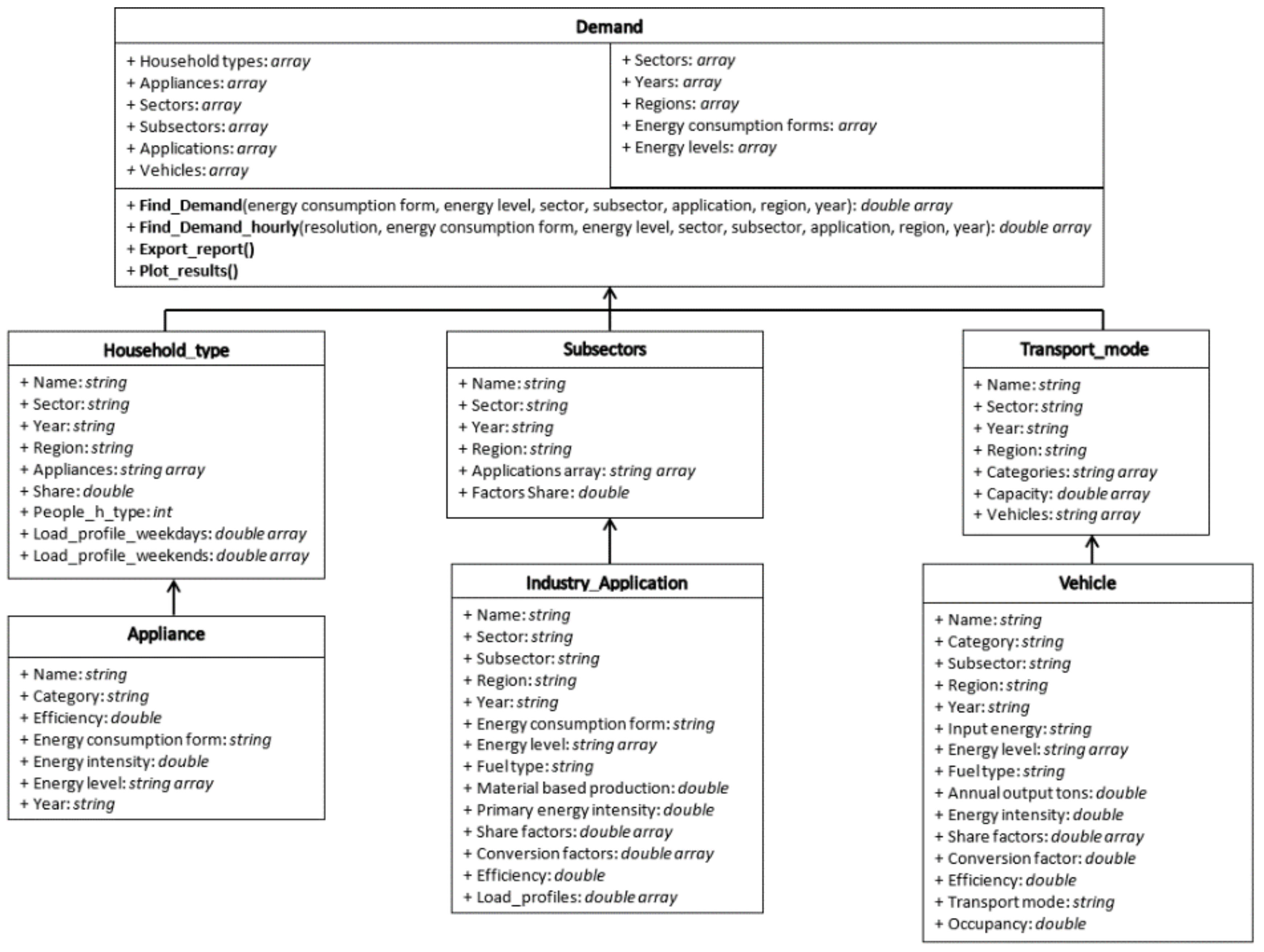
Figure 5 shows the developed demand module in MATLAB. In particular, the demand module encompasses seven classes:

Figure 5. A Unified Modelling Language (UML) diagram of the demand module in MATLAB, showing its classes, attributes, methods, and associations.

• Demand class: This is the main class, which describes the residential, industry, and transport sectors, objects that are defined by household type, sub-sector, and transport mode classes, respectively. The attributes that define this class include a range of years, energy consumption forms, energy levels, list of sectors, household types, sub-sectors, applications, appliances, and vehicles. The demand class also has two main types of methods: (i) calculation demand methods, and (ii) printing results methods. The calculation methods use equations and algorithms to calculate and find the demand. For example, the ‘Find Demand’ method can be used to find a wide range of calculations and outputs, e.g., the electricity demand of a group of households for a specified year. The calculation method can calculate the demand for single or aggregated sectors, sub-sectors, or applications, for a single year or a range of years, unique or multiple forms of energy consumption, and single or various types of vehicle categories. The printing results methods can be used to export the results into an Excel spreadsheet or to plot the results using the MATLAB interface. Thus, the outputs of the demand module can be either pre-defined graphs, tables, or data for a standardized report. See Table 13 for a brief description of each method in this class.
  Table 13. Dispatch module–inputs, intermediate outputs and outputs.

  Inputs, Intermediate Outputs, Outputs
  Inputs	Maximum capacity for interconnections among regions	[MW]
  Inputs	Initial load (cluster or region)	[MW]
  Inputs	Technical specifications of supply technologies and storage strategies
  Inputs	Meteorological data
  Intermediate output	Dispatch order of technologies
  Intermediate output	Load after Variable Renewable supply	[MW]
  Intermediate output	Load after Storage supply	[MW]
  Intermediate output	Load after Dispatch Power Plant supply	[MW]
  Intermediate output	Load after Interconnection supply	[MW]
  Output	Deficit and curtailment	[MWh]
  Output	Renewable penetration	[MWh]

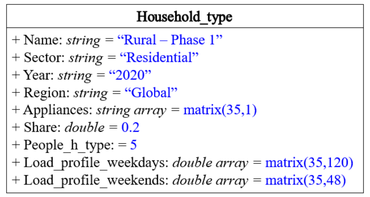
• Household and appliance classes: These classes are used to define the residential sector. The appliance objects are embedded within the household-type objects (Figure 6). Attributes include names, sectors, and regions, which are defined as string inputs (i.e., text or character inputs), or numerical inputs, which are defined as int (i.e., integers) or double (i.e., numeric variables holding numbers with decimal points). Attributes can also include arrays of strings or double values. Array variables are helpful in input time–series data, such as load profiles. Because households and appliances have their own classes, this architecture is flexible and allows the addition of households with different attributes and different types of appliances.
  

  Figure 6. An example of a Household type object, showing the assigned attributes.
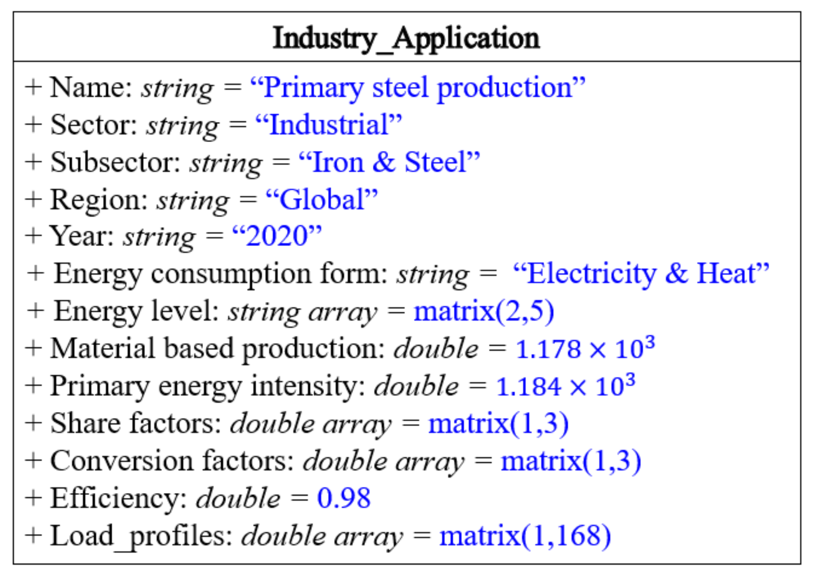
• Sub-sector and industry application classes: These classes are used to define the industry sector. The industry application objects are embedded within the sub-sector objects. As shown in Figure 7, these classes have their own lists of attributes. Therefore, the module developed can accommodate different types of sub-sectors (e.g., steel, cement, etc.,) and incorporate various types of applications under each sub-sector.
  

  Figure 7. An example of an Industry application object, showing the assigned attributes.
• Transport modes and vehicle classes: These classes are used to define the transport sector. The vehicle objects are embedded within the transport mode objects. Therefore, multiple types of transport modes can be defined, such as aviation and navigation, as well as various types of vehicles, such as planes and cruise ships.

Figure 6 and Figure 7 show the high-level class definitions for residential and industry sub-sector objects, respectively. The blue-marked text indicates the defined value for each attribute. For example, one household object with five residents is defined by the name “Rural–Phase 1”, and it has a list of 35 appliance objects, defined with a string array. It is assigned a share factor for 2020 of 0.2, which means that 20% of the households in that specific region and year are defined by this type of household and its attributes. Furthermore, 24 h load profiles are defined for each application for every day, with numerical arrays. For example, weekend load profiles have a size of 35 rows and 48 columns, representing 35 applications and 24 time slots for each weekend day.

The object-oriented architecture allows all these input attributes to be updated or modified easily. These attributes can also be read from a pre-defined Excel spreadsheet. This would facilitate a data input process that follows the array structure, such as the load profile.

Figure 7 shows an example of an industrial application object, which belongs to the sub-sector iron & steel. In this case, the energy consumption form is defined as electricity and heat, which means that it considers the electrical and heat demand. The ‘share factors’ represent the portion of the demand assigned to electricity and heat. The energy level array also allows the pre-defined network to which the application is connected to be defined, as well as the temperature levels. In this particular case, the demand is defined based on the total annual primary energy intensity and the material-based production, which are 1184 GJ/tons and 1178 Mt, respectively, for the specified region and year. The input and output units must be pre-defined when the MATLAB modules are initialized. Other attributes that can be assigned are conversion factors, such as from the primary energy to final energy via an efficiency factor.

Additional attributes and methods can be defined for each class if required and the data are available. Therefore, the demand module class can be extended by defining new classes, attributes and methods.

4.2. Supply Module Architecture in MATLAB

Analogous to the demand module, inputs can be made directly into the supply module via MATLAB or a standardized Excel sheet. The supply module in MATLAB is also based on an object-oriented structure, in which classes and the objects belonging to those classes are built based on attributes and methods.

Figure 8 shows the UML class diagram for the supply module developed in MATLAB. Specifically, the supply module has three main classes:

Figure 8. A UML diagram of the supply module in MATLAB, showing its classes, attributes, methods, and associations.

• Supply class: This is the main class and it is built on the supply and storage technology objects. Attributes that describe the supply class include years, regions, energy supply forms, fuels, and generation and storage technologies. The supply class has two main types of methods: (i) calculation supply methods; and (ii) printing results methods. The calculation methods implement equations and algorithms to calculate the dispatch and fuel consumption. Table 14 presents a brief description of each method.
  Table 14. Methods within the demand class.

  Type of Method	Method	Description
  Calculation	Find Demand() and Find_Demand_hourly()	These methods calculate the annual or hourly aggregated energy demand for the specified region and energy form (i.e., power, heat, or hydrogen). The calculations can be aggregated by sector, sub-sector, transport mode, or any other object class.
  Printing results	Export_report()	This method exports the specified results to external Excel spreadsheets and can be used to print results on pre-defined report tables.
  Printing results	Plot_results()	This method can be used to plot results using the MATLAB interface.

• Supply technology class: This class is used to define supply technologies. Attributes include name, type, efficiency, year, region and energy supply form and are defined as text inputs. Additional attributes are defined as numerical inputs, such as lifetime, cost and capacity factors. The structure adopted allows the addition of new attributes if required. This class has methods that are used by the main supply class to calculate the primary fuel, emissions, or installed capacity of a specific technology.
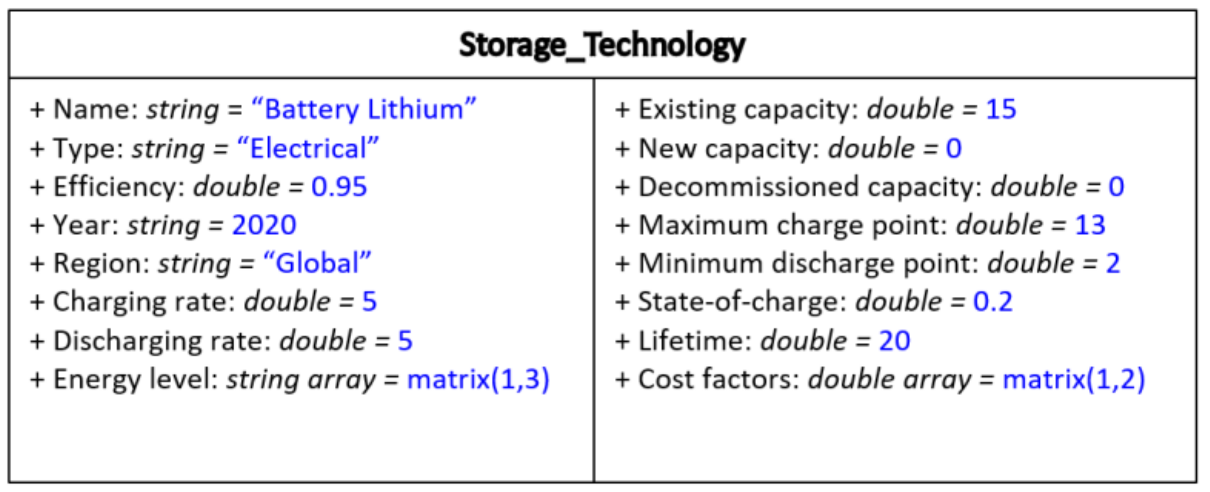
• Storage technology class: This class is used to defined storage technologies. The attributes include name, type, efficiency, year, region and energy storage form and are defined as text inputs Other numerical attributes include charging and discharging rates, capacity, cost factors, and state of charge.

Figure 9 and Figure 10 show the high-level class definitions for supply technologies and storage objects, respectively. The text in blue indicates the defined value for each attribute. For example, the supply technology object in Figure 9 has the name “coal power plant”; its input energy is defined as hard coal, and the object is associated with the electricity energy form. The attributes in Figure 9 consider the year 2020 and a global scenario. For example, the existing capacity is defined as 989.5 GW and the decommissioned capacity is 23 GW. The lifetime of this object is 35 years.

Figure 9. An example of a supply technology object, showing the assigned attributes.

Figure 10. An example of a storage technology object, showing the assigned attributes.

An example of a storage object is shown in Figure 10. The attributes of this object include text inputs, such as its name “battery lithium” and its type “electrical”. This object has numerical attributes such as the efficiency (equal to 0.95 for this object), and the charging and discharging rates (fixed at 5 kW). Note that the units for each attribute are defined when the module is initialized in MATLAB.

The supply module architecture developed is flexible to accommodate different types of supply and storage technologies. Additional attributes or methods can be added easily to the model.

5. OECM 1.5 °C Transport Trajectory

This section provides the calculated results for the OECM 1.5 °C transport pathway, calculated with the described methodology.

5.1. OECM 1.5 °C Transport Demand Calculation

The global transport energy demand was calculated with the economic and technical parameters shown in Table 3. Transport mode shifts for passenger and freight transport are assumed. These assumptions are manual inputs in MATLAB. Table 15 and Table 16 show the assumed changes in the transport modes relative to 2019, for passenger and freight transport. The main driver of the transport mode shifts is energy efficiency, towards lower energy intensities per kilometer.

Table 15. Methods within the supply class.

Type of Method	Method	Description
Calculation	Find_Supply() and Find_Supply_hourly()	These methods calculate the annual or hourly aggregated energy supply for the specified region and the energy form (i.e., power, heat, or hydrogen). The calculations can be made by individual or group supply technology type or storage type. These methods can also be used to calculate the emissions and primary fuel associated with each supply technology.
Calculation	Find_Share()	This method calculates the share factor results for pre-defined supply scenarios; for example, the share factors of power generated from renewable energy sources and non-renewable sources. Another example is the portion of the transport sector that requires electricity or hydrogen.
Calculation	Find_Economy()	This method calculates the costs associated with supply technologies.
Calculation	Get_fuel_total()	This method calculates the total fuel or total primary fuel required for demand and supply.
Calculation	Get_emission_total()	This method calculates the total emissions, considering all the demand sectors and supply technologies.
Calculation	Find_losses()	This method calculates the losses for a specified energy form. For example, it can be used to calculate the electricity losses or heat losses arising from transport and distribution.
Calculation	Find_capacities()	This method calculates the installed capacity for a specified technology when decommission or new capacity parameters have been defined.
Calculation	Reliability()	This method calculates the total energy deficit and curtailment based on the total demand and generation, for the specified energy form.
Printing results	Export_report()	This method exports the specified results to external Excel spreadsheets and can be used to print results on pre-defined report tables.
Printing results	Plot_results()	This method can be used to plot results using the MATLAB interface.

Table 16. Global: Development of behavioral changes in passenger travel (based on pkm) by transport mode.

Change in % of 2020 Demand	2019	2025	2030	2040	2050
Rail	100%	117%	136%	221%	360%
Road	100%	112%	109%	105%	94%
Domestic Aviation	100%	101%	96%	71%	47%
Domestic Navigation	100%	101%	94%	81%	69%
Total	100%	111%	109%	108%	101%

The energy demands for aviation, navigation and road transport are calculated with the documented input parameters and the methodology shown in Figure 4. Table 17 shows the results broken down into three transport modes and separated into passenger and freight transport. The energy demands for the manufacture of airplanes, ships and road vehicles are provided. The energy demand for the actual transport services is calculated on the basis of the transport kilometers required, the vehicles chosen for each transport mode and the assumed improvements in energy efficiency for the transport technologies.

Table 17. Global: Development of changes in freight logistics (based on tkm) by transport mode.

Change in % of 2020 Demand	2019	2025	2030	2040	2050
Rail	100%	133%	186%	238%	305%
Road	100%	110%	107%	103%	92%
Domestic Aviation	100%	102%	98%	76%	51%
Domestic Navigation	100%	103%	97%	85%	75%
Total	100%	106%	103%	96%	89%

In contrast, the energy demand for the manufacture of transport equipment, (e.g., car manufacture) is calculated from the assumed development of GDP and the standard energy efficiencies, in MJ per $GDP.

The technical resolution of standard energy assessment tools, such as REMIND [18] see Section 2.1), cannot differentiate the energy demand for specific manufacturing processes (such as car manufacture), and the energy demand would be part of the industry sector. Financial institutions and institutional investors that have agreed to net-zero targets require sector-specific benchmarks for clearly defined investment sectors to set their targets. However, those investment sectors are not consistent with the breakdown of the demand sectors used in standard energy statistics. Therefore, the OECM methodology presented here closes the knowledge gap and provides a flexible tool with which to calculate benchmarks for various combinations of sub-sectors on the basis of standard energy statistical databases, such as the IEA World Energy Balances [28].

5.2. OECM 1.5 °C Transport Energy Supply Calculation

After the energy requirements of the different sectors are calculated, we turn to the supply of energy. Table 18 shows the energy supply requirements for the transport modes analyzed and the manufacture of transport equipment. The chosen application, which is in the context of transport the various vehicle technologies, determines the change in the energy sources required, e.g., from petrol or diesel to bio-diesel, hydrogen, or electricity.

Table 18. Transport energy demand by transport mode under the OECM 1.5 °C pathway.

Parameter	Units	2019	2025	2030	2040	2050
Aviation
Air Freight: Energy Demand	[PJ/yr]	1445	911	809	595	430
Air Passenger: Energy Demand	[PJ/yr]	13,004	8195	7279	5359	3866
Energy Demand—Airplane Manufacture	[PJ/yr]	165	171	201	270	336
Navigation
Shipping Freight: Energy Demand	[PJ/yr]	11,067	10,659	11,023	11,233	11,554
Shipping Passenger: Energy Demand	[PJ/yr]	833	802	830	846	870
Energy Demand—Ship & Yacht Manufacture	[PJ/yr]	235	244	287	385	480
Road
Road Freight: Energy Demand	[PJ/yr]	38,598	28,937	26,027	16,736	11,058
Road Passenger: Energy Demand	[PJ/yr]	53,302	50,113	39,315	19,000	13,787
Energy Demand—Road Vehicle Manufacture	[PJ/yr]	1834	1905	2238	3004	3745
Total Energy Demand Transport	[PJ/yr]	120,482	101,937	88,008	57,428	46,125

The demand for fuels and fuel types is directly related to the vehicle technology selected, and is therefore not technology neutral for the supply side. However, a shift towards synthetic fuels and/or electricity will increase the electricity demand, but will not influence the electricity generation technology, as such. The development of the electricity generation technology mix is determined by the carbon intensity of the generation technology, the locally available renewable energy resources, and the available infrastructure.

Increased electrification significantly reduces the final energy demand of the transport sector, whereas the actual transport service in terms of kilometers will remain stable for passenger transport (+1% between 2020 and 2050) and will increase for freight transport (+15% between 2020 and 2050).

The additional electricity demand of the transport sector is added to the overall power generation requirement and calculated with the OECM demand module described in Section 4.2. The global electricity supply shares, under the OECM 1.5 °C pathway, are shown in Table 19. The specific CO₂ emissions for electric vehicles, in CO₂ per kilometer, and for the production of hydrogen, are calculated with the average specific CO₂ emissions per kilowatt hour of generated electricity (carbon intensity of electricity). The same values for the electricity carbon intensity for each year are used for all sectors and industries analyzed, e.g., for transport, the steel industry, or residential electricity supply.

Table 19. Energy supply requirements for aviation, navigation, road transport and the manufacture of transport equipment.

Parameter	Units	2019	2025	2030	2040	2050
Aviation Supply
Air Freight Fuel: Fossil	[PJ/yr]	580	892	740	60	0
Air Freight Fuel: Renewable & Synthetic Fuels	[PJ/yr]	0	18	69	536	430
Air Freight Fuel: Renewables share	[%]	0%	2%	9%	90%	100%
Air Passenger Fuel: Fossil	[PJ/yr]	5224	8031	6660	536	0
Air Passenger Fuel: Renewable & Synthetic Fuels	[PJ/yr]	0	164	619	4823	3866
Air Passenger Fuel: Renewables share	[%]	0%	2%	9%	90%	100%
Navigation Supply
Shipping Freight Fuel: Fossil	[PJ/yr]	2270	10,425	7441	1460	0
Shipping Freight Fuel: Renewable & Synthetic Fuels	[PJ/yr]	11	235	3582	9773	11,554
Shipping Freight Fuel: Renewables share	[%]	0%	2%	33%	87%	100%
Shipping Passenger Fuel: Fossil	[PJ/yr]	171	785	560	110	0
Shipping Passenger Fuel: Renewable & Synthetic Fuels	[PJ/yr]	1	18	270	736	870
Shipping Passenger Fuel: Renewables share	[%]	0%	2%	33%	87%	100%
Road Transport Supply
Road Freight Fuel: Fossil	[PJ/yr]	36,898	26,621	23,513	3787	0
Road Freight Fuel: Renewable, Electric & Synthetic Fuels	[PJ/yr]	1700	2317	2514	12,949	11,058
Road Freight Fuel: Renewables share	[%]	4%	8%	10%	77%	100%
Road Freight Electricity: Fossil	[PJ/yr]	77	260	166	326	0
Road Freight Electricity: Renewables	[PJ/yr]	25	282	478	6081	5928
Road Freight Electricity share	[%]	0%	2%	2%	38%	54%
Road Passenger Fuel: Fossil	[PJ/yr]	50,954	46,485	34,491	4043	0
Road Passenger Fuel: Renewable, Electric, & Synthetic Fuels	[PJ/yr]	2348	3628	4825	14,957	13,787
Road Passenger Fuel: Renewables share	[%]	4%	7%	12%	79%	100%
Road Passenger Electricity: Fossil	[PJ/yr]	119	783	1154	8148	6783
Road Passenger Electricity: Renewables	[PJ/yr]	22	88	98	477	338
Road Passenger Electricity share	[%]	0%	2%	3%	45%	52%
Transport Equipment Manufacturing—Supply
Energy Demand—Transport Equipment	[PJ/yr]	2351	2442	2869	3852	4801
Electricity component	[PJ/yr]	1123	1038	1219	1637	2041
	[TWh/yr]	312	288	339	455	567
Transport Sector
Transport—Total Fuels	[PJ/yr]	101,386	101,021	86,932	55,984	44,325
Transport—Total Electricity	[PJ/yr]	1367	2451	3116	16,669	15,089
	[TWh/yr]	380	681	865	4630	4191

5.3. OECM 1.5 °C Transport Carbon Intensity Calculation

In the last step, the carbon intensity and the overall carbon emissions are calculated from the primary energy demand by fuel and sector, and from the emission factors for hard coal, brown coal (lignite), oil and gas shown in Table 20. The emission factor for fuels are stable across the entire time series, whereas the carbon intensity for electricity changes with the renewable electricity share (see data provided in Table 19, last row).

Table 20. Global electricity supply shares under the OECM 1.5 °C pathway.

		2019	2025	2030	2035	2040	2050
Coal	[%]	31%	17%	5%	1%	0%	0%
Lignite	[%]	7%	1%	1%	1%	0%	0%
Gas	[%]	24%	20%	15%	8%	4%	0%
Oil	[%]	3%	2%	1%	0%	0%	0%
Nuclear	[%]	10%	7%	4%	2%	0%	0%
Hydrogen (produced with renewable electricity)	[%]	0%	0%	0%	2%	2%	5%
Hydro power	[%]	16%	14%	13%	10%	9%	9%
Wind	[%]	5%	14%	22%	28%	32%	36%
Solar photovoltaic	[%]	2%	18%	30%	37%	36%	34%
Biomass	[%]	1%	3%	2%	2%	1%	1%
Geothermal	[%]	0%	1%	2%	2%	3%	3%
Solar thermal power plants	[%]	0%	1%	4%	8%	10%	10%
Ocean energy	[%]	0%	0%	0%	1%	1%	1%
Renewables share	[%]	25%	52%	74%	89%	95%	100%
Electricity Supply: Specific CO2 Emissions per kWh	[g CO2/kWh]	509	290	136	53	24	0

Table 21 shows the calculated carbon intensities and total carbon emissions by transport mode for the OECM 1.5 °C transport pathway. The total energy-related CO₂ emissions for, e.g., aviation per year, set the maximum annual CO₂ emission target, the cumulative emissions between 2020 and 2050, and the overall carbon budget under the 1.5 °C target (Table 22). The average specific CO₂ emissions per person kilometer and per ton-kilometer represent the technical benchmarks for aviation services.

Table 21. Emission factors used for the OECM 1.5 °C pathways.

	Units	Emission Factor
Lignite	[kt CO2/PJ]	111
Hard coal	[kt CO2/PJ]	93
Oil	[kt CO2/PJ]	75
Gas	[kt CO2/PJ]	56

Table 22. Transport: carbon intensity and total energy-related CO₂ emission by sector for the OECM 1.5 °C transport pathway.

		2019	2025	2030	2040	2050
Aviation
Air Freight: Emission Intensity	[g CO2/tkm]	2360	2092	1822	189	0
Air Freight: Total Emissions	[million t CO2/yr]	94	144	119	10	0
Air Passenger: Emission Intensity	[g CO2/pkm]	426	347	302	31	0
Air Passenger: Total Emissions (domestic)	[million t CO2/yr]	842	1295	1074	86	0
Aviation—Total	[million t CO2/yr]	0	18	69	536	430
Navigation
Shipping Freight: Emission Intensity	[g CO2/tkm]	15	15	10	2	0
Shipping Freight: Total Emissions	[million t CO2/yr]	738	3390	2420	475	0
Shipping Passenger: Emission Intensity	[g CO2/pkm]	5	4	3	1	0
Shipping Passenger: Total Emissions	[million t CO2/yr]	56	255	182	36	0
Shipping—Total	[million t CO2/yr]	2270	10,425	7441	1461	1
Road Transport
Road Freight: Emission Intensity	[g CO2/tkm]	105	90	80	14	0
Road Freight: Total Emissions	[million T CO2/yr]	3034	2189	1933	311	0
Road Passenger: Emission Intensity	[g CO2/pkm]	121	95	85	29	23
Road Passenger: Total Emissions	[million t CO2/yr]	4190	3822	2836	332	0
Road Transport—Total	[million t CO2/yr]	1778	2576	2680	13,275	11,058
Transport Equipment
CO2 Emissions—Road Vehicle Manufacture	[million t CO2/yr]	183	111	70	25	0
CO2 Emissions—Locomotive & Rail Vehicles Manufacture	[million t CO2/yr]	12	7	4	2	0
CO2 Emissions—Ships & Yachts Manufacture	[million t CO2/yr]	23	14	9	3	0
CO2 Emissions—Airplane Manufacturing	[million t CO2/yr]	16	10	6	2	0
Total CO2 Emissions	[million t CO2/yr]	234.2	142.8	89.3	32.0	0.0

6. Conclusions

To develop and calculate detailed energy scenarios for specific GICS-defined industry and service sectors requires energy models with a high technical resolution. There are currently no energy models on the market that calculate energy scenarios within the system boundaries defined according to the Global Industry Classification System (GICS). The OECM 2.0 closes this gap. The model architecture of the existing OECM 1.0 was modified to allow the integration of more technical parameters. The integration of new industrial areas required the calculation of energy consumption for sector-specific processes which led to a higher data volume. The OECM 2.0 uses MATLAB to process the data and to enable a flexible presentation of results.

In this paper, we documented the development and calculation of a 1.5 °C pathway for the GICS sector 2030 Transportation with the OECM 2.0 as a case study. The scenarios were further divided in 203010 Air Freight & Logistics, 20302010 Airlines (passenger transport), 203030 Marine transport and 203040 Road & Rail transport. The higher technical resolution of the OECM 2.0 allowed the development of an individual scenario for the different GICS sectors. However, the high technical resolution requires more detailed input parameters such as passenger-kilometers per year and the breakdown by vehicle type and transport mode. The required input data is not always available for all countries and/or industries. However, sufficient data is available to calculate the trajectories for aviation, shipping, road and rail transport on a global level.

6.1. OECM 2.0 Output and Area of Use

The additionality of OECM 2.0 provides a high resolution of the sector-specific parameters for both demand and supply, which are required as key performance indicators (KPIs) by the finance industry. Table 23 provides an overview of the main KPI parameters and the areas of their use, with a focus on the needs of institutional investors.

Table 23. Examples of energy-related key performance indicators (KPIs) for net-zero target setting, calculated with OECM 2.0 for four sectors.

Sector	Parameter	Units	Base Year 2019	Projection 2025, 2030, 2035, 2040, 2045, 2050
Commodities
Water Utilities	Water withdrawal	[billion m3/yr]	Input	Calculated projection with annual growth rates discussed with client
Chemical Industry	Economic development	[$GDP/yr]	Input
Steel industry	Product-based market projection	[tons steel/yr]	Input
Aviation	Passenger-kilometers	[million person km/yr]	Input
Energy Intensities
Water Utilities	Waste-water treatment	[kWh/m3]	Input	Technical target (KPI) Calculated with annual progress ratio based on technical assessment
Chemical Industry	Industry-specific energy intensity	[MJ/$GDP]	Input
Steel Industry	Energy intensity	[MJ/ton steel]	Input
Aviation	Energy intensity per transport service	[MJ/person km]	Input
Energy Demand
Water Utilities	Final energy demand	[PJ/yr]	Input	Output—industry-specific scenario(s)
Chemical Industry	Electricity demand	[TWh/yr]	Input
Steel Industry	Process heat demand by temperature level	[PJ/yr]	Input
Aviation	Final energy demand	[PJ/yr]	Input
	Total final energy demand	[PJ/yr]	Input
Energy Supply
Water Utilities	Electricity generation by technology	[TWh/yr]	Input	Output—based on developed scenario Supply for all (sub-)sectors.
Chemical Industry	(Process) heat by technology	[PJ/yr]	Input
Steel Industry	Fuel supply by fuel type	[PJ/yr]	Input
Aviation	Fuel supply by fuel type	[PJ/yr]
	Total final energy supply by fuel type	[PJ/yr]	Input
Energy-related Emissions
	Electricity—specific CO2 emissions	[gCO2/kWh]	Calculated	Output—KPI for utilities
	Electricity—total CO2 emissions	[t CO2/yr]	Calculated	Output—KPI for utilities
	(Process) heat—specific CO2 emissions	[gCO2/kWh]	Calculated	Output—KPI for industry
	Transport service energy	[g CO2/kilometer]	Calculated	Output—KPI for industry
	(Process) heat—total CO2 emissions	[t CO2/yr]	Calculated	Output—KPI for industry
Product specific Emission
Water Utilities	Emissions intensity	[kg CO2/m3]	Calculated	KPI—water utilities
	Total energy-related CO2 emissions	[t CO2]	Calculated	KPI—Water utilities
Chemical Industry	Emissions intensity	[kg CO2/$GDP]	Calculated	KPI—chemical industry
	Total energy-related CO2 emissions	[tCO2]	Calculated	KPI—chemical industry
Steel Industry	Emissions intensity	[kg CO2/t steel]	Calculated	KPI—steel industry
	Total energy-related CO2 emissions	[t CO2]	Calculated	KPI—steel industry
Aviation	Emission intensity	[kg CO2/passenger km]	Calculated	KPI—aviation industry
	Total energy-related CO2 emissions	[t CO2]	Calculated	KPI—aviation industry

Commodities and/or GDP are the main drivers of the energy demand for industries. The projection of, for example, the global steel demand in tons per year, over the next decades, are discussed with the industry and/or client. The OECM 2.0 can calculate either a single specific sector only or a whole set of sectors. In the case of global scenario development, various industry projections are combined to estimate both the total energy supply required and the potential energy-related emissions. Thus, a global carbon budget can be broken down into the carbon budgets of specific industries.

Energy intensities are both input data for the base year and a KPI for future projections. The effect of a targeted reduction in the energy intensity in a given year and the resulting energy demand and carbon emissions can be calculated, for example for the transport service industry.

All sector demands are supplied by the same energy supply structure in terms of electricity, process heat (for each temperature level) and total final energy. Finally, specific emissions, such as CO₂ per ton-kilometer, CO₂ per ton of steel or per cubic meter of waste water treatment, are calculated and can be used to set industry targets.

All input and output OECM data are available as MATLAB-based tables or graphs, or as standard Excel-based reports.

6.2. Model Dynamics

A detailed assessment of the energy demand based on industry products, such as the amount of steel or aluminum used and/or the economic projections (for example for sub-sectors of the chemical industry), combined with very high technical resolution, allows the development of the electricity and fuel demand to be comprehensively mapped with steadily increasing sector coupling. A high degree of electrification for heating and transport, to replace fuels, requires an energy scenario to be modelled that includes an electricity system analysis to assess the infrastructural changes required (i.e., the power grid). OECM 2.0 combines an integrated energy assessment tool with a system analysis module. Net-zero pledges for specific industries lead to more detailed energy scenarios for specific industry sectors. The steel industry, for example, favors hydrogen-based steel production, which will have a significant impact on the hydrogen demand and the electricity needed to produce it. OECM 2.0 takes this development into account and allows the modeler to change from a yearly to an hourly resolution when developing load curves for industries and/or the entire power system, when simulating an electricity supply with high shares of variable renewable power plants.

Another example in which a long-term scenario analysis must be combined with a system analysis occurs in the chemical industry. The switch to electrical process heat will not only significantly increase the power requirement, but also the power load. The decision to use electric or hydrogen-based process heat requires the analysis of the regional infrastructure to allow the development of a cost-effective solution.

The OECM 2.0 program is modular and currently includes 12 different industry sectors. Its expansion to more sectors and sub-sectors is possible without great effort, and thus increases the accuracy of the analysis of electricity and fuel requirements. This interaction between a technology change in one sector (e.g., to move to electric process heat) and the technical and cost implications for other sectors (e.g., power utilities and grid operators) is a central component of the model dynamics.

6.3. Limitations

Industry-specific energy intensities and energy demands are not available for a variety of industries. In particular, the energy intensities for sub-sectors of the chemical industry are either unavailable or confidential. A database of energy intensities is required to develop more detailed scenarios. Although energy intensities can be estimated based on the available data, the input parameters are usually derived from various sources, which may not follow the same methodology. Energy intensities based on GDP, for example, are calculated with either nominal GDP, real GDP, or purchasing power parity GDP. Furthermore, energy intensities can be provided as the final energy or primary energy. In some cases, this information is not available at all. A database of industry-specific energy demands and energy intensities, with a consistent methodology, is required to improve the accuracy of calculations in future research.