
Machine Learning for Prediction of Heat Pipe Effectiveness


 ,
,  ,
,  ,
,  ,
,  ,
,
Abstract
:1. Introduction
2. Materials and Methods
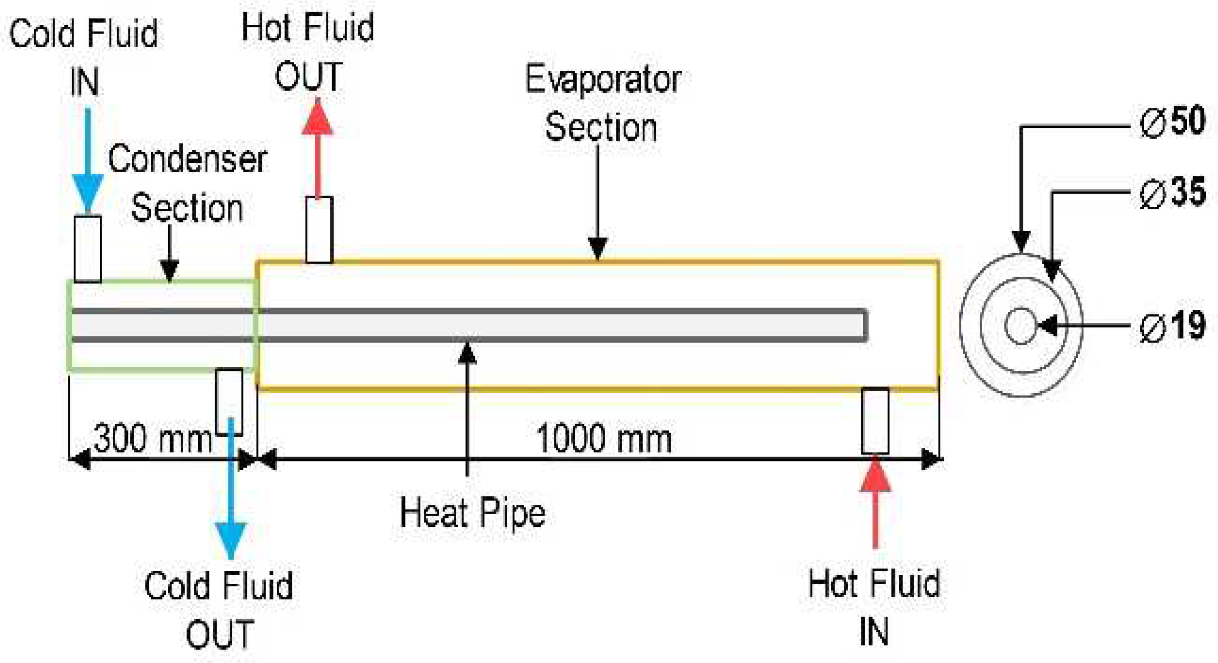
2.1. Fabrication
2.2. Experimental Procedure
2.3. Machine Learning Model
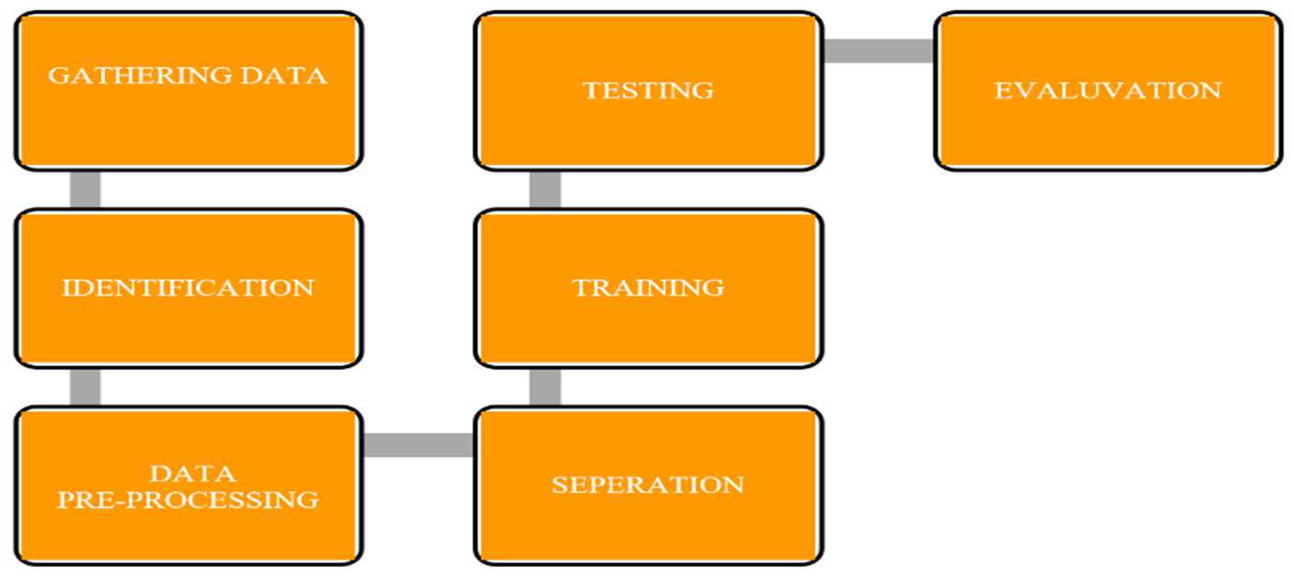
2.4. Identification and Pre-Processing of the Dataset
2.5. Separation, Training and Testing
2.6. Evaluation of Our Model
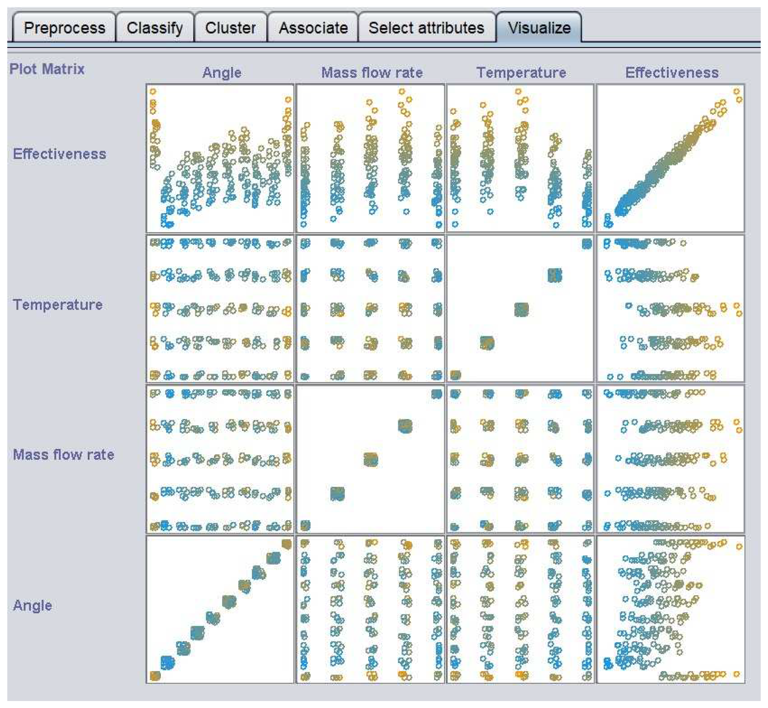
2.7. Dataset Description
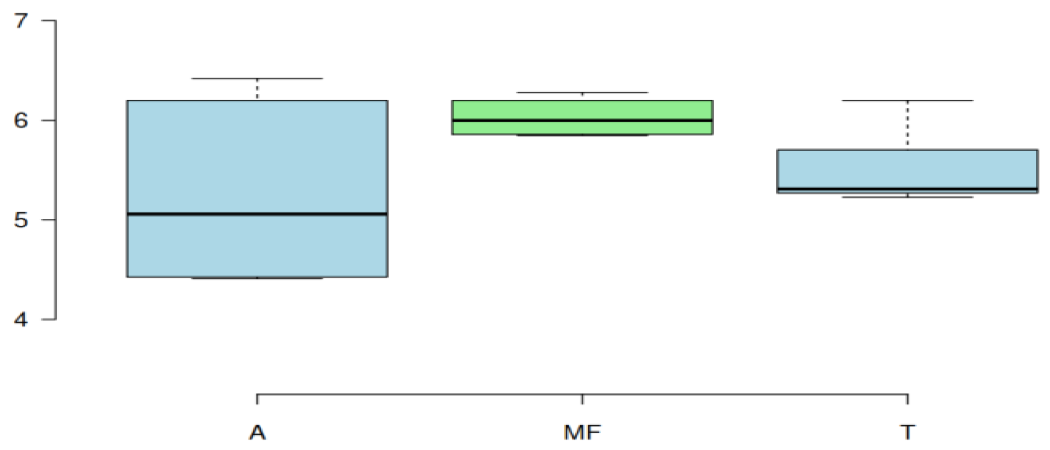
2.8. Dataset Separation
2.9. Precision of Prediction
3. Results and Discussion
4. Conclusions
Author Contributions
Funding
Institutional Review Board Statement
Informed Consent Statement
Data Availability Statement
Conflicts of Interest
References
- Noie-Baghban, S.H.; Majideian, G.R. Waste heat recovery using heat pipe heat exchanger (HPHE) for surgery rooms in hospitals. Appl. Therm. Eng. 2000, 20, 1271–1282. [Google Scholar] [CrossRef]
- Vasiliev, L.L. Heat pipes in modern heat exchangers. Appl. Therm. Eng. 2005, 25, 1–19. [Google Scholar] [CrossRef]
- Yang, F.; Yuan, X.; Lin, G. Waste heat recovery using heat pipe heat exchanger for heating automobile using exhaust gas. Appl. Therm. Eng. 2003, 23, 367–372. [Google Scholar] [CrossRef]
- Longo, G.A.; Righetti, G.; Zilio, C.; Bertolo, F. Experimental and theoretical analysis of a heat pipe heat exchanger operating with a low global warming potential refrigerant. Appl. Therm. Eng. 2014, 65, 361–368. [Google Scholar] [CrossRef]
- Wang, L.; Miao, J.; Gong, M.; Zhou, Q.; Liu, C.; Zhang, H.; Fan, H. Research on the Heat Transfer Characteristics of a Loop Heat Pipe Used as Mainline Heat Transfer Mode for Spacecraft. J. Therm. Sci. 2019, 28, 736–744. [Google Scholar] [CrossRef]
- Kempers, R.; Ewing, D.; Ching, C.Y. Effect of number of mesh layers and fluid loading on the performance of screen mesh wicked heat pipes. Appl. Therm. Eng. 2006, 26, 589–595. [Google Scholar] [CrossRef]
- Bastakoti, D.; Zhang, H.; Cai, W.; Li, F. An experimental investigation of thermal performance of pulsating heat pipe with alcohols and surfactant solutions. Int. J. Heat Mass Transf. 2018, 117, 1032–1040. [Google Scholar] [CrossRef]
- Patel, V.M.; Mehta, H.B. Experimental Investigations on the Effect of Influencing Parameters on Operating Regime of a Closed Loop Pulsating Heat Pipe. J. Enhanc. Heat Transf. 2019, 26, 333–344. [Google Scholar] [CrossRef]
- Jia, H.; Jia, L.; Tan, Z. An experimental investigation on heat transfer performance of nanofluid pulsating heat pipe. J. Therm. Sci. 2013, 22, 484–490. [Google Scholar] [CrossRef]
- Patel, V.K. An efficient optimization and comparative analysis of ammonia and methanol heat pipe for satellite application. Energy Convers. Manag. 2018, 165, 382–395. [Google Scholar] [CrossRef]
- Han, C.; Zou, L. Study on the heat transfer characteristics of a moderate-temperature heat pipe heat exchanger. Int. J. Heat Mass Transf. 2015, 91, 302–310. [Google Scholar] [CrossRef]
- Zhang, D.; Li, G.; Liu, Y.; Tian, X. Simulation and experimental studies of R134a flow condensation characteristics in a pump-assisted separate heat pipe. Int. J. Heat Mass Transf. 2018, 126, 1020–1030. [Google Scholar] [CrossRef]
- Lian, W.; Han, T. Flow and heat transfer in a rotating heat pipe with a conical condenser. Int. Commun. Heat Mass Transf. 2019, 101, 70–75. [Google Scholar] [CrossRef]
- Shabgard, H.; Bergman, T.L.; Sharifi, N.; Faghri, A. High temperature latent heat thermal energy storage using heat pipes. Int. J. Heat Mass Transf. 2010, 53, 2979–2988. [Google Scholar] [CrossRef]
- Savino, R.; Abe, Y.; Fortezza, R. Comparative study of heat pipes with different working fluids under normal gravity and microgravity conditions. Acta Astronaut. 2008, 63, 24–34. [Google Scholar] [CrossRef]
- Said, S.A.; Akash, B.A. Experimental performance of a heat pipe. Int. Commun. Heat Mass Transf. 1999, 26, 679–684. [Google Scholar] [CrossRef]
- Dixit, S. Study of factors affecting the performance of construction projects in AEC industry. Organization. Technol. Manag. Constr. 2020, 12, 2275–2282. [Google Scholar] [CrossRef]
- Dixit, S. Impact of management practices on construction productivity in Indian building construction projects: An empirical study. Organ. Technol. Manag. Constr. 2021, 13, 2383–2390. [Google Scholar] [CrossRef]
- Dixit, S. Analysing the Impact of Productivity in Indian Transport Infra Projects. IOP Conf. Ser. Mater. Sci. Eng. 2022, 1218, 12059. [Google Scholar] [CrossRef]
- Dixit, S.; Singh, P. Investigating the disposal of E-Waste as in architectural engineering and construction industry. Mater. Today Proc. 2022, 56, 1891–1895. [Google Scholar] [CrossRef]
- Dixit, S.; Stefańska, A. Digitisation of contemporary fabrication processes in the AEC sector. Mater. Today Proc. 2022, 56, 1882–1885. [Google Scholar] [CrossRef]
- Rahimi, M.; Asgary, K.; Jesri, S. Thermal characteristics of a resurfaced condenser and evaporator closed two-phase thermosyphon. Int. Commun. Heat Mass Transf. 2010, 37, 703–710. [Google Scholar] [CrossRef]
- Venkatachalapathy, S.; Kumaresan, G.; Suresh, S. Performance analysis of cylindrical heat pipe using nanofluids–An experimental study. Int. J. Multiph. Flow 2015, 72, 188–197. [Google Scholar] [CrossRef]
- Charoensawan, P.; Khandekar, S.; Groll, M.; Terdtoon, P. Closed loop pulsating heat pipes: Part A: Parametric experimental investigations. Appl. Therm. Eng. 2003, 23, 2009–2020. [Google Scholar] [CrossRef]
- Shang, F.; Fan, S.; Yang, Q.; Liu, J. An experimental investigation on heat transfer performance of pulsating heat pipe. J. Mech. Sci. Technol. 2020, 34, 425–433. [Google Scholar] [CrossRef]
- Wang, J.; Ma, Y.; Zhang, L.; Gao, R.X.; Wu, D. Deep learning for smart manufacturing: Methods and applications. J. Manuf. Syst. 2018, 48, 144–156. [Google Scholar] [CrossRef]
- Ademujimi, T.T.; Brundage, M.P.; Prabhu, V.V. A Review of Current Machine Learning Techniques Used in Manufacturing Diagnosis BT-Advances in Production Management Systems. In The Path to Intelligent, Collaborative and Sustainable Manufacturing; Lödding, H., Riedel, R., Thoben, K.-D., von Cieminski, G., Kiritsis, D., Eds.; Springer International Publishing: Cham, Switzerland, 2017; pp. 407–415. [Google Scholar]
- Zacarias, A.G.V.; Reimann, P.; Mitschang, B. A framework to guide the selection and configuration of machine-learning-based data analytics solutions in manufacturing. Procedia CIRP 2018, 72, 153–158. [Google Scholar] [CrossRef]
- Krishnayatra, G.; Tokas, S.; Kumar, R. Numerical heat transfer analysis & predicting thermal performance of fins for a novel heat exchanger using machine learning. Case Stud. Therm. Eng. 2020, 21, 100706. [Google Scholar]
- El-Said, E.M.S.; Elaziz, M.A.; Elsheikh, A.H. Machine learning algorithms for improving the prediction of air injection effect on the thermohydraulic performance of shell and tube heat exchanger. Appl. Therm. Eng. 2021, 185, 116471. [Google Scholar] [CrossRef]
- Wang, Z.; Zhao, X.; Han, Z.; Luo, L.; Xiang, J.; Zheng, S.; Liu, G.; Yu, M.; Cui, Y.; Shittu, S.; et al. Advanced big-data/machine-learning techniques for optimization and performance enhancement of the heat pipe technology—A review and prospective study. Appl. Energy 2021, 294, 116969. [Google Scholar] [CrossRef]
- Frank, E.; Hall, M.A.; Witten, I.H. The WEKA Workbench. Online Appendix for Data Mining: Practical Machine Learning Tools and Techniques, 4th ed.; Morgan Kaufmann: Burlington, VT, USA, 2016. [Google Scholar]
- Holman, J.P. Experimental Methods for Engineers, 8th ed.; McGraw-Hill’s: New York, NY, USA, 2012; p. 800. [Google Scholar]

| Properties | Methanol |
|---|---|
| Boiling point | 65 °C |
| Melting point | −97.9 °C |
| Latent heat of evaporation (λ) | 1055 kJ/kg |
| Density of liquid (ρl) | 792 kg/m3 |
| Density of vapour (ρv) | 1.47 kg/m3 |
| Thermal conductivity of liquid (kl) | 0.201 W/m °C |
| Vapor pressure (at 293 K) | 12.87 kPa |
| Viscosity of liquid (μl) | 0.314 × 10⁻³ Ns/m2 |
| Surface tension of liquid (σ) | 1.85 × 10⁻² N/m |
| Molecular weight (M) | 32 g/mol |
| Specific heat ratio (νv) | 1.33 |
| S. No | Factors | Minimum | Maximum | Mean | Std-Dev |
|---|---|---|---|---|---|
| 1 | Angle (A) | 0 | 90 | 45 | 28.78 |
| 2 | Mass flow rate (MF) | 40 | 120 | 80 | 28.341 |
| 3 | Temperature (T) | 50 | 70 | 60 | 7.085 |
| 4 | Effectiveness (Methanol) | 6.84 | 38.98 | 20.13 | 6.177 |
| S. No. | Subsets | A | MF | T |
|---|---|---|---|---|
| 1 | A | 1 | 0 | 0 |
| 2 | MF | 0 | 1 | 0 |
| 3 | T | 0 | 0 | 1 |
| 4 | A-MF | 1 | 1 | 0 |
| 5 | A-T | 1 | 0 | 1 |
| 6 | MF-T | 0 | 1 | 1 |
| 7 | A-MF-T | 1 | 1 | 1 |
| Categories | Algorithms | Full-Form |
|---|---|---|
| Functions | SLR | Simple Linear Regression |
| LMs | Least Median Square | |
| GP | Gaussian Processes | |
| MLP | Multilayer Perceptron | |
| RBFN | Radial basis Function Network | |
| RBFR | Radial basis Function Regressor | |
| SMOREG | Support vector machine Optimizer Regression | |
| Lazy | IBK | Instance Based Learner K |
| K star | K Star | |
| LWL | Locally Weighted Learning | |
| Meta | AR | Additive Regression |
| BREP | Bagging Reduced Error Pruning | |
| MS | Multi Scheme | |
| RC | Random Committee | |
| RFC | Random Filtered Classifier | |
| RSS | Random Subspace | |
| RBD | Random By Discretization | |
| STACKING | Stacking | |
| VOTE | Vote | |
| WIHW | Weighted Instances Handled Wrapper | |
| Rules | DT | Decision Table |
| M5R | M5R | |
| ZEROR | ZERO R | |
| Trees | DS | Decision Stump |
| M5P | M5P | |
| RF | Random Forest | |
| RT | Random Tree | |
| REP TREE | Reduced Error Pruning | |
| Misc. | IMC | Instance Mapped Classifier |
| SUBSETS | A | MF | T | ||||
|---|---|---|---|---|---|---|---|
| Categories | ALGORITHMS | MAE | RMSE | MAE | RMSE | MAE | RMSE |
| Functions | SLR | 4.972 | 6.139 | 5.075 | 6.212 | 4.456 | 5.660 |
| LR | 4.972 | 6.139 | 5.053 | 6.199 | 4.456 | 5.660 | |
| LMs | 4.974 | 6.421 | 5.080 | 6.229 | 4.432 | 5.686 | |
| MLP | 4.986 | 6.126 | 5.179 | 6.280 | 4.372 | 5.654 | |
| GP | 5.063 | 6.180 | 5.068 | 6.203 | 4.776 | 6.023 | |
| RBFN | 4.914 | 6.061 | 5.058 | 6.195 | 4.462 | 5.601 | |
| RBFR | 4.100 | 4.951 | 4.761 | 5.847 | 4.135 | 5.271 | |
| SMOREG | 4.983 | 6.248 | 5.093 | 6.263 | 4.405 | 5.704 | |
| IBK | 3.673 | 4.415 | 4.761 | 5.847 | 4.135 | 5.271 | |
| Kstar | 4.208 | 5.166 | 4.790 | 5.882 | 4.208 | 5.304 | |
| LWL | 3.900 | 4.691 | 4.815 | 5.903 | 4.136 | 5.274 | |
| Meta | AR | 3.728 | 4.475 | 4.764 | 5.851 | 4.131 | 5.268 |
| BREP | 3.701 | 4.458 | 4.793 | 5.878 | 4.125 | 5.284 | |
| MS | 5.053 | 6.199 | 5.053 | 6.199 | 5.053 | 6.199 | |
| RC | 3.673 | 4.415 | 4.761 | 5.847 | 4.135 | 5.271 | |
| RFC | 3.673 | 4.415 | 4.739 | 5.847 | 4.135 | 5.271 | |
| RSS | 3.707 | 4.446 | 4.783 | 5.871 | 4.131 | 5.274 | |
| RBD | 3.702 | 4.410 | 4.864 | 5.944 | 4.151 | 5.228 | |
| STACKING | 5.053 | 6.199 | 5.053 | 6.199 | 5.053 | 6.199 | |
| VOTE | 5.053 | 6.199 | 5.053 | 6.199 | 5.053 | 6.199 | |
| WIHW | 5.053 | 6.199 | 5.053 | 6.199 | 5.053 | 6.199 | |
| Rules | DT | 3.673 | 4.415 | 4.761 | 5.847 | 4.135 | 5.271 |
| M5R | 3.721 | 4.485 | 4.851 | 6.000 | 4.102 | 5.229 | |
| ZEROR | 5.053 | 6.199 | 5.053 | 6.199 | 5.053 | 6.199 | |
| Trees | DS | 4.567 | 5.613 | 4.979 | 6.065 | 4.152 | 5.317 |
| M5P | 3.843 | 4.632 | 4.873 | 5.997 | 4.115 | 5.229 | |
| RF | 3.671 | 4.417 | 4.770 | 5.859 | 4.136 | 5.271 | |
| RT | 3.673 | 4.415 | 4.761 | 5.847 | 4.135 | 5.271 | |
| REP TREE | 3.683 | 4.427 | 4.818 | 5.876 | 4.195 | 5.333 | |
| IMC | 5.053 | 6.199 | 5.053 | 6.199 | 5.053 | 6.199 | |
| SUBSETS | A-MF | A-T | MF-T | ||||
|---|---|---|---|---|---|---|---|
| Categories | ALGORITHMS | MAE | RMSE | MAE | RMSE | MAE | RMSE |
| Functions | SLR | 4.972 | 6.139 | 4.456 | 5.660 | 4.456 | 5.660 |
| LR | 4.972 | 6.139 | 4.338 | 5.589 | 4.456 | 5.660 | |
| LMs | 4.998 | 6.460 | 4.301 | 6.044 | 4.442 | 5.698 | |
| MLP | 5.003 | 6.141 | 4.281 | 5.597 | 4.471 | 5.729 | |
| GP | 5.061 | 6.187 | 4.315 | 5.606 | 4.571 | 5.827 | |
| RBFN | 5.101 | 6.216 | 4.488 | 5.636 | 4.787 | 5.871 | |
| RBFR | 4.557 | 5.608 | 3.676 | 4.791 | 3.883 | 4.971 | |
| SMOREG | 5.020 | 6.297 | 4.240 | 5.789 | 4.434 | 5.739 | |
| IBK | 3.971 | 4.451 | 2.631 | 3.062 | 3.877 | 5.081 | |
| Kstar | 4.125 | 4.917 | 3.236 | 4.116 | 3.963 | 5.024 | |
| LWL | 4.016 | 4.814 | 3.336 | 4.259 | 4.086 | 5.233 | |
| Meta | AR | 3.463 | 3.961 | 2.373 | 2.921 | 3.693 | 4.842 |
| BREP | 3.783 | 4.225 | 2.498 | 2.935 | 3.911 | 5.100 | |
| MS | 5.053 | 6.199 | 5.053 | 6.199 | 5.053 | 6.199 | |
| RC | 3.971 | 4.451 | 2.631 | 3.062 | 3.877 | 5.081 | |
| RFC | 3.971 | 4.451 | 2.655 | 3.152 | 3.877 | 5.081 | |
| RSS | 3.986 | 4.786 | 3.331 | 4.175 | 4.287 | 5.319 | |
| RBD | 3.766 | 4.306 | 2.578 | 3.075 | 3.761 | 4.951 | |
| STACKING | 5.053 | 6.199 | 5.053 | 6.199 | 5.053 | 6.199 | |
| VOTE | 5.053 | 6.199 | 5.053 | 6.199 | 5.053 | 6.199 | |
| WIHW | 5.053 | 6.199 | 5.053 | 6.199 | 5.053 | 6.199 | |
| Rules | DT | 3.798 | 4.508 | 2.631 | 3.062 | 3.877 | 5.081 |
| M5R | 3.732 | 4.409 | 2.606 | 3.178 | 4.064 | 5.195 | |
| ZEROR | 5.053 | 6.199 | 5.053 | 6.199 | 5.053 | 6.199 | |
| Trees | DS | 4.567 | 5.613 | 4.152 | 5.317 | 4.152 | 5.317 |
| M5P | 3.840 | 4.559 | 2.927 | 3.666 | 4.056 | 5.168 | |
| RF | 3.956 | 4.419 | 2.627 | 3.052 | 3.877 | 5.075 | |
| RT | 3.971 | 4.451 | 2.631 | 3.062 | 3.877 | 5.081 | |
| REP TREE | 3.689 | 4.286 | 2.600 | 3.120 | 4.073 | 5.221 | |
| IMC | 5.053 | 6.199 | 5.053 | 6.199 | 5.053 | 6.199 | |
| S. No. | SUBSETS | A-MF-T | |
|---|---|---|---|
| ALGORITHMS | MAE | RMSE | |
| 1 | SLR | 4.4564 | 5.6602 |
| 2 | LR | 4.3383 | 5.5886 |
| 3 | LMs | 4.2658 | 5.9911 |
| 4 | MLP | 4.2088 | 5.691 |
| 5 | GP | 4.3014 | 5.5754 |
| 6 | RBFN | 4.8086 | 5.8918 |
| 7 | RBFR | 3.7402 | 4.8737 |
| 8 | SMOREG | 4.2041 | 5.7579 |
| 9 | IBK | 4.3151 | 6.6209 |
| 10 | Kstar | 3.2171 | 4.2561 |
| 11 | LWL | 3.5059 | 4.4872 |
| 12 | AR | 1.6308 | 2.0891 |
| 13 | BREP | 1.5975 | 2.0988 |
| 14 | MS | 5.053 | 6.1989 |
| 15 | RC | 1.3252 | 1.7054 |
| 16 | RFC | 4.6006 | 6.9647 |
| 17 | RSS | 2.5109 | 3.1017 |
| 18 | RBD | 1.9612 | 2.4249 |
| 19 | STACKING | 5.0530 | 6.1989 |
| 20 | VOTE | 5.0530 | 6.1989 |
| 21 | WIHW | 5.0530 | 6.1989 |
| 22 | DT | 2.6309 | 3.0623 |
| 23 | M5R | 2.7984 | 3.6392 |
| 24 | ZEROR | 5.0530 | 6.1989 |
| 25 | DS | 4.1520 | 5.3165 |
| 26 | M5P | 2.9438 | 3.7524 |
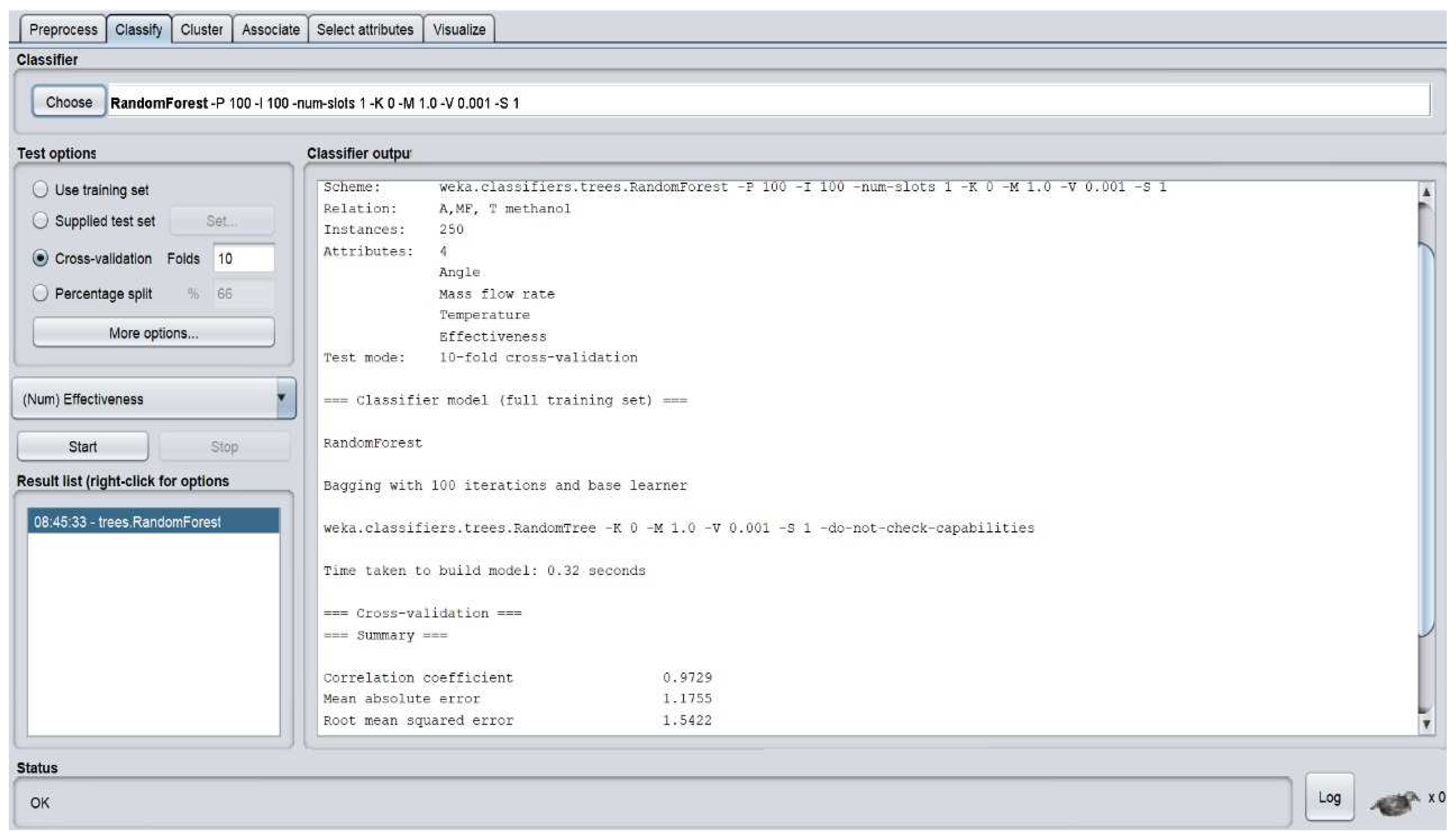
| 27 | RF | 1.1755 | 1.5422 |
| 28 | RT | 1.8456 | 2.4296 |
| 29 | REP TREE | 1.9963 | 2.5834 |
| 30 | IMC | 5.0530 | 6.1989 |
| Categories | SUBSETS | A | A-T | A-MF-T | Mean | ||||
|---|---|---|---|---|---|---|---|---|---|
| ALGORITHMS | MAE | RMSE | MAE | RMSE | MAE | RMSE | MAE | RMSE | |
| Functions | SLR | 4.972 | 6.139 | 4.456 | 5.660 | 4.456 | 5.660 | 4.628 | 5.820 |
| LR | 4.972 | 6.139 | 4.338 | 5.589 | 4.338 | 5.589 | 4.549 | 5.772 | |
| LMs | 4.974 | 6.421 | 4.301 | 6.044 | 4.266 | 5.991 | 4.514 | 6.152 | |
| MLP | 4.986 | 6.126 | 4.281 | 5.597 | 4.209 | 5.691 | 4.492 | 5.805 | |
| GP | 5.063 | 6.180 | 4.315 | 5.606 | 4.301 | 5.575 | 4.560 | 5.787 | |
| RBFN | 4.914 | 6.061 | 4.488 | 5.636 | 4.809 | 5.892 | 4.737 | 5.863 | |
| RBFR | 4.100 | 4.951 | 3.676 | 4.791 | 3.740 | 4.874 | 3.839 | 4.872 | |
| SMOREG | 4.983 | 6.248 | 4.240 | 5.789 | 4.204 | 5.758 | 4.476 | 5.931 | |
| IBK | 3.673 | 4.415 | 2.631 | 3.062 | 4.315 | 6.621 | 3.540 | 4.699 | |
| Kstar | 4.208 | 5.166 | 3.236 | 4.116 | 3.217 | 4.256 | 3.554 | 4.513 | |
| LWL | 3.900 | 4.691 | 3.336 | 4.259 | 3.506 | 4.487 | 3.581 | 4.479 | |
| Meta | AR | 3.728 | 4.475 | 2.373 | 2.921 | 1.631 | 2.089 | 2.577 | 3.161 |
| BREP | 3.701 | 4.458 | 2.498 | 2.935 | 1.598 | 2.099 | 2.599 | 3.164 | |
| MS | 5.053 | 6.199 | 5.053 | 6.199 | 5.053 | 6.199 | 5.053 | 6.199 | |
| RC | 3.673 | 4.415 | 2.631 | 3.062 | 1.325 | 1.705 | 2.543 | 3.061 | |
| RFC | 3.673 | 4.415 | 2.655 | 3.152 | 4.601 | 6.965 | 3.643 | 4.844 | |
| RSS | 3.707 | 4.446 | 3.331 | 4.175 | 2.511 | 3.102 | 3.183 | 3.908 | |
| RBD | 3.702 | 4.410 | 2.578 | 3.075 | 1.961 | 2.425 | 2.747 | 3.303 | |
| STACKING | 5.053 | 6.199 | 5.053 | 6.199 | 5.053 | 6.199 | 5.053 | 6.199 | |
| VOTE | 5.053 | 6.199 | 5.053 | 6.199 | 5.053 | 6.199 | 5.053 | 6.199 | |
| WIHW | 5.053 | 6.199 | 5.053 | 6.199 | 5.053 | 6.199 | 5.053 | 6.199 | |
| Rules | DT | 3.673 | 4.415 | 2.631 | 3.062 | 2.631 | 3.062 | 2.978 | 3.513 |
| M5R | 3.721 | 4.485 | 2.606 | 3.178 | 2.798 | 3.639 | 3.042 | 3.768 | |
| ZEROR | 5.053 | 6.199 | 5.053 | 6.199 | 5.053 | 6.199 | 5.053 | 6.199 | |
| Trees | DS | 4.567 | 5.613 | 4.152 | 5.317 | 4.152 | 5.317 | 4.290 | 5.415 |
| M5P | 3.843 | 4.632 | 2.927 | 3.666 | 2.944 | 3.752 | 3.238 | 4.017 | |
| RF | 3.671 | 4.417 | 2.627 | 3.052 | 1.176 | 1.542 | 2.491 | 3.004 | |
| RT | 3.673 | 4.415 | 2.631 | 3.062 | 1.846 | 2.430 | 2.717 | 3.302 | |
| REP TREE | 3.683 | 4.427 | 2.600 | 3.120 | 1.996 | 2.583 | 2.760 | 3.377 | |
| IMC | 5.053 | 6.199 | 5.053 | 6.199 | 5.053 | 6.199 | 5.053 | 6.199 | |
Publisher’s Note: MDPI stays neutral with regard to jurisdictional claims in published maps and institutional affiliations. |
© 2022 by the authors. Licensee MDPI, Basel, Switzerland. This article is an open access article distributed under the terms and conditions of the Creative Commons Attribution (CC BY) license (https://creativecommons.org/licenses/by/4.0/).
Share and Cite
Nair, A.; P., R.; Mahadevan, S.; Prakash, C.; Dixit, S.; Murali, G.; Vatin, N.I.; Epifantsev, K.; Kumar, K. Machine Learning for Prediction of Heat Pipe Effectiveness. Energies 2022, 15, 3276. https://doi.org/10.3390/en15093276
Nair A, P. R, Mahadevan S, Prakash C, Dixit S, Murali G, Vatin NI, Epifantsev K, Kumar K. Machine Learning for Prediction of Heat Pipe Effectiveness. Energies. 2022; 15(9):3276. https://doi.org/10.3390/en15093276
Chicago/Turabian StyleNair, Anish, Ramkumar P., Sivasubramanian Mahadevan, Chander Prakash, Saurav Dixit, Gunasekaran Murali, Nikolai Ivanovich Vatin, Kirill Epifantsev, and Kaushal Kumar. 2022. "Machine Learning for Prediction of Heat Pipe Effectiveness" Energies 15, no. 9: 3276. https://doi.org/10.3390/en15093276
APA StyleNair, A., P., R., Mahadevan, S., Prakash, C., Dixit, S., Murali, G., Vatin, N. I., Epifantsev, K., & Kumar, K. (2022). Machine Learning for Prediction of Heat Pipe Effectiveness. Energies, 15(9), 3276. https://doi.org/10.3390/en15093276