Article

A Galerkin Method for the Simulation of Laminar Boundary Layers on Heated Walls

ONERA/DMPE, Université de Toulouse, F-31055 Toulouse, France
*
Author to whom correspondence should be addressed.
Energies 2022, 15(9), 3267; https://doi.org/10.3390/en15093267
Submission received: 2 March 2022 / Revised: 21 April 2022 / Accepted: 27 April 2022 / Published: 29 April 2022
(This article belongs to the Special Issue Aerodynamics and Heat Transfer for Aircraft and Aerospace Systems)

Abstract

:
This paper presents a new solution method for the calculation of laminar thermal boundary layers. The method consists of a coupling between a modal method (Galerkin method) in the direction normal to the wall and a finite volume method in the direction(s) tangential to the wall. It is similar to an integral method in the sense that only a surface mesh is required and that the unknowns are integral quantities (corresponding to the moments up to a fixed order of the temperature profile in the direction normal to the wall). A specificity of the Galerkin method used is that the domain over which the integrals are computed has a variable size that is also an unknown of the problem. Using a series of numerical tests (representative of situations that can be encountered in aeronautics in the case of a wing equipped with a thermal ice protection system), we show that the new method allows us to predict the quantities of interest with a maximum error of a few percent, while a usual integral method (with only one unknown per mesh cell) is unable to treat the case of boundary layers on heated walls with a strong longitudinal temperature gradient, as shown in the literature.

1. Introduction

Although the resolution of thermal boundary layers most often relies on solving Navier–Stokes equations, there are still fields of application for which the pursuit of very fast methods of solving this problem is privileged. For instance, aircraft in-flight icing prediction is one field for which it has remained common practice to calculate convective heat transfer by coupling inviscid fluid and boundary layer codes. Indeed, for both certification and aircraft design, a large number of icing conditions must be calculated within a reasonable time. In addition, the calculation procedure is sequential and quasi-steady. As the ice grows, the shape of the airfoil or obstacle is updated. The flow needs to be systematically calculated around this updated shape. Therefore, many aerodynamic calculations may be necessary. The same issue is faced when modeling the activation of thermal ice protection systems (electro-thermal or bleed-air systems): the resolutions of the aerodynamics, of the heat transfer in the substrate of the protected feature and of the water runback and freezing over the protected surface have to be coupled. This also leads to a huge number of aerodynamic simulations. As a result, a robust and fast calculation method for convective heat transfer is interesting for in-flight icing applications. This is the case in 2D but even more so in 3D due to the large number of degrees of freedom.
Icing problems are characterized by a separation of time scales such that the transient state of the aerodynamic flow can be considered as infinitely fast compared to the ice-growth duration and to the time required to reach thermal equilibrium inside the protected airfoil. This justifies the aforementioned use of a sequential coupling of several solvers for the simulations of ice accretion. Steady-state solutions of the aerodynamic field, and especially of the boundary layer, are also wanted for the same reason. To do so, integral-boundary-layer methods are often used for ice-accretion simulations. Since the core of this paper is dedicated to the modeling of boundary layers over heated walls, it is worth mentioning that boundary-layer solvers are also widely used in the icing community for modeling thermal ice protection systems. For instance, simplified (algebraic) integral methods are used by Morency et al. [1], Al-Khalil et al. [2], Silva et al. [3], Wright [4] and Bu et al. [5]. There are issues of inaccuracy in using such simple approaches on heated walls, as mentioned by Morency et al. [6]. To overcome these issues, it is possible to improve the heated boundary-layer resolution by solving the Navier–Stokes equations, as proposed, for instance, by Croce et al. [7], Wright [4] or Bu et al. [8]. It is also possible to replace the integral boundary-layer solver with a solver of the Prandtl boundary-layer equations as performed at ONERA [9,10] with the solver CLICET [11], or by Morency [6]. The latter approach is consistent with the search for codes with low-CPU time consumption. However, for such an approach, the surface grid is not independent of the location of the stagnation point or separation line, which is a constraint for the ice-accretion-simulation workflow, especially in 3D. Additionally, no solution can be produced by such a solver beyond the separation of the boundary layer. Bayeux et al. [12] thus developed an integral-boundary-layer solver in order to solve the dynamic boundary layer (not the simplified algebraic equations), with the purpose of an easy enough extension to 3D solutions on any kind of unstructured grids [13]. The solver was used successfully for ice-accretion simulations by Radenac et al. [14]. The laminar thermal boundary layer was solved in a similar integral way in [15] under the assumption that the wall temperature is uniform. However, Harry et al. [16] showed that this basic one-equation thermal boundary-layer integral method fails at capturing the evolution of the wall temperature for severe wall-heating conditions. Difficulties arise especially for large variations in wall temperature, which is the actual situation for surfaces thermally protected against ice. Complex temperature profiles are indeed impossible to predict with the one-equation integral method.
One solution to this issue is to use a system of integral equations [16] (a multi-equation model) instead of the usual single-equation method so that history effects can be taken into account through additional degrees of freedom. As the technique proposed in this work for deriving additional equations is to use a Galerkin-type approximation in the direction normal to the wall, it is worth mentioning Graebel et al.’s article [17] concerning the use of such a method for the solution of the thermal boundary layer. Their paper addresses the resolution of both the dynamic and thermal steady-state, incompressible, laminar boundary layers in 2D. The velocity and temperature profiles in the direction normal to the wall are projected onto orthonormal bases of functions, based on Laguerre polynomials. The system of partial differential equations that governs the boundary-layer behavior then becomes a system of ordinary differential equations with respect to the streamwise coordinate. This system is solved by a so-called predictor–corrector approach. Additionally, specific functions are introduced by Graebel et al. in order to speed up the convergence of the resolution. However, it has to be mentioned that the solved system of equations is actually a reshaped set of equations after Falkner–Skan transformations, which are well-adapted to the 2D incompressible laminar regime. In addition, their approach was only validated on a test case where the wall temperature is constant.
The aim of the present paper is therefore to present and discuss a multi-equation method based on an integral approach for the solution of the steady-state energy equation in the boundary layer. The method has to be compliant with simulations of non-uniformly heated walls in order to be able to model the use of ice protection systems. As in Graebel et al.’s article [17], attention is limited to the 2D laminar flow regime that is important for icing applications, as the flow near the leading edge is generally laminar. However, it is required that the model should be compliant with future extensions to 3D configurations and to the turbulent regime (meaning that, for instance, no Falkner–Skan transformation has to be introduced). To meet these constraints, the classical boundary-layer energy equation is used to derive our system of integral equations by applying the Galerkin method with respect to the y-variable (normal direction to the wall). Since this equation is a scalar equation, with no specific 3D effects, the extension to 3D is expected to be straightforward. Contrary to Graebel et al.’s article [17], the solution of the sole energy equation in the boundary layer will thus be addressed. The solution of the dynamic boundary layer will be supposed to be known and given by another solver in a decoupled manner, which is suitable for incompressible flows. However, since a variable field of temperature in the boundary layer makes the density field variable too, the assumption of constant density will not be made in the derivation of the equations, and the impact of compressibility effects will be discussed. The method presented here is not limited to aircraft in-flight icing applications. In particular, since integral boundary layer methods have already been developed to study wind turbines [18], and these can also be thermally protected against icing [19], the method presented here can also be applied in this area. Integral boundary layer methods may also be used for aerodynamic design in the aeronautical industry [20] or for the modeling of wall mass transfers [21] (and more generally for the rapid design and optimization of any system involving heat and mass transfer induced by forced convection). Nevertheless, in the present work, the method will be tested in representative cases of icing applications only.
The paper is divided into four parts. The first part recalls the boundary-layer energy equation and the corresponding assumptions on which the proposed solution method is based (Section 2). The solution method is shown in Section 3. This is an original method where the evolution in the normal direction to the wall is discretized with a Galerkin method (yielding to a system of integral equations), whereas the streamwise evolution is discretized with the finite volume method. The basis of functions used with the Galerkin method is less optimized for laminar regime than Graebel et al.’s approach [17]. However, it should be possible to extend the method to the turbulent regime in the future (with several adjustments that are not discussed in this article). The last part of the article discusses the use of the proposed method on test cases representative of in-flight icing conditions, especially with non-uniform wall temperature, which are rarely addressed with integral methods in the literature (Section 4).

2. Laminar Boundary-Layer Energy Equation

The goal of this work is to solve an energy equation for the 2D compressible laminar boundary layer, assuming that the flow is steady outside of the boundary layer. The major point of the compressible assumption is to allow the density to be variable, which is mainly due to the dilatability in the case treated here.
Let us consider the variation in the enthalpy h ( t , x , y ) as a function of time (t) and position in a 2D boundary layer, where x is the streamwise direction and y is the direction normal to the wall. The equation reads [22]:
ρ t h + ρ u x x h + ρ u y y h = t p + u x x p y ϕ + D ˙
where ρ ( t , x , y ) is the density, u x ( t , x , y ) and u y ( t , x , y ) are the flow velocities in the x and y direction, respectively, and p ( t , x , y ) is the pressure. Moreover, the heat flux reads:
ϕ = k y T
where T ( t , x , y ) is the temperature and k is the thermal conductivity of the fluid (generally a function of T). Finally, the viscous dissipation reads:
D ˙ = τ x y y u x
The viscous shear stress is τ x y = μ y u x , where μ is the dynamic viscosity of the fluid (also depending on T in general).
Additionally, it is worth recalling that the other equations governing the 2D compressible laminar boundary layer are as follows [22]:
t ρ + x ρ u x + y ρ u y = 0
ρ t u x + ρ u x x u x + ρ u y y u x = x p + y τ x y
y p = 0
Equation (4) is the continuity equation, while Equations (5) and (6) are the momentum equations in the streamwise and normal directions, respectively.
For the numerical integration presented in Section 3, it is of practical interest to derive an equivalent equation for the thermal boundary layer by replacing T with a new unknown θ ( t , x , y ) = T e ( x ) T ( t , x , y ) , which by definition vanishes at the edge of the boundary layer (where the temperature is T e ). It is worth noticing that the temperature T e depends only on x, as do the other variables at the edge of the boundary layer, pressure p e and velocity u x e , because a steady state is assumed and x is the streamwise direction.
First, the following equation for T is derived from Equation (1):
ρ c p t T + ρ c p u x x T + ρ c p u y y T = u x d x p e + y k y T + D ˙ ,
which stems from the fact that the specific heat capacity at a constant pressure is c p = T h p . This equation also accounts for the fact that Equation (6) implies that p ( t , x , y ) = p e ( x ) .
Equation (4) allows to further reshape Equation (7):
c p t ρ T + c p x ρ u x T + c p y ρ u y T = u x d x p e + y k y T + D ˙
Since the temperature T e ( x ) at the edge of the boundary layer depends only on x, the following equation on T T e = θ is obtained by simply subtracting T e × Equation (4) from Equation (8).
c p t ρ ( T T e ) + c p x ρ u x ( T T e ) + c p y ρ u y ( T T e ) + c p ρ u x d x T e = u x d x p e + y k y T T e + D ˙
The terms linked to the derivatives of p e and T e can be further simplified because the flow outside of the boundary layer is assumed to be inviscid and steady. Under these assumptions, the x-momentum equation of the system of Euler equations simply reads:
ρ e u x e d x u x e = d x p e
Considering that the total enthalpy h i , e outside of the boundary layer is constant, it can also be stated that:
d x h i , e = 0 = c p e d x T e + 1 2 d x u x e 2
Finally, Equations (10) and (11) imply that:
d x p e = ρ e 2 d x u x e 2 = ρ e c p e d x T e
Consequently, Equation (9) writes:
c p t ρ θ + c p x ρ u x θ + c p y ρ u y θ = ρ c p ρ e c p e u x d x T e + y k y θ D ˙
Eventually, if the specific heat capacity is assumed constant, which is a fairly good assumption for air in the relatively narrow range of temperatures investigated in the field of icing (around 223 K to 373 K), the equation governing the relative temperature θ in the boundary layer reads:
t ρ c p θ + x ρ u x c p θ + y ρ u y c p θ = ρ ρ e c p u x d x T e + y k y θ D ˙
Although Equation (14) is unsteady, it will be used to build an iterative numerical method that converges towards the steady-state solution. This method is easy to generalize in 3D and on any surfaces. More specifically, the equation that will be solved for this purpose is the following one:
t ρ e c p θ + x ρ u x c p θ + y ρ u y c p θ = ρ ρ e c p u x d x T e + y k y θ D ˙ .
Using a density independent of y in the time derivative does not affect the steady-state solution and will simplify the resolution.
There is no major difficulty in deriving the equation for the 3D case, where a crosswise z direction must be defined (the only additional assumption is that of irrotationality of the edge flow). Equation (15) is simply replaced by:
t ρ e c p θ + x ρ u x c p θ + y ρ u y c p θ + z ρ u z c p θ = ρ ρ e c p u x x T e + u z z T e + y k y θ D ˙

3. Solution Method

The solution method proposed here is a hybrid method of Galerkin type with respect to the y variable and of finite volume type with respect to the other space variables x and z. It has the advantage of requiring only a 2D surface mesh (in 3D) or a 1D linear mesh (in 2D), which not only reduces the computational cost but also greatly simplifies the implementation of the method. Indeed, in practice, the same situation as in the case of an integral method is faced, with the difference that a system of integral equations must be solved (with a dimension depending on the order of the Galerkin method) instead of a single equation for the integral thickness of the boundary layer. In the following, in order to simplify the notations, the method will be presented in the 2D case, but its generalization in 3D does not present any theoretical difficulty.

3.1. Galerkin Method with Respect to the y Variable

The Galerkin method consists of searching for an approximation of the solution θ ( t , x , y ) of the following form:
θ ˜ ( t , x , y ) = def j = 1 N θ j ( t , x ) φ j ( y δ T ( t , x ) )
where δ T denotes the thickness of the thermal boundary layer, θ j are the modal coordinates (all having the dimension of a temperature) and the φ j are the basis functions defined as:
φ j ( y ^ ) = π j ( y ^ ) ( 1 y ^ ) q if y ^ [ 0 , 1 ] , φ j ( y ^ ) = 0 if y ^ [ 1 , + ] ,
where y ^ = y δ T , q is a strictly positive constant and π 1 , , π N are N independent polynomials, whose expressions will be specified later (the degree of π j is less than or equal to j). It is worth mentioning that the approximate solution θ ˜ ( t , x , y ) satisfies by construction the boundary condition θ ( t , x , δ T ( t , x ) ) = 0 . As N increases, θ ˜ is a polynomial of increasingly higher degree in y and thus tends to oscillate in the vicinity of y = δ T . However, since the integer part of q 1 corresponds to the number of zero derivatives of θ ˜ at y = δ T , q allows us to control the behaviour of the solution in the vicinity of the boundary layer edge. At fixed N, if q is large enough, the oscillations can be suppressed, but if q is too high, the solution tends to flatten in the neighborhood of y = δ T , which leads to a decrease in the accuracy of the method. After various numerical tests, the choice q = m a x ( 2 , N ) appeared to be a good compromise and this value was thus adopted for all the numerical tests, which will be presented later in the paper.
From Equations (17) and (18), it appears that, at fixed t and x, the approximate solution θ ˜ is determined by N + 1 independent parameters, the modal coordinates θ 1 , , θ N and the thermal boundary layer (approximate) thickness δ T . One of these degrees of freedom can be easily removed. Indeed, using the Dirichlet boundary condition, θ = θ w = def T e T w in y = 0 , the following relationship is obtained:
j = 1 N θ j φ j ( 0 ) = θ w
Hence, if the π j polynomials are chosen such that π 1 ( 0 ) = 1 and π j ( 0 ) = 0 for j > 1 , this equation greatly simplifies:
θ 1 = θ w
The N unknowns of the problem are thus finally θ 2 , , θ N , δ T , and N independent equations must now be derived from the master Equation (15). To do this, Equation (15) just needs to be projected onto the space P N 1 of polynomials in y of degree less than or equal to N 1 . The solution of Equation (15) must therefore verify:
P P N 1 , 0 + [ t ( ρ e c p θ ) + x ( ρ c p u x θ ) + y ( ρ c p u y θ ) y ( k y θ ) ( ρ ρ e ) c p u x x T e + D ˙ ] P ( y ) d y = 0
P N 1 is a vector space of dimension N; it suffices to take for P the N monomials ψ i defined by ψ i ( y ) = def C i y i 1 for i = 1 N , where the C i are normalization constants whose values will be specified later on. By replacing in Equation (21), the exact solution θ by the approximate solution θ ˜ and the polynomial P by each of the monomials ψ i , the following system of equations is obtained:
i = 1 N , t M i + x F x , i = S i
where by definition (the variables x and t being omitted for clarity):
M i = def ρ e c p 0 + θ ˜ ( y ) ψ i ( y ) d y
F x , i = def 0 + ρ ( y ) c p u x ( y ) θ ˜ ( y ) ψ i ( y ) d y
S i = def 0 + ψ i ( y ) y ( k y θ ˜ ) ( y ) d y 0 + y ( ρ c p u y θ ˜ ) ( y ) ψ i ( y ) d y + c p x T e 0 + ( ρ ( y ) ρ e ) u x ( y ) ψ i ( y ) d y 0 + D ˙ ( y ) ψ i ( y ) d y
It can be seen that the application of the Galerkin’s method with respect to the variable y leads to a system of conservation laws whose unknowns are the first N moments of the temperature profile (up to a multiplicative constant) and whose terms F x , i and S i correspond respectively to the convective fluxes in the x direction and to the source terms. The physical meaning of the different terms composing S i will be discussed later on.
For the system (22) to be mathematically well-posed, the relation between the moments M i ( i = 1 N ) and the temperature profile θ ˜ must be bijective so that the terms F x , i and S i can be considered as implicit functions of the moments. The necessity of this condition will become clear in the next subsection dedicated to the finite volume discretization of the system (22). One must therefore address the question of the computation of θ j for j = 1 N and δ T from the first N moments of θ ˜ , i.e., the question of the inversion of the system corresponding to Equation (23) for i varying from 1 to N. For this purpose, using the expression of θ ˜ , Equation (23) can be rewritten in the following matrix form:
M i = i = 1 N A i j ( δ T ) θ j
where the coefficients of the matrix A i j ( δ T ) are given by:
A i j ( δ T ) = def 0 + ρ e c p φ j ( y δ T ) ψ i ( y ) d y = C i δ T i ρ e c p 0 1 π j ( y ^ ) ( 1 y ^ ) q y ^ i 1 d y ^
From the point of view of the finite volume discretization of system (22), which will be exposed in the following section, the computation of δ T and of the θ j from the M i needs to be simple and always possible. For this, it is possible to play on the choice of the polynomials π j . Let us set by definition:
π j ( y ^ ) = B j 0 y ^ 0 + B j 1 y ^ 1 + B j 2 y ^ 2 + + B j j y ^ j
For the polynomial of the lowest degree, π 1 , it is natural to take a constant polynomial and thus to set π 1 1 (since all polynomials can be normalized arbitrarily). For the other polynomials ( j > 1 ), it was shown that it is necessary to have π j ( 0 ) = 0 to obtain the simple relation θ 1 = θ w . So, for all j = 2 N , the polynomials π j read:
π j ( y ^ ) = B j 1 y ^ 1 + B j 2 y ^ 2 + + B j j y ^ j
At fixed j, j conditions have to be imposed in order to fix the values of the coefficients B j k . We have chosen to impose that the matrix A i j is lower triangular (which ensures the possibility to inverse the system (26)) and that its diagonal terms verify the normalization condition A i i = δ T i ρ e c p . At fixed j, this leads to the following linear system of unknowns ( B j k ) k = 1 j :
k = 1 j 0 1 ( 1 y ^ ) q y ^ i 1 + k d y ^ B j k = 0 , i = 1 , , j 1 , k = 1 j 0 1 ( 1 y ^ ) q y ^ j 1 + k d y ^ B j k = 1 C j
The coefficients of this system Π i k = 0 1 ( 1 y ^ ) q y ^ i 1 + k d y ^ can be easily calculated by recurrence, leading to:
Π i k = q ! ( k + i 1 ) ! ( q + k + i ) !
At a fixed k, they are all the smaller as q and i are large. To make sure that all the B j k are of the same order of magnitude whatever the value of j between 2 and N, we have chosen to set:
C j = 0 1 ( 1 y ^ ) q y ^ j 1 d y ^ 1 = ( q + j ) ! q ! ( j 1 ) !
It is worth noticing that at the continuous level (or if a computer of infinite precision is used for the computations), the choice of C i has no incidence on the values of the approximated solution θ ˜ since only the products θ j π j play a role. The larger π j is, the smaller θ j is. The normalization is only important in finite precision because it avoids a too-large disparity between the θ j and thus allows a better conditioning of the problem.
For all j = 2 N , the system (30) can be solved analytically, but this is not useful as its numerical solution is very fast and does not present any difficulties (except for large j since the system then becomes ill-conditioned). In practice, the system (30) is solved numerically once and for all when the solver is launched and the values of N and q are fixed.
Let us now return to the problem of computing δ T and θ i , knowing the M i . It has already been determined that θ 1 = θ w . In addition, since by construction A 1 j = 0 for all j > 1 , the first equation of system (26) implies:
M 1 = A 11 θ 1
with:
A 11 = C 1 δ T ρ e c p 0 1 ( 1 y ^ ) q d y ^ = δ T ρ e c p
Hence:
δ T = M 1 ρ e c p θ w
δ T being known thanks to Equation (35) and the matrix A i j being lower triangular, the computation of the θ i for i = 2 N is then straightforward.
Finally, let us give some details on the physical meaning and the computation of the source terms S i ( i = 1 N ), which are actually composed of four terms according to Equation (25). The first term of S i :
Φ i ( θ ˜ ) = def 0 + ψ i ( y ) y ( k y θ ˜ ) ( y ) d y
accounts for the effect of the conductive heat transport in the y direction. Integrating by part and using the expression of θ ˜ , it can be rewritten as:
Φ i ( θ ˜ ) = j = 1 N θ j 0 + k δ T ψ i ( y ) φ j y δ T d y j = 1 N θ j k ( 0 ) δ T φ j ( 0 ) ψ i ( 0 )
which leads to:
Φ 1 ( θ ˜ ) = k ( 0 ) C 1 δ T 1 j = 1 N θ j φ j ( 0 ) i = 1 Φ i ( θ ˜ ) = C i ( i 1 ) δ T i 2 j = 1 N θ j 0 1 k ( y ^ ) y ^ i 2 φ j ( y ^ ) d y ^ i = 2 N
which can also be written in the following matrix form:
Φ i ( θ ˜ ) = j = 1 N K i j ( θ ˜ ) θ j
The second term of S i :
G i ( θ ˜ ) = 0 + y ( ρ c p u y θ ˜ ) ( y ) ψ i ( y ) d y
corresponds to the convective heat flux in the y direction. Performing an integration by part, the term G i reads:
G i ( θ ˜ ) = ( i 1 ) C i 0 + ρ ( y ) c p u y ( y ) θ ˜ ( y ) y i 2 d y
The third term of S i :
R i ( θ ˜ ) = c p x T e 0 + ( ρ ( y ) ρ e ) u x ( y ) ψ i ( y ) d y
takes into account the influence of the density variations accross the boundary layer. In this equation and the previous one, the density profile is related to the temperature profile using the relation:
ρ ( y ) = p e r T ( y ) = p e r ( T e θ ˜ ( y ) )
Lastly, the fourth term of S i :
Q ˙ i = 0 + D ˙ ( y ) ψ i ( y ) d y
accounts for the heat production due to viscous forces.
It should be noted that for the extension to 3D, the only changes are the following. Equation (16) is used as the starting point for the analysis, instead of Equation (15). Consequently, the system to be solved becomes:
i = 1 N , t M i + x F x , i + z F z , i = S i
where there is a cross-wise component F z , i to the convective flux term:
F z , i = def 0 + ρ ( y ) c p u z ( y ) θ ˜ ( y ) ψ i ( y ) d y .
Only the third term of S i , R i , has to be modified to account for the edge–temperature gradient along the cross-wise direction:
R i ( θ ˜ ) = c p x T e 0 + ( ρ ( y ) ρ e ) u x ( y ) ψ i ( y ) d y + c p z T e 0 + ( ρ ( y ) ρ e ) u z ( y ) ψ i ( y ) d y .

3.2. Finite Volume Method with Respect to the x Variable

To simplify the notations it is useful to set:
M = M 1 M N ,   F = F x , 1 F x , N ,   S = S 1 S N ,   Θ = θ 1 θ N
With these notations, the system (22) can be rewritten in the following more compact form:
t M + x F ( Θ , δ T ) = S ( Θ , δ T )
The finite volume method and the explicit Euler scheme applied to Equation (42) lead to the following numerical scheme:
M i n + 1 = M i n Δ t Δ x i ( F i + 1 / 2 n F i 1 / 2 n ) + Δ t S i n
where by definition Δ t is the time step, M i n denotes the value of the discrete solution in the mesh cell C i = [ x i 1 / 2 , x i + 1 / 2 ] at time t n = n Δ t , Δ x i = x i + 1 / 2 x i 1 / 2 is the size of the cell C i , F i + 1 / 2 n is the numerical flux between the cells C i and C i + 1 on the time interval [ t n , t n + 1 ] , and S i n is the discrete value of the source term in the cell C i on the time interval [ t n , t n + 1 ] .
The way to calculate the numerical fluxes and the source terms remains to be specified. As our first objective was simply to verify the potential of our method, we only implemented very simple numerical schemes. On the one hand, an explicit time discretization scheme is used, and on the other hand an upwind first order scheme is applied for the computation of the numerical fluxes (by upwinding according to the sign of the velocity u x e ). We have thus taken:
F i + 1 / 2 n = F ( Θ i n , δ T i n , u x e ( x i + 1 / 2 ) ) if u x e ( x i + 1 / 2 ) > 0 F i + 1 / 2 n = F ( Θ i + 1 n , δ T i + 1 n , u x e ( x i + 1 / 2 ) ) if u x e ( x i + 1 / 2 ) 0 ,
where the edge velocity used for upwinding is u x e ( x i + 1 / 2 ) = u x e ( x i ) + u x e ( x i + 1 ) / 2 , and
S i n = S ( Θ i n , δ T i n )
As they only involve smooth functions, all the integrals contained in the expression of the numerical fluxes and source terms can be approximated by using a Gauss–Legendre quadrature formula with q nodes, which is exact when the function to be integrated is a polynomial of degree 2 q 1 . In practice, we used a formula with 2 N nodes where N is the number of modes of the Galerkin method. We verified through different tests that the integration error was negligible compared to the other approximation errors.
Finally, the proposed method of resolution comes down to the following algorithm:
  • Solution initialization: in each cell, set: δ T i 0 = δ D ( x i ) , where δ D is the dynamic boundary layer thickness and θ 1 i 0 = θ w , θ 2 i 0 = 0 , , θ N i 0 = 0 .
  • Time iteration: in each cell, knowing M i n from the previous time step compute first δ T i n and Θ i n by using Equations (35) and (26). Then, compute the numerical fluxes and the source terms using Gauss–Legendre quadrature formulas, and finally update the solution using the scheme (43).
  • End of the computation: Iterate until convergence to the steady state, i.e., until a given norm of the residual drops below a predefined threshold.
As the objective is only to compute the stationary solution, it is preferable to choose the largest possible time step to accelerate the convergence. However, with the algorithm being explicit, the maximum value of the (local) time step Δ t i is limited by a numerical stability criterion of the form:
Max | u x e , i | Δ t i Δ x i , 2 κ e N 2 ( q + 1 ) 2 Δ t i ( δ T i n ) 2 CFL m a x
where κ e is the edge value of the thermal diffusivity κ = def k ρ c p and CFL m a x is a numerical parameter that can be taken to be equal to 1 according to all our numerical experiments (in practice, CFL m a x = 0.9 was used for the simulations of this article). The first term | u x e , i | Δ t i Δ x i is related to the convective flux in the x direction, and the second term 2 κ e N 2 ( q + 1 ) 2 Δ t i ( δ T i n ) 2 is related to the heat diffusion source term. The presence of N 2 is due to the fact that the higher the number of modes, the smaller the characteristic diffusion length scale in the y direction, which behaves like δ T N ( q + 1 ) . It must be noted that δ T / ( q + 1 ) corresponds to the effective boundary layer thickness rather than δ T itself. It will indeed be demonstrated later on that, contrary to δ T , this parameter converges to a constant value when the number of modes N increases. Additionally, the factor 2 is caused by the very usual constraint of a Fourier number criterion being lower than 1 / 2 in explicit resolution of the heat equation. In future works, the constraint (46) can be easily overcome by using an implicit Euler scheme instead of the current explicit Euler scheme.
Regarding the extension to 3D, as the system to be solved is only slightly modified, the same finite-volume method can be used. A standard upwind numerical scheme for unstructured surface meshes will then naturally handle the two components of the convective flux identified earlier.

4. Results and Discussion

The modal method described in Section 3 has been implemented in a code called BLIM2D. Several test cases computed with BLIM2D will be discussed in this section in order to show the interest of the method.

4.1. Test Case Definition

In this paper, wedge air-flow test cases will be considered. Flat profiles are thus investigated, for which the edge velocity is simply u x e = K x m (Figure 1). K and m are two constants that have to be set. K allows us to change the Mach number of the test case, while m is linked to the pressure gradient (and to the angle of the wedge). As a reminder, the well-known Falkner–Skan solutions are the solutions of the wedge-flow dynamic boundary layer. The wedge-flow cases are interesting because they allow us to validate the proposed solution method for a large set of academic test cases that are representative of real conditions. For instance, m = 1 corresponds to the air flow in the vicinity of a stagnation point (wedge with an angle equal to π / 2 ), which is a key area for icing applications. It is indeed a laminar region where some ice deposition occurs and where thermal protection systems are usually installed and produce a high amount of heat. This explains the large number of cases with this value of m in the remainder of the article. Further downstream, the flow is accelerated, which can be modelled by wedge flows with m [ 0 , 1 ] , with m = 0 being the flat-plate condition with zero pressure gradient (and constant edge velocity). Further downstream, the flow is finally decelerated, which can be modelled with m < 0 wedge-flows.
The wall temperature will be set either constant or linearly varying. The zero-temperature-gradient cases are simple enough cases for a basic single-equation integral-boundary-layer method to produce a good solution [13,16]. However, some aspects regarding the numerical resolution will be specifically investigated in these cases. The expected numerical results will be discussed in Section 4.2.1 for conditions allowing self-similar temperature profiles (test-case 1 of Table 1, as discussed later). The grid convergence of the solution will be shown in Section 4.2.2. The convergence of the solution with the number N of modes will be shown in Section 4.2.3. In particular, the wall heat flux and the temperature profiles produced by BLIM2D will be analyzed.
Regarding the non-zero temperature-gradient cases (Section 4.4), they were chosen after some literature review. In an article by Papadakis et al. [23], the wall temperature was shown to evolve almost linearly in some cases, with temperature gradients close to −400 K/m. The wall temperature is thus warmer at the beginning of the geometry (physical stagnation point) than further downstream. Test case 4 is expected to model these conditions (Table 1). For numerical purposes, test cases where the temperature gradient is zero or positive (+400 K/m) are also considered (test cases 3 and 5, respectively).
For these cases, the solution will be compared against a numerical reference solution provided by the code CLICET [11], which is a quite widely used solver for boundary-layer modeling [9,10,24,25]. Indeed, CLICET directly solves the boundary layer equations (Prandtl equations), and especially Equation (1), by using a 2D mesh and a finite volume method. It should be noted that the velocity fields in the boundary layer are not strictly the same for the two codes. BLIM2D is fed with the integral boundary layer solution exposed in the article of Bayeux et al. [12] (see Appendix A for more information), whereas CLICET uses its own velocity field, which is solved jointly with the temperature field. CLICET’s velocity field can thus be affected by the low effects of compressibility and moderate effects of dilatability. This potential source of discrepancies between BLIM2D and CLICET will be addressed in Section 4.3. To be more specific, in BLIM2D, the streamwise velocity profile u x ( y ) is computed using the integral method described in Bayeux et al. [12], while the normal velocity profile is given by the following equation:
u y ( y ) = 0 y x u x ( y ) d y ,
under the assumption that the velocity field is incompressible (which is consistent with Bayeux’s model assumptions [12]). Bayeux’s velocity profile is defined for 0 y δ , where δ is the dynamic boundary-layer thickness produced by the dynamic-boundary-layer integral model [12]. For y > δ , the velocity profile is extended with u x = u x e .
It should be noted (see Appendix B) that the model has also been validated against an empirical relation for a non-uniform wall temperature.

4.2. Convergence of the Method

The convergence of the method is assessed by refining the finite-volume grid and by increasing the number of modes of the Galerkin method.
For both investigations, the edge-flow conditions are those of test-case 1 in Table 1: a stagnation point ( m = 1 ), with a low Mach number M = 0.01 at the end of the plate ( L = 0.25 m) and a constant wall temperature T w = 264.15 K. As in all the following sections, uniform grids are used for which the number of cells N x lies between 64 and 512.
The Mach number is very low as well as the difference between the wall temperature and the edge-flow temperature. The very low Mach number implies low dissipation in the boundary layer, whereas the low temperature difference produces low dilatation effects and almost constant density in the boundary layer. The dynamic boundary layer is thus expected to remain unaffected by the wall heating. Both effects are favorable conditions for the self-similar behavior of the thermal boundary layer.

4.2.1. Description of the Investigated Test Case

First of all, the input parameters of simulations are of various kinds: the physical conditions given in Table 1 (boundary conditions at the edge of the boundary layer and at the wall), the velocity field in the boundary layer and the numerical parameters N and N x . Regarding the velocity field inside the boundary layer (for N x = 256 ), Figure 2 confirms that the velocity field provided to BLIM2D is not exactly the same as the reference CLICET velocity profile, although the discrepancies are small.
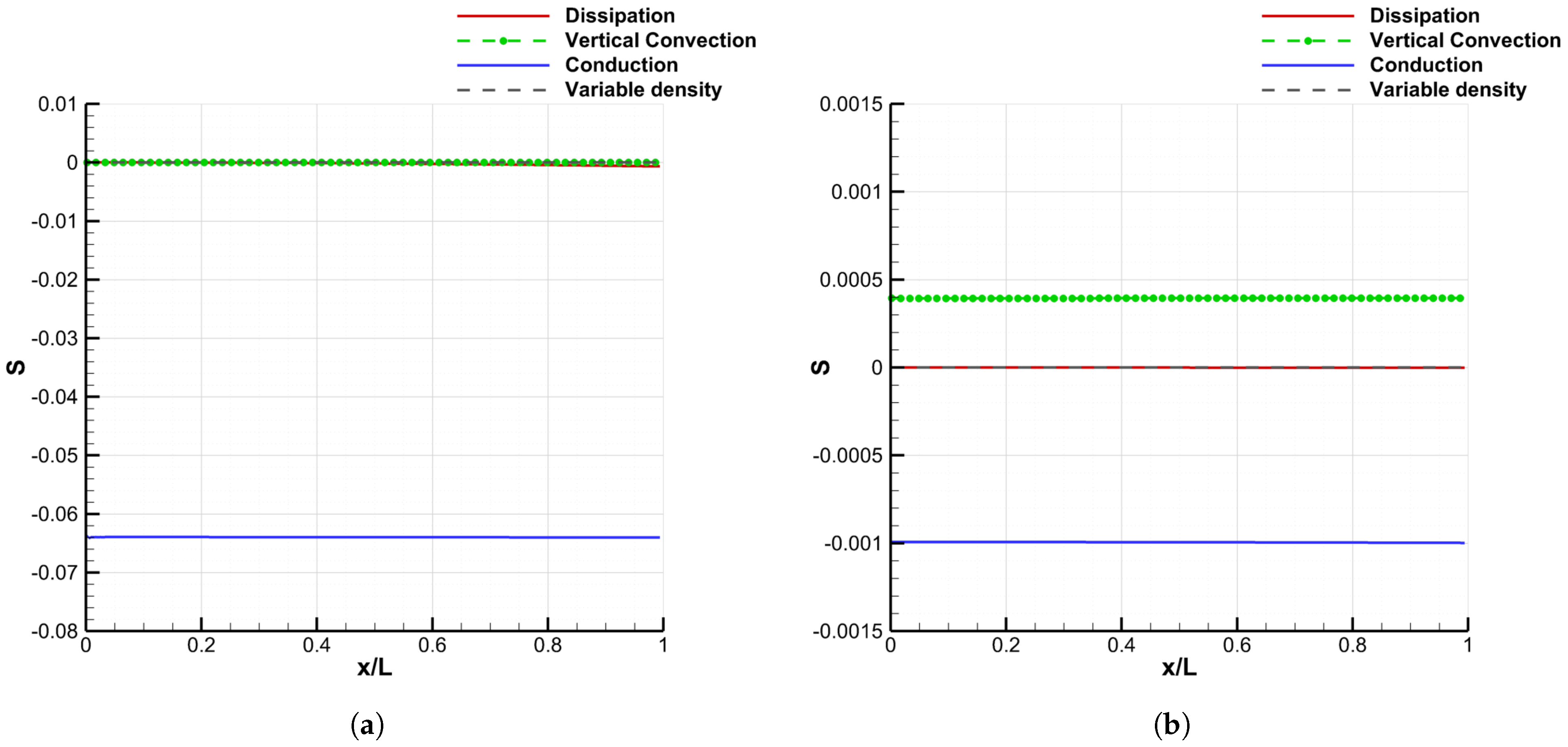
For N x = 256 and N = 5 , Figure 3a shows that for the first equation of system (22), the heat-flux source term Φ 1 is the only source term that does not vanish. For the second equation (Figure 3b), the dissipation Q ˙ 2 and density R 2 terms still vanish. The same behaviour is observed for the other equations, 3 to N (but it is not shown here for the sake of conciseness). This is consistent with the fact that the test-case running conditions were chosen so that dissipation is negligible and density varies little in order to achieve self-similar temperature profiles. It must be noted that the convective term G 2 is of the same order of magnitude as the heat flux term Φ 2 (although remaining lower). The same behavior is observed for the other equations, 3 to N (however, the source terms become lower for higher number of equations).
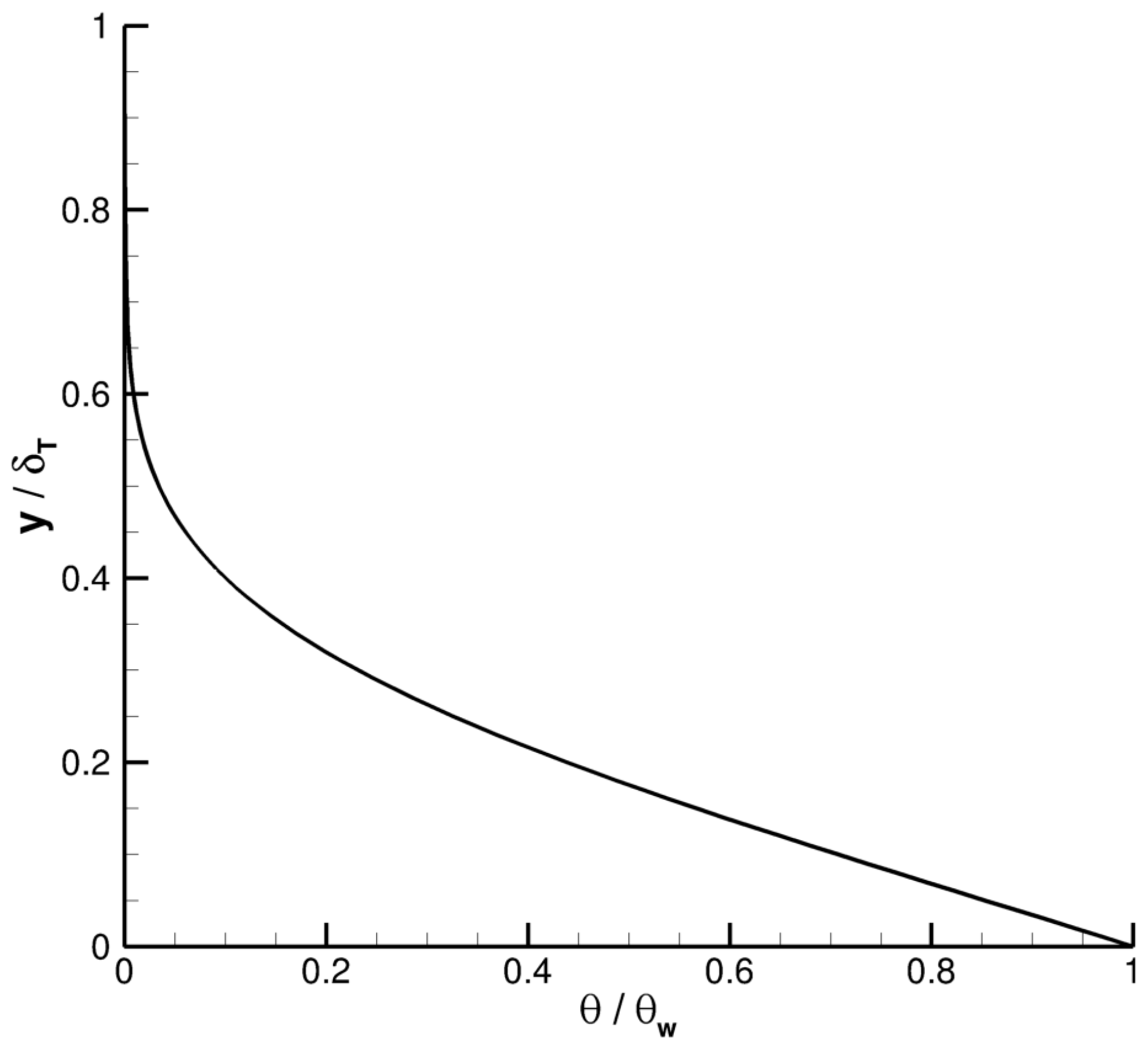
Figure 4 confirms that self-similar temperature profiles are produced by BLIM2D, and here for N = 4 : all the temperature profiles are superimposed at every point of the grid.

4.2.2. Grid Convergence

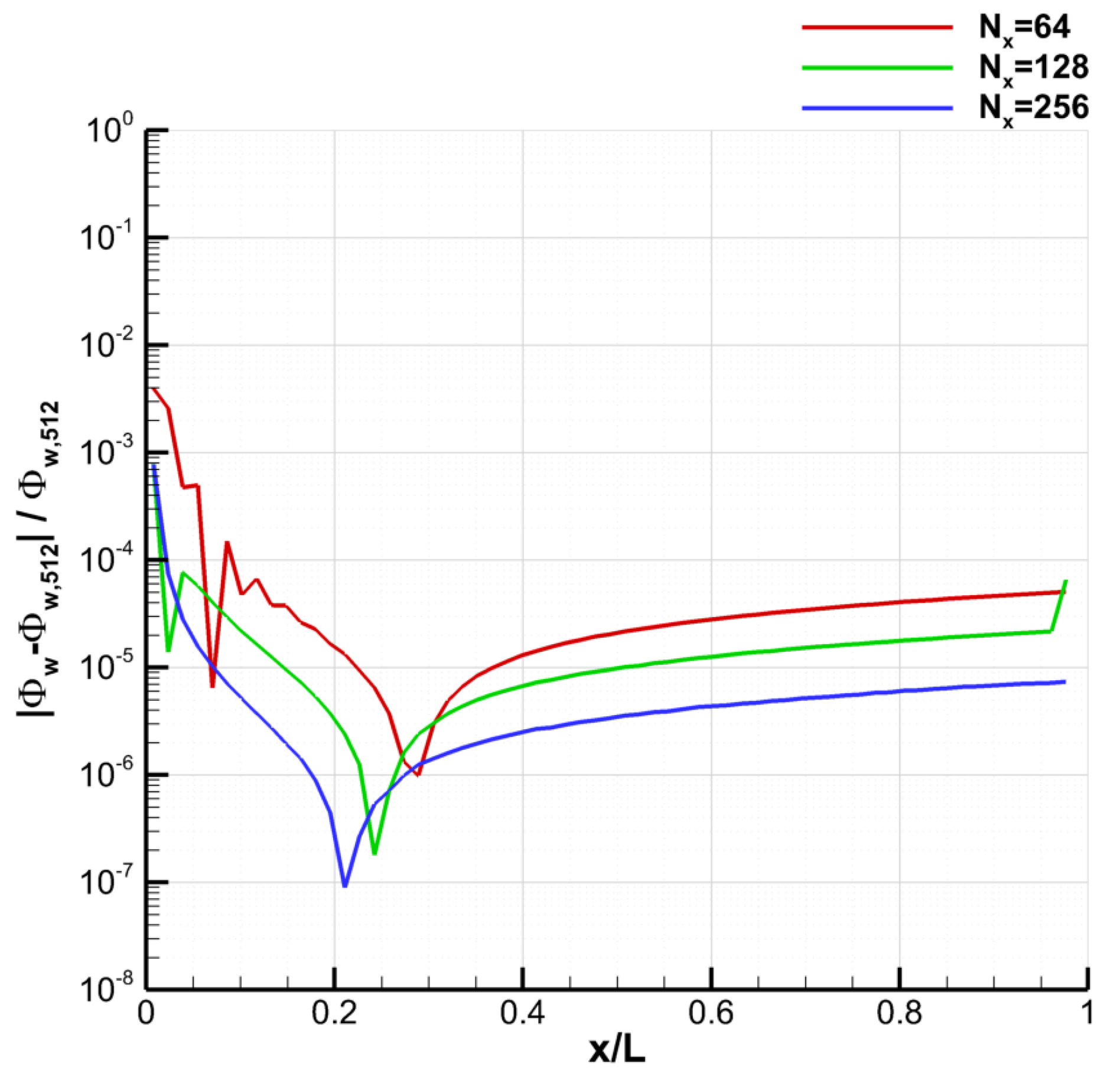
The finite volume method employed for the solution is not the most original part of this article. Therefore, this section only aims at showing that proper convergence is achieved when using refined surface grids. For a resolution with N = 4 equations, Figure 5 shows that the heat flux ϕ w is almost constant. There are some troubles in the vicinity of the inlet boundary condition at x / L = 0 . The results become smoother there for finer meshes. Otherwise, all mesh sizes N x { 64 , 128 , 256 , 512 } produce similar results. The computation of the relative error in the wall heat flux (compared to the finer mesh) shows that N x = 256 allows errors lower than 10 5 for x / L > 0.1 (Figure 6).

4.2.3. Convergence of the Galerkin Method

For the convergence of the Galerkin method, a uniform grid with N x = 256 points was used. The number of modes is increased from N = 1 to N = 5 to show the convergence. Since the Galerkin method is the core of this article, it is worth discussing several aspects of the solution that are affected by the number of modes employed.
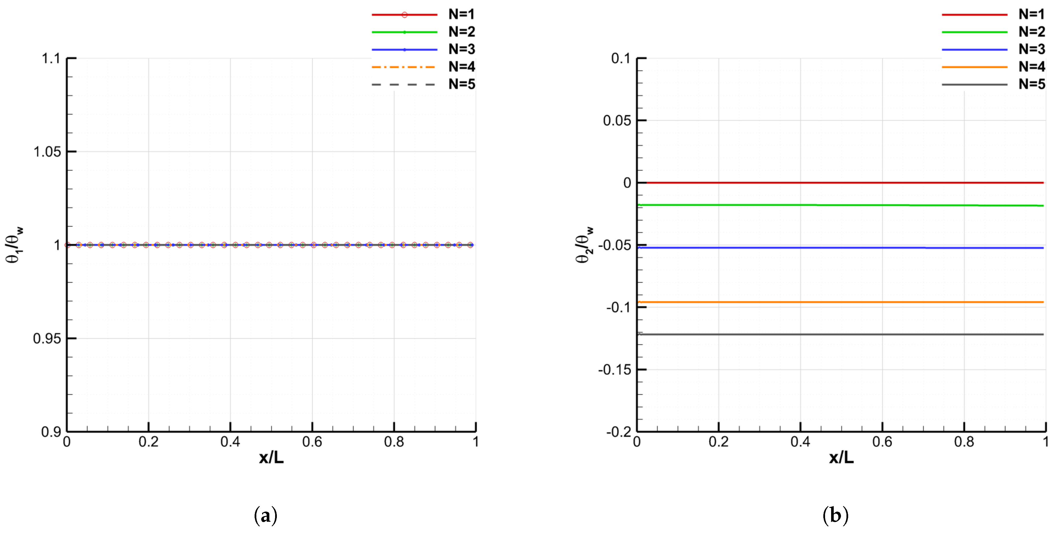
For the self-similar solution investigated here, where the temperature profiles are the same for all values of x, Equation (17) shows that the weights θ j are expected to be constant. Figure 7a shows θ 1 ,which is strictly equal to θ w as imposed by Equation (20). Another example is shown with θ 2 in Figure 7b. A constant value is obtained for all values of N (actually, a small variation of less than 1% is obtained), which indicates a good behavior of the solution. However, for a given j, the θ j values are not expected to converge when N increases. For instance, Figure 7b shows that | θ 2 | grows when N increases (obviously, θ 2 was set to 0 for N = 1 ). The same behavior was observed for θ 3 , θ 4 and θ 5 (the small variation can reach a few percent for θ 4 and θ 5 ), but it is not shown for the sake of conciseness. It must also be mentioned that, for a given value of N, the weights θ j tend to decrease when j increases. For instance, Figure 7a,b show that θ 1 is equal to θ w , whereas θ 2 / θ w is of the order of 10 2 to 10 1 . This reflects the fact that each additional mode contributes to the solution less and less strongly.
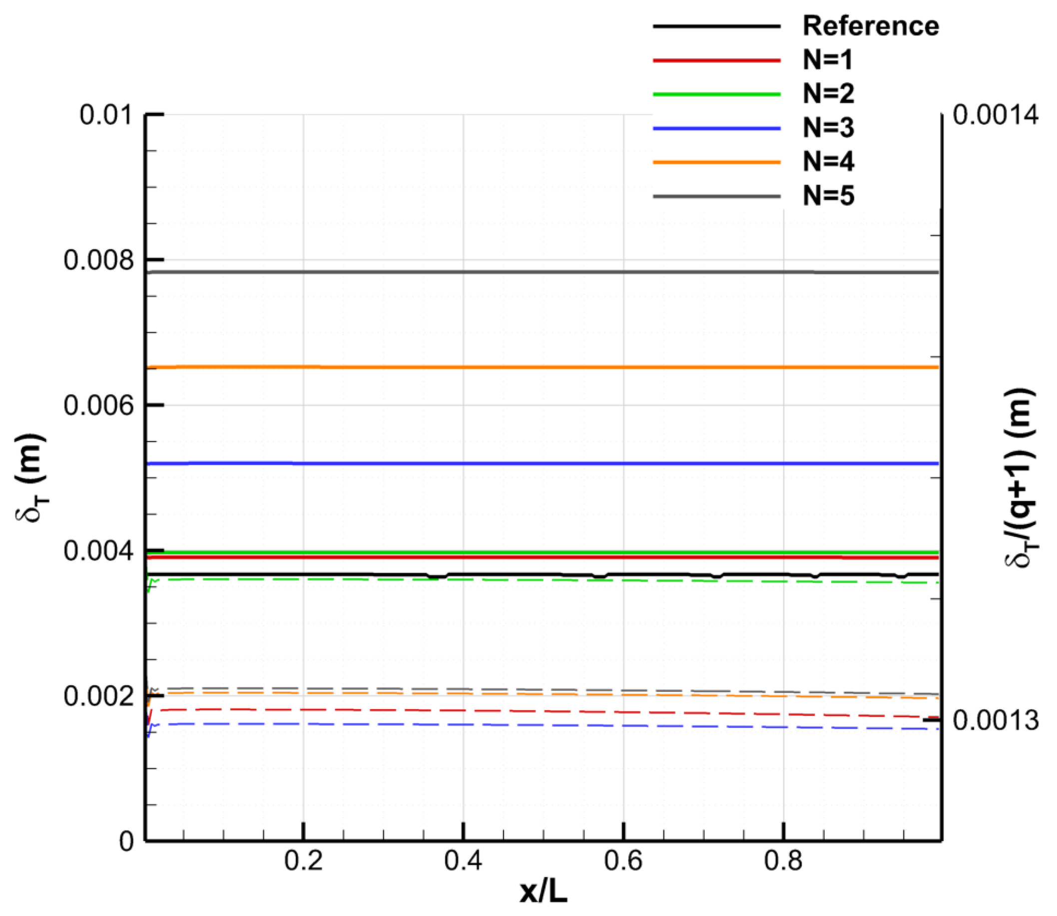
As explained in Section 3, the thermal-boundary-layer thickness δ T is an output of the numerical method. Figure 8 shows that it does not depend on x / L , which is consistent with the fact that the boundary layer thickness is constant for m = 1 [22]. The figure also demonstrates that δ T is not the same for all values of N. This is actually expected because Equation (35) implies that δ T is proportional to C 1 = q + 1 = m a x ( N + 1 , 3 ) via M 1 (for self-similar temperature profile and constant δ T ). δ T / ( q + 1 ) was thus also plotted in Figure 8 (dashed lines). A non-monotonic convergence is obtained for this parameter, which changes very little. The reference δ T in Figure 8 was provided by CLICET. The definition of δ T is actually not the same for CLICET (height at which θ reaches 0.01 × θ w ) and for BLIM2D (height at which the presumed temperature profile of Equation (17) reaches 0). In order to compare between the temperature profiles produced by CLICET and by BLIM2D, it is mandatory to define a common scale for the y coordinate. In the remainder of the article, this scale will be the thickness produced by CLICET, δ T , r e f .
Figure 9a shows the non-dimensional temperature profiles produced by BLIM2D for N = 1 to N = 5 modes, at x / L = 1 (the temperature profile is self-similar, so any value of x / L gives the same solution, except for small disturbances in the vicinity of x / L = 0 ). The agreement between the BLIM2D solutions and the reference solution is good, especially for N = 3 to N = 5 . To better quantify the errors in the BLIM2D solutions, three error norms defined as follows are plotted in Figure 9b. The L 1 norm is defined as:
ε L 1 = 2 L L / 2 L 1 δ T , r e f 0 δ T , r e f | θ ( x , y ) θ r e f ( x , y ) | d y d x ,
the L 2 norm is defined as:
ε L 2 = 2 L L / 2 L 1 δ T , r e f 0 δ T , r e f | θ ( x , y ) θ r e f ( x , y ) | 2 d y d x 0.5 ,
and the the L norm is defined as:
ε L = max x [ L / 2 , L ] max y [ 0 , δ T , r e f ] | θ ( x , y ) θ r e f ( x , y ) | .
For all three norms, the error decreases from N = 2 to N = 4 . N = 5 does not allow us to make the error drop further. It has to be noted that the L error is lower than 0.01 K, i.e., lower than 1% of the temperature difference between the wall and the edge of the boundary layer. This is really low for an error in temperature for icing applications.
The main output expected from BLIM2D is the wall heat flux, which can be made non-dimensional via the Stanton number:
S t = ϕ w ρ e u x e c p e ( θ w )
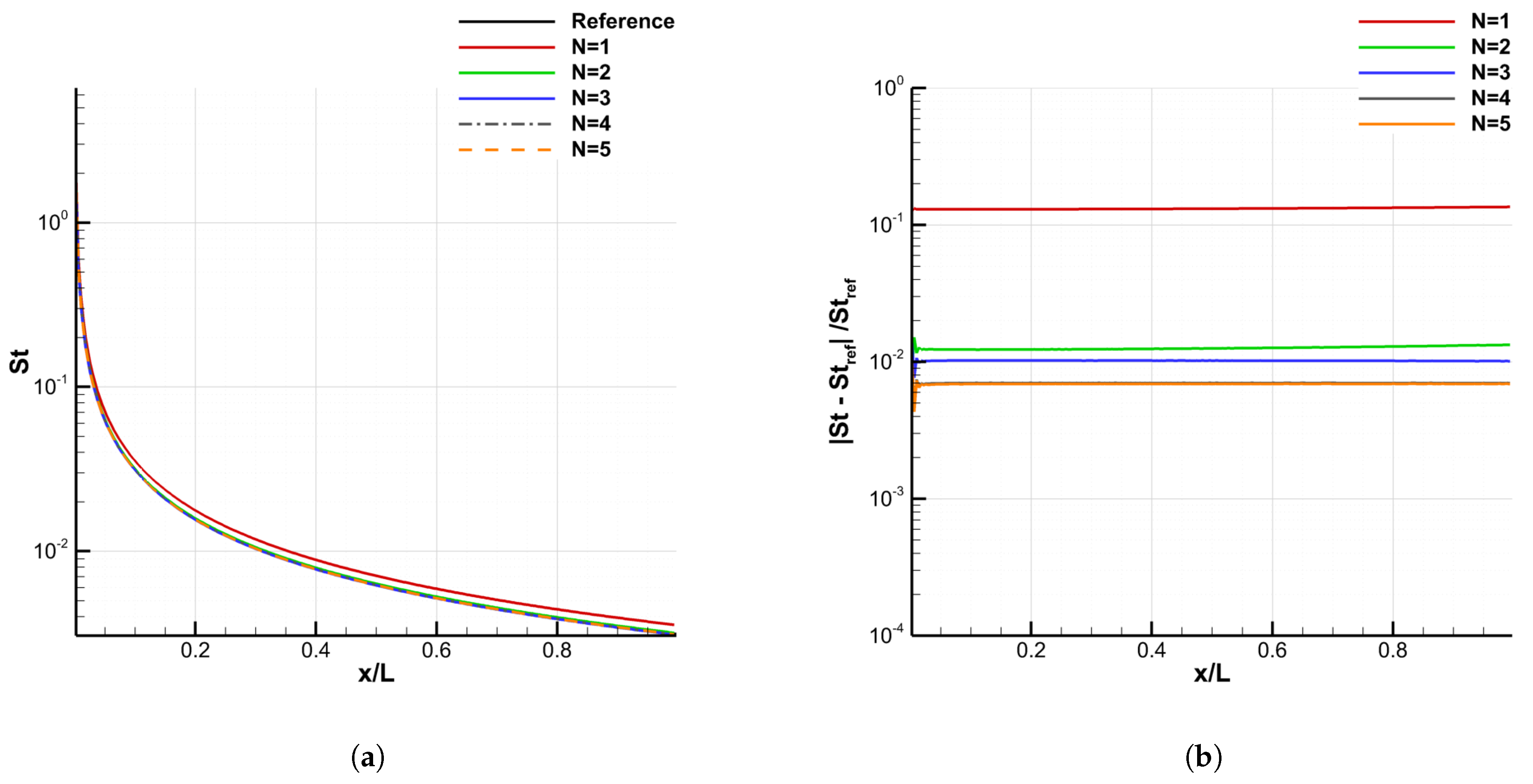
Figure 10a shows that the Stanton number is indeed little affected by N and the solution provided by BLIM2D is satisfactory. However, for this case, the Stanton number varies significantly because the heat flux ϕ w is almost constant and the velocity increases linearly from x = 0 to x = L . The relative error between the results produced by BLIM2D and CLICET shows that the modal approach also produces the lowest errors for N = 4 and N = 5 (Figure 10b). There is no significant difference between the errors for N = 4 and N = 5 , suggesting that the solution is converged for N = 4 . The relative error is around 7 × 10 3 . Again, regarding the targeted applications, this can be deemed as very low.
The main explanation for this residual error is that for this case, as mentioned earlier, the source term G i linked to the convection in the y direction cannot be neglected for Equations 2 to N (Equation (39)). Since the velocity fields are not exactly the same for CLICET and BLIM2D, the fact that G i is not negligible is a cause of the residual error in ϕ w : the use of the reference velocity field provided by CLICET in BLIM2D for u y allows us to decrease the relative error in S t to 4 × 10 3 . Additionally, an intrinsic source of error of the method is due to the definition used for the velocity profile u y for δ < y δ T . The use of Equation (47) with d x u x e 0 tends to arbitrarily extend u y linearly for y > δ . This does not make any real physical sense on the one hand, and on the other hand it introduces a difference with respect to CLICET, which has an evolution of u y bounded between y = 0 and the reference boundary-layer thickness δ T , r e f (as shown in Figure 2). This ultimately disturbs the calculation of the integral (39) for this case where δ < δ T .

4.3. Influence of the Wall to Free-Stream Temperature Ratio

In order to see the effect of the sole wall temperature on the solution (at fixed-edge temperature), the conditions of test case 2 were used (Table 1). These conditions are the same as test case 1, except that the edge-velocity exponent m can change and the wall temperature can be increased to values investigated in further test cases: T w 273.15 , 323.15 , 373.15 K (meaning that T w T e 10 , 60 , 110 K). The same grid was used as in Section 4.2.3, so N x = 256 .

4.3.1. Influence on the Velocity Profile

For m = 1 , Figure 11a shows that the higher the wall temperature, the higher the discrepancy between the reference velocity profile and the profiles used in BLIM2D that do not account for any effect of the temperature on the density changes.
It has to be noted that m = 1 provides a better overall agreement between BLIM2D and CLICET on the velocity profiles (even up to T w T e = 110 K) than any other value of pressure-gradient exponent m, as shown in Figure 11b. Less-accelerated ( m = 1 / 3 or m = 0 ) or decelerated flows ( m = 0.01961 ) exhibit larger L 2 relative errors in the velocity:
ε r , u x , L 2 = 2 L L / 2 L 1 δ r e f 0 δ r e f u x ( x , y ) u x r e f ( x , y ) u x r e f ( x , y ) 2 d y d x 0.5 , ε r , u y , L 2 = 2 L L / 2 L 1 δ r e f 0 δ r e f u y ( x , y ) u y r e f ( x , y ) u y r e f ( x , y ) 2 d y d x 0.5
Additionally, the errors tend to increase when T w T e is increased (except incidentally the error in u y for T w T e = 10 K). Finally, the relative error is larger in u y than in u x . However, while the relative error increases when m decreases for u x , there is no monotonic trend for the evolution of ε r , u y , L 2 with respect to m.

4.3.2. Consequences on the Wall Heat Flux

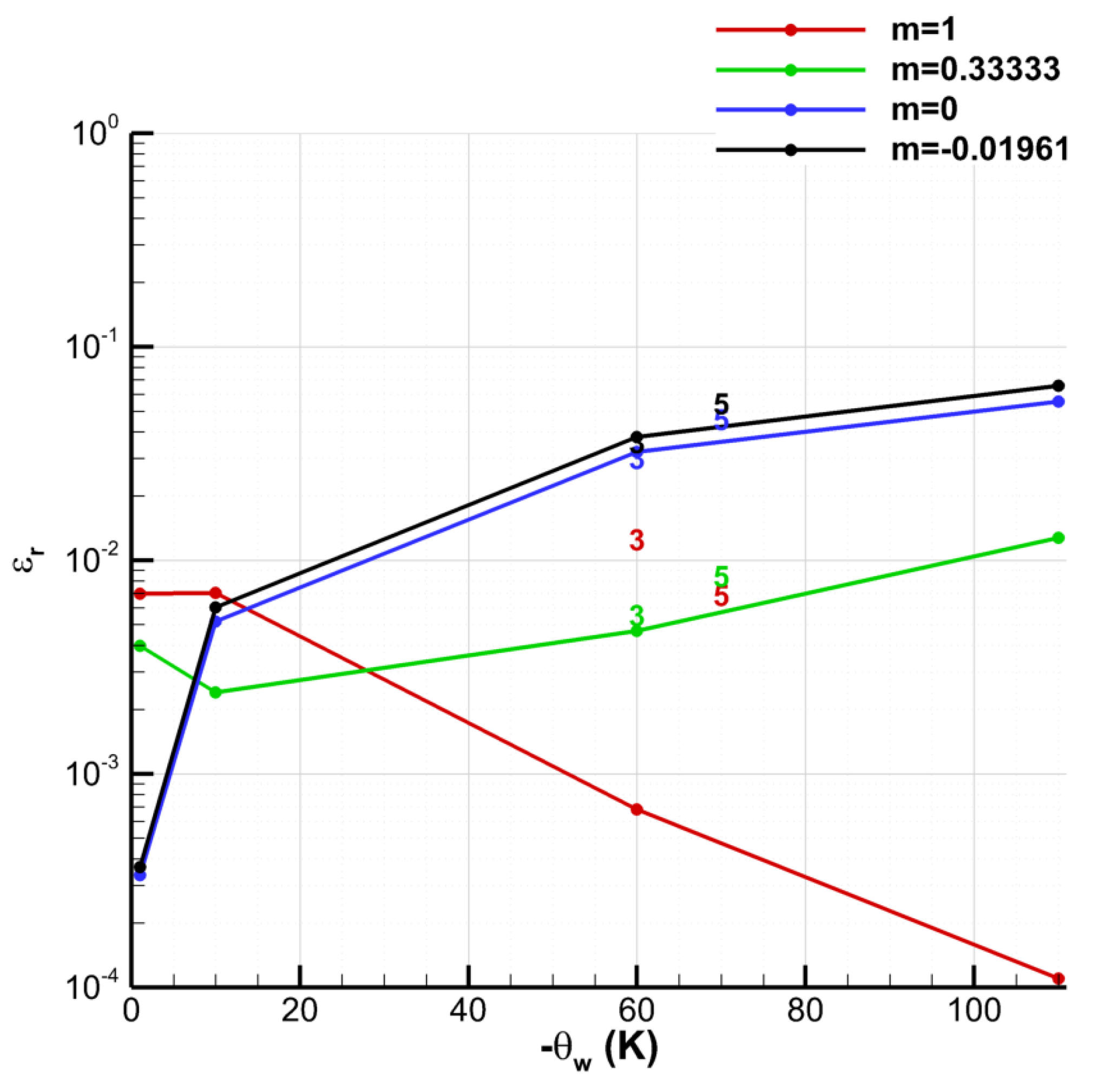
The error in the wall heat-flux prediction is shown in Figure 12 (for N = 4 ). Except for the stagnation point case m = 1 , the same trend is observed on the L 2 relative error
ε r , ϕ w , L 2 = 2 L L / 2 L ϕ w ( x ) ϕ w , r e f ( x ) ϕ w , r e f ( x ) 2 d x 0.5
as for the velocity profiles, the error increases when T w T e is increased. ε r , ϕ w , L 2 also tends to increase when m decreases. For the worst case, m = 0.01961 and θ w = 110 K, the relative error in the wall heat flux reaches 0.07 . So, the relative error remains moderate and is related to the errors in the input velocity profiles. Notice that for m = 1 , the relative error in the wall heat flux is even smaller: 7 × 10 3 for both θ w = 1 K and θ w = 10 K. However, it unexpectedly even drops lower than 10 3 for larger wall temperatures ( θ w = 60 K and θ w = 110 K). This surprising trend is attributed to the fact that the source term G i related to the convection in the y direction, which has an especially high contribution for m = 1 . Since, additionally, d x u x e has a higher value than for other values of m, as discussed earlier, the uncertainty is greater on the estimate of G i than for the other values of m.

4.4. Influence of the Wall Temperature Gradient

Test cases more representative of flight conditions are addressed in this section. In-flight icing often occurs for moderate Mach numbers. Here, the value M = 0.25 was retained. Several conditions of wall temperature are investigated (cases 3 with constant temperature, 4 with negative wall-temperature gradient and 5 with positive wall-temperature gradient, see Table 1). Additionally, the number of grid elements is still N x = 256 for all the simulations.
The relative errors in velocity profile of test cases 3, 4 and 5 are superimposed on the test case 2 curves in Figure 11b (test case numbers using a font color associated with the value of m). For the cases of non-zero gradient of temperature, the associated wall temperature is approximated, since it is not constant. The order of magnitude of the relative errors in the streamwise velocity is barely affected by the changed conditions. However, for the normal velocity, the error can be higher. In particular, the relative error can even largely exceed 100% for some cases: (1) where u y becomes low in a fairly extensive region near the wall ( m = 1 / 3 , T w · e x = 0 K/m), and (2) where the sign of u y changes along y ( m = 1 / 3 , T w · e x = 400 K/m; m = 0 or 0.1961 , T w · e x = −400 K/m).
Regarding the relative error in the wall heat flux, Figure 12 shows the errors for test cases 3, 4 and 5 in the same way as Figure 11b for the error in the velocity. The number of modes is N = 4 for all the solutions of this figure. The relative error exceeds 100% for test-case 4 because the heat flux changes sign, as shown later on. The relative error is thus very large in the area where the heat flux vanishes. Otherwise, the same orders of magnitude of error are retrieved as for the very low Mach number case 2. Moreover, the difficulties of the detailed analysis of the m = 1 case persist. The main conclusion is however that the relative error in heat flux does not exceed 7% for the cases investigated, which is mainly due to the errors in input–velocity profiles. This error is deemed reasonable for the envisioned applications.
In the remainder of this section, a more detailed analysis of the m = 1 and m = 0.01961 cases is made. Indeed, m = 1 is the stagnation-point condition, which is a key area for icing applications as already pointed out earlier. Moreover, the decelerated case m = 0.01961 exhibits the highest relative errors in heat flux.

4.4.1. Uniform Temperature, m = 1

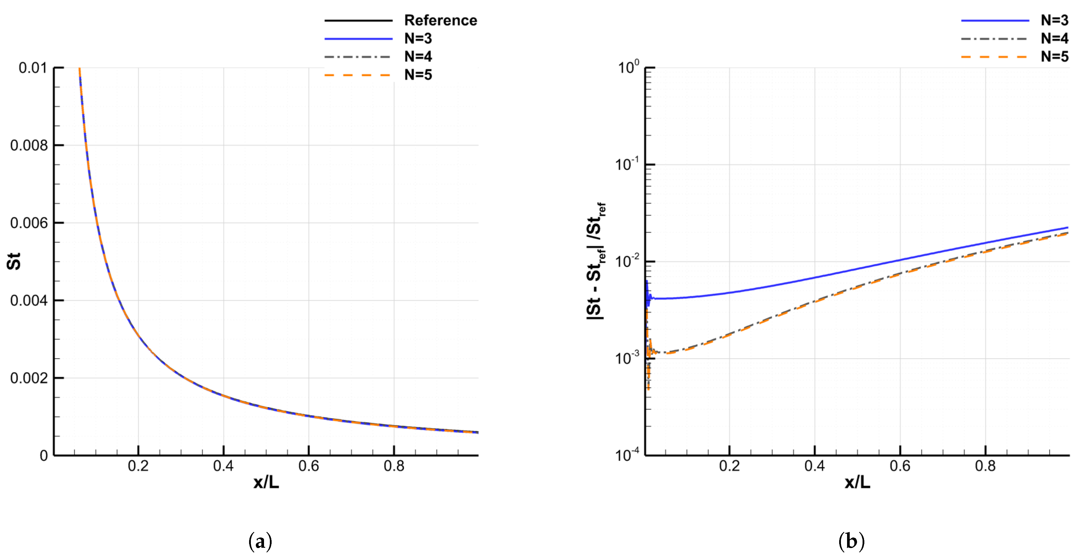
First, the test-case 3 with a constant wall temperature is investigated and N { 3 , 4 , 5 } . Figure 13 shows the Stanton number evolution as well as the relative error compared to the reference solution. The solution for N = 4 achieves convergence in a number of modes, similarly to the low Mach number condition investigated earlier. The relative error increases along the profile, reaching 2% for x / L = 1 . This is actually consistent with the fact that the error in the velocity was also observed to be increasing with x / L (which is not shown, for the sake of conciseness).
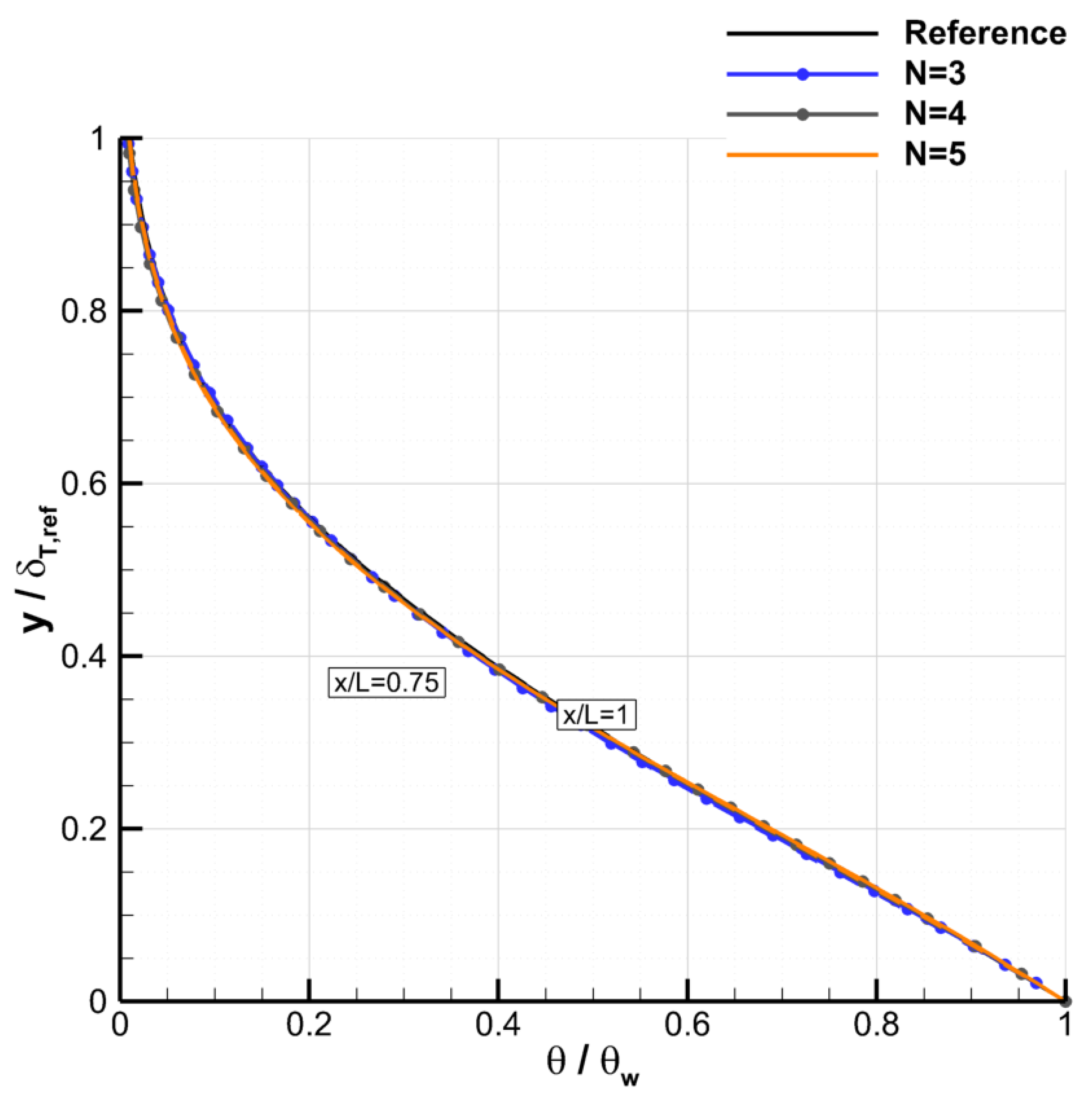
The solution is also good for the temperature profiles. The two temperature profiles shown in Figure 14 are very similar and the profiles produced by the various values of N are quite satisfactory.

4.4.2. Uniform Temperature Gradient −400 K/m, m = 1

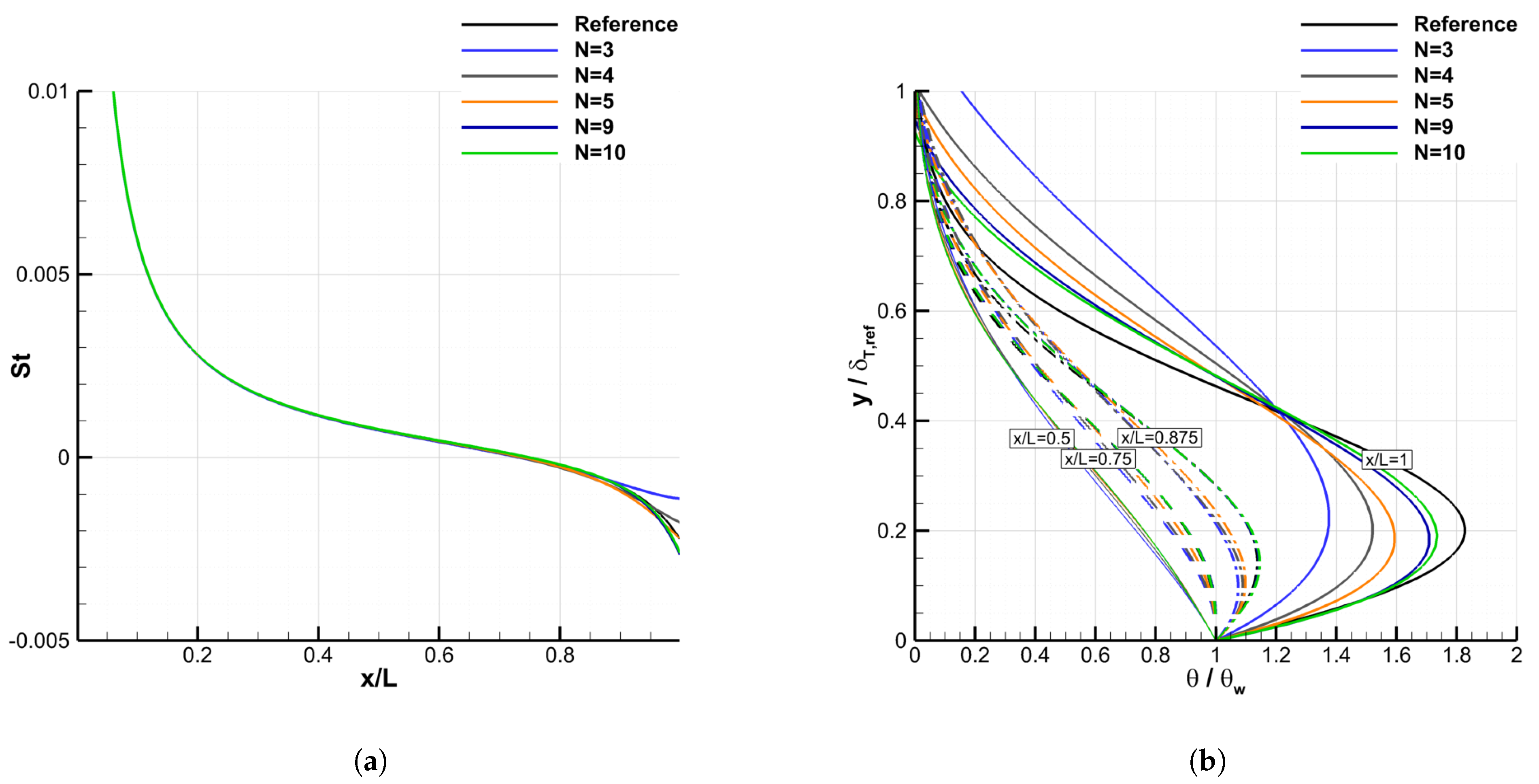
The negative wall temperature gradient test case is such that the wall temperature is 373.15 K for x / L = 0 and 273.15 K for x / L = 1. The wall heat flux is originally positive because the wall is warmer than the flow (and so is S t , Figure 15a). Nevertheless, since the wall is colder further downstream, the airflow eventually carries enough heat for the wall heat flux to change sign, around x c / L = 0.75 here. For x / L > x c / L , the wall actually cools the airflow. The area in the vicinity of x c / L is difficult to capture (the N = 3 curve starts departing from the reference curve there). Increasing N is extremely beneficial for capturing the whole trend further downstream.
The temperature profiles shown in Figure 15b are indeed not always monotonic ( x / L = 0.875 and x / L = 1 for instance). The heat transportation by the airflow actually heats the bottom part of the profile. This is more and more obvious for increasing values of x / L . This kind of profile is difficult to capture with temperature profiles in the form of Equation (17). Increasing the number of modes N allows higher-degree ( N + q ) polynomials for the modeling of the temperature profile. Convergence is thus achieved around N = 10 only and the trend of the reference profile is better captured with the highest values of N. This is also observed in x / L = 0.75 where the wall heat flux vanishes.
The error in the temperature profile increases at x / L = 1 . This is partly due to the fact that the error in the vertical velocity profile is larger at this location than upstream. This effect is even more pronounced because at this location, the vertical convection source term G has a greater relative importance in the overall balance. Moreover, the need to locally refine the mesh to follow the increasing gradient of the solution is not totally excluded. Despite this weakness, the reference solution is very well reproduced up to x / L = 0.875 and the error on the Stanton number remains acceptable.

4.4.3. Uniform Temperature Gradient +400 K/m, m = 1

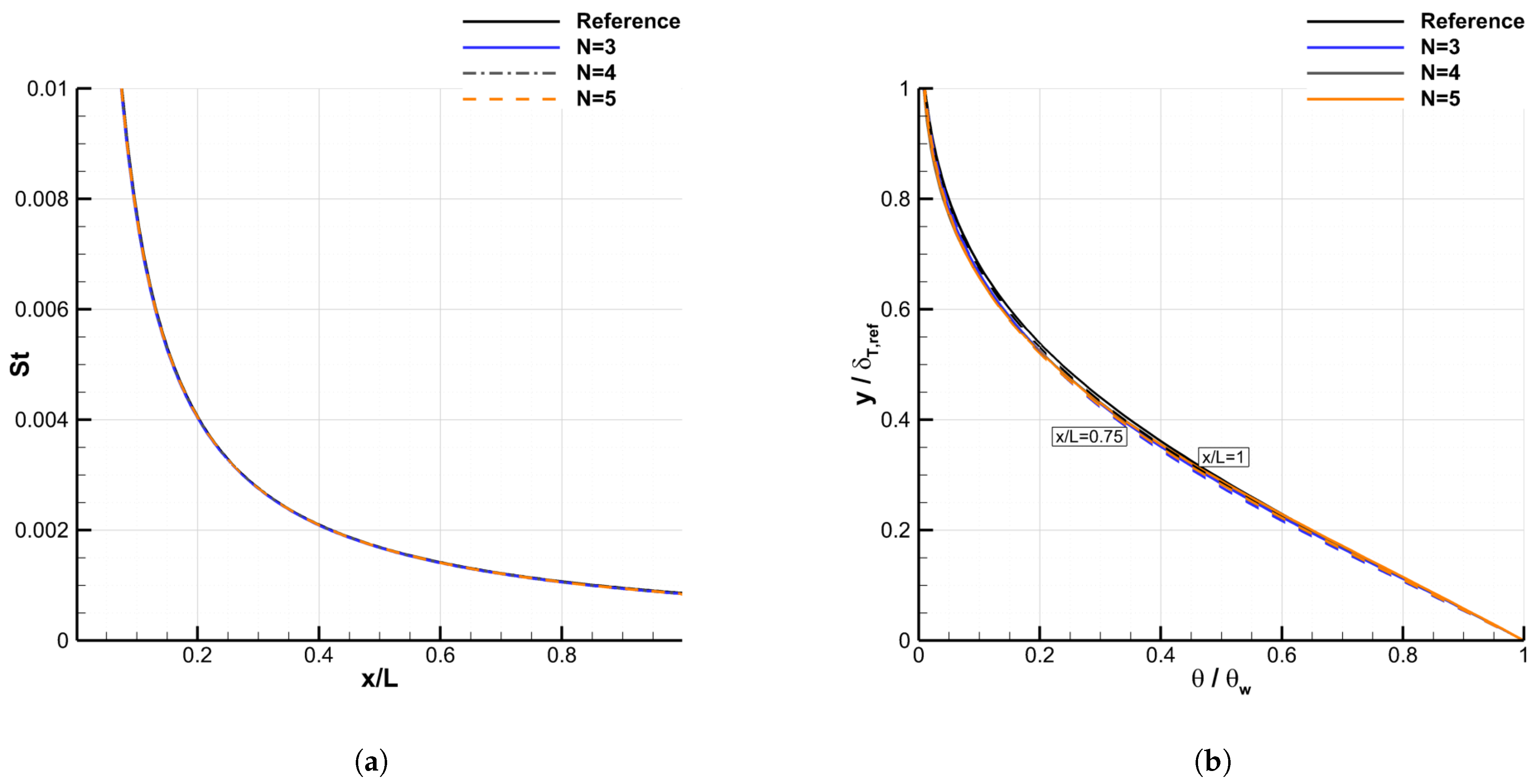
The positive wall temperature gradient test case is such that the wall temperature is 273.15 K for x / L = 0 and 373.15 K for x / L = 1. The wall thus keeps heating the airflow for increasing values of x / L . Figure 16 shows that this situation is less challenging for the modeling than negative wall temperature gradients. Despite the high level of wall temperature gradient addressed, the conclusions are quite similar to the zero-temperature gradient configuration. The solution is converged for N = 4 . As shown in Figure 16a, the wall heat flux is accurately predicted (the relative error is actually lower than 2%). The temperature profiles are almost self-similar and they are accurately predicted by the Galerkin approach.

4.4.4. Uniform Temperature, m = −0.01961

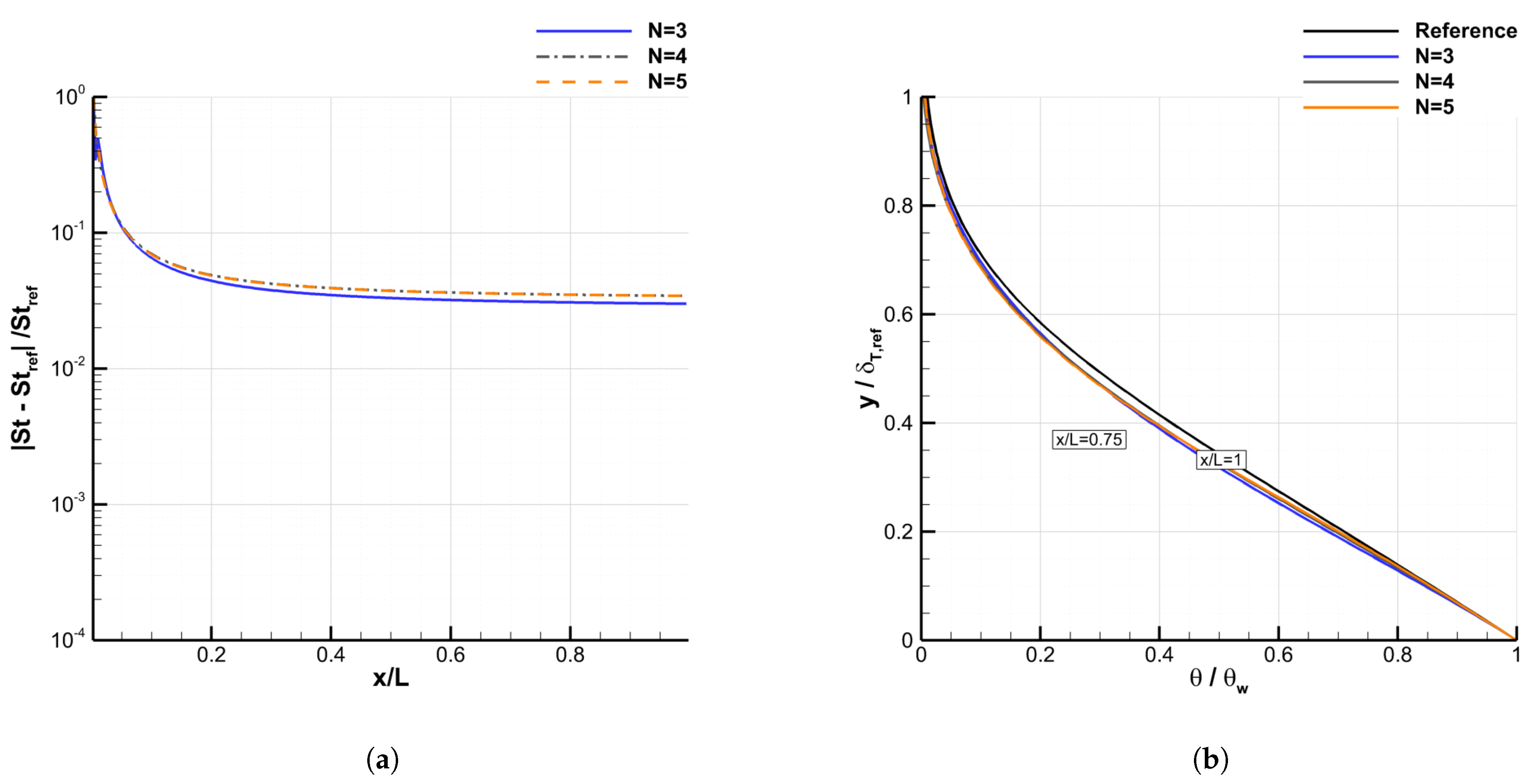
Regarding the decelerated flow with zero wall temperature gradient, the conclusions are not very different from those obtained for m = 1 , except that the error is overall larger. As shown in Figure 17, convergence is achieved for N = 4 . The relative error in the Stanton number is large in the vicinity of x / L = 0 and approaches 4% for x / L = 1 (Figure 17a). As for m = 1 , the slope of the error in S t versus x / L is consistent with the slope observed for the error in the velocity (which also decreases with x). This confirms the major effect of the velocity profile provided as input to the calculation. Moreover, the catastrophic level of error for low x / L is actually deemed to be less representative of the behavior of the method than the final 4% error. A growing error in the dynamic boundary-layer resolution was indeed also observed in the vicinity of x / L = 0 for decelerated wedge flows in the paper of Bayeux et al. [12], but there was not such a strong error in the decelerated areas on real airfoils. Regarding the temperature profiles, self-similarity is almost retrieved and all values of N produce similar levels of error, which are higher than for m = 1 (Figure 17b).
As for m = 1 , it has to be noticed that these conclusions remain valid for a heated wall with positive wall temperature gradient (test-case 5).

4.4.5. Uniform Temperature Gradient −400 K/m, m = −0.01961

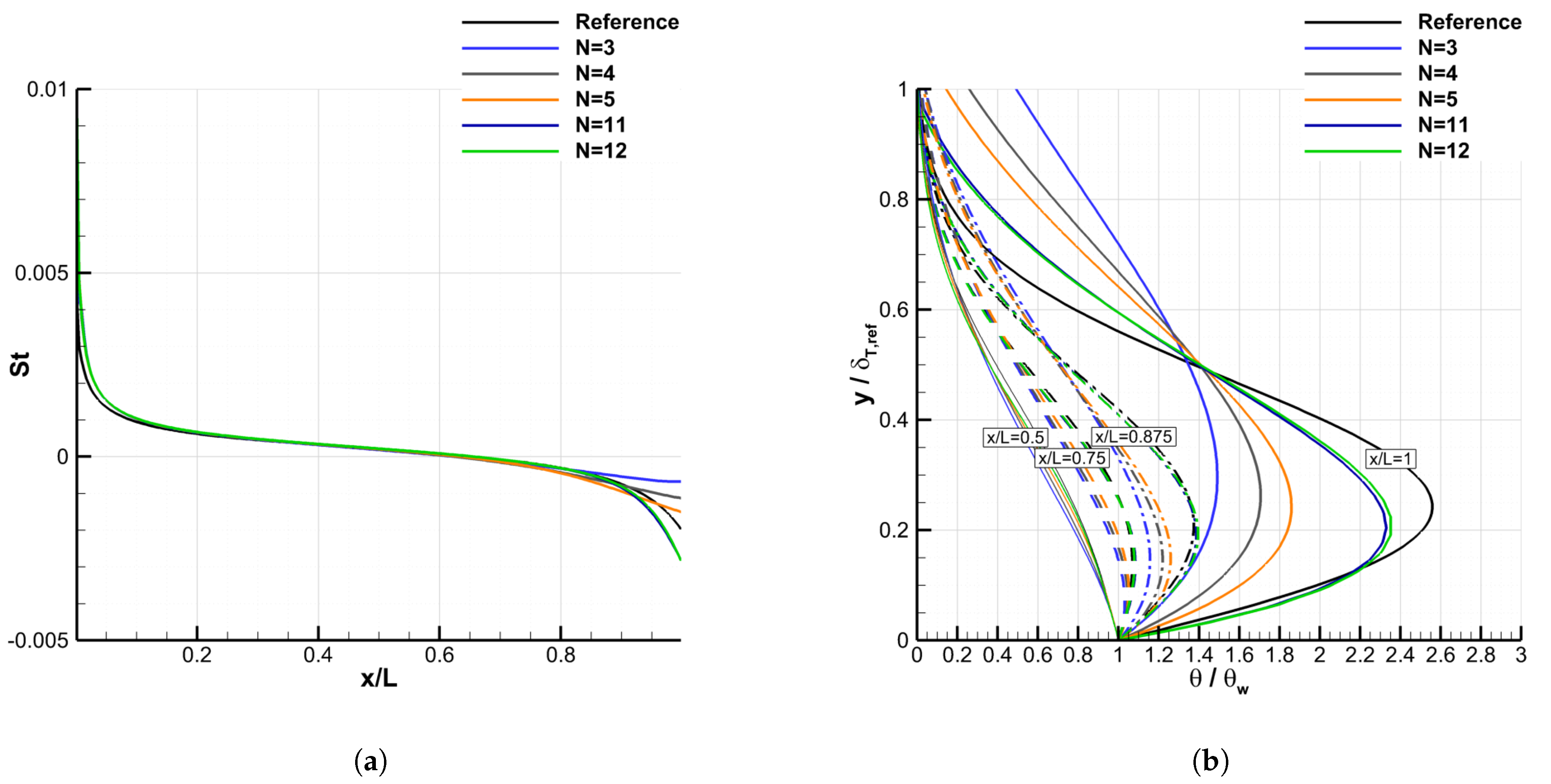
Finally, the decelerated flow with negative wall temperature gradient is even more challenging for the model than for m = 1 . The same conclusions can be drawn, but with higher levels of error, as shown in Figure 18. The number of modes required for achieving convergence is also larger ( N = 12 ). The temperature profile is highly disturbed by the advection of heat from upstream to downstream (Figure 18b). Increasing the number of modes N allows us to better capture the temperature profiles, especially in the vicinity of the wall. As for m = 1 , although the N = 5 solution is not fully converged and does not predict the reference temperature profile very accurately, the prediction of wall heat flux is already quite satisfactory, as shown in Figure 18a.

4.5. Discussion about the Computational Time

It should be noted that the performance of the proposed method in terms of computational time has not been studied in this work. In particular, no effort has been made to optimize the code used. However, we can mention that the simulations performed with N = 4 to 5 modes, which are generally of sufficient accuracy, require only a few tens of seconds of computation on a simple single-core computer.
On the other hand, the computational time increases very quickly with the number N of modes because of the very restrictive stability condition (in O ( 1 / N 2 ) ) on the time step. The future use of a totally implicit time integration method, allowing us to get rid of the stability condition, should allow a gain of several orders of magnitude on the number of time steps necessary to reach the stationary solution and thus significantly increase the performance of the method. Moreover, it should be kept in mind that for applications to aircraft in-flight icing, an important part of the expected time saving comes from the fact that the method should make it possible to replace iterative Navier–Stokes calculations by a viscous inviscid interaction approach, which is much less costly because it requires much less dense meshes near the walls.

5. Conclusions

In this paper, an original numerical method has been presented to solve laminar thermal boundary layers with non-uniform wall boundary conditions. This new method is based on the coupling between a modal method (Galerkin method) in the normal direction to the wall and a finite volume method in the tangential directions, which allows us to use only a surface mesh like an integral method.
Many numerical tests were performed to evaluate its accuracy, to determine the number of modes needed, and to ensure that the method is able to correctly compute the wall heat flux even in the presence of very large wall temperature variations. A series of academic test cases was used, corresponding to wedge flows, representative of the different possible situations encountered on a real airfoil protected by a thermal anti-icing or de-icing system: stagnation point flow, accelerated flow, and decelerated flow, with a positive or negative wall temperature gradient. The solutions obtained with the new method have been compared to those obtained with a finite volume method applied directly to the Prandtl equations of the boundary layer (ONERA’s CLICET code). With only 5 modes, it has been shown that in all cases the relative error on the wall heat flux did not exceed a few percent, which is quite sufficient for the targeted applications considering the numerous other sources of uncertainty. It has also been shown that the origin of this error comes for a large part from the error committed on the prediction of the velocity field used for the resolution of the thermal boundary layer.
Future work will focus on the extension of the method to the case of turbulent boundary layers and on the implementation of the method in the ONERA 3D icing computational suite [26,27]. In particular the possibility of a two-way coupling with the resolution of the dynamic boundary layer will be considered and the explicit time integration scheme used in the present work will be replaced by an implicit scheme to avoid the restrictive stability condition and save computational time. Considering the good results obtained on the 2D laminar cases presented in this paper, this new method is a promising option to build a fast and robust computational suite to simulate the ice accretion on 3D surfaces protected by a thermal anti-icing or de-icing system.

Author Contributions

Conceptualization, P.V., R.H. and E.R.; methodology, P.V., R.H. and E.R.; software, R.H., P.V. and E.R.; validation, E.R.; formal analysis, E.R., P.V. and R.H.; investigation, E.R., P.V. and R.H.; data curation, E.R.; writing—original draft preparation, E.R. and R.H.; writing—review and editing, E.R. and P.V.; visualization, E.R.; supervision, P.V. and E.R.; project administration, E.R. and P.V.; funding acquisition, E.R. and P.V. All authors have read and agreed to the published version of the manuscript.

Funding

This research received no external funding.

Institutional Review Board Statement

Not applicable.

Informed Consent Statement

Not applicable.

Data Availability Statement

Not applicable.

Acknowledgments

The authors would like to thank G. Blanchard for the supportive and fruitful discussions.

Conflicts of Interest

The authors declare no conflict of interest.

Appendix A. Short Description of the Resolution of the Dynamic Boundary Layer in the Solver BLIM2D

In BLIM2D, the dynamic boundary layer is solved via a two-equation integral boundary-layer model:
t U + x F ( x , U ) = S ( x , U )
where
U = u x e δ 1 u x e 2 δ 2 F = u x e 2 δ 2 u x e 3 δ 3 u x e 3 δ 2 S = u x e δ 1 x u x e + 1 2 u x e 2 C f ( u x e 2 δ 1 u x e 2 δ 2 ) x u x e 1 2 u x e 3 C f + 2 u x e 3 C D
δ 1 , δ 2 and δ 3 correspond to the displacement, momentum and kinetic-energy thicknesses, respectively.
δ 1 = 0 1 u x u x e d y δ 2 = 0 u x u x e 1 u x u x e d y δ 3 = 0 u x u x e 1 u x 2 u x e 2 d y
C f and C D denote, respectively, the friction coefficient and the dissipation coefficient:
1 2 u e 2 C f = τ w ρ , u e 3 C D = 1 ρ 0 τ x y y u d y
τ w is the skin friction. In Equation (A1), the first equation is an unsteady version of the well-known von Kármán equation. The second one is the kinetic energy integral equation. In laminar regimes, this system is closed through the use of the following assumed velocity profile:
u x u x e = 1 1 + a ( H ) η 1 η p ( H ) 1
where η = y / δ , δ is the dynamic boundary-layer thickness, and the parameters a and p are dependent on the shape factor H = δ 1 δ 2 .
The conservative formulation allows the use of a finite volume resolution. A first-order upwind scheme is used and the steady-state solution is reached with a semi-implicit scheme, for which only the source terms are implicit, and with local time-stepping. The interested reader will find further information in Bayeux’s article [12].

Appendix B. Validation of the Model against an Empiric Relation
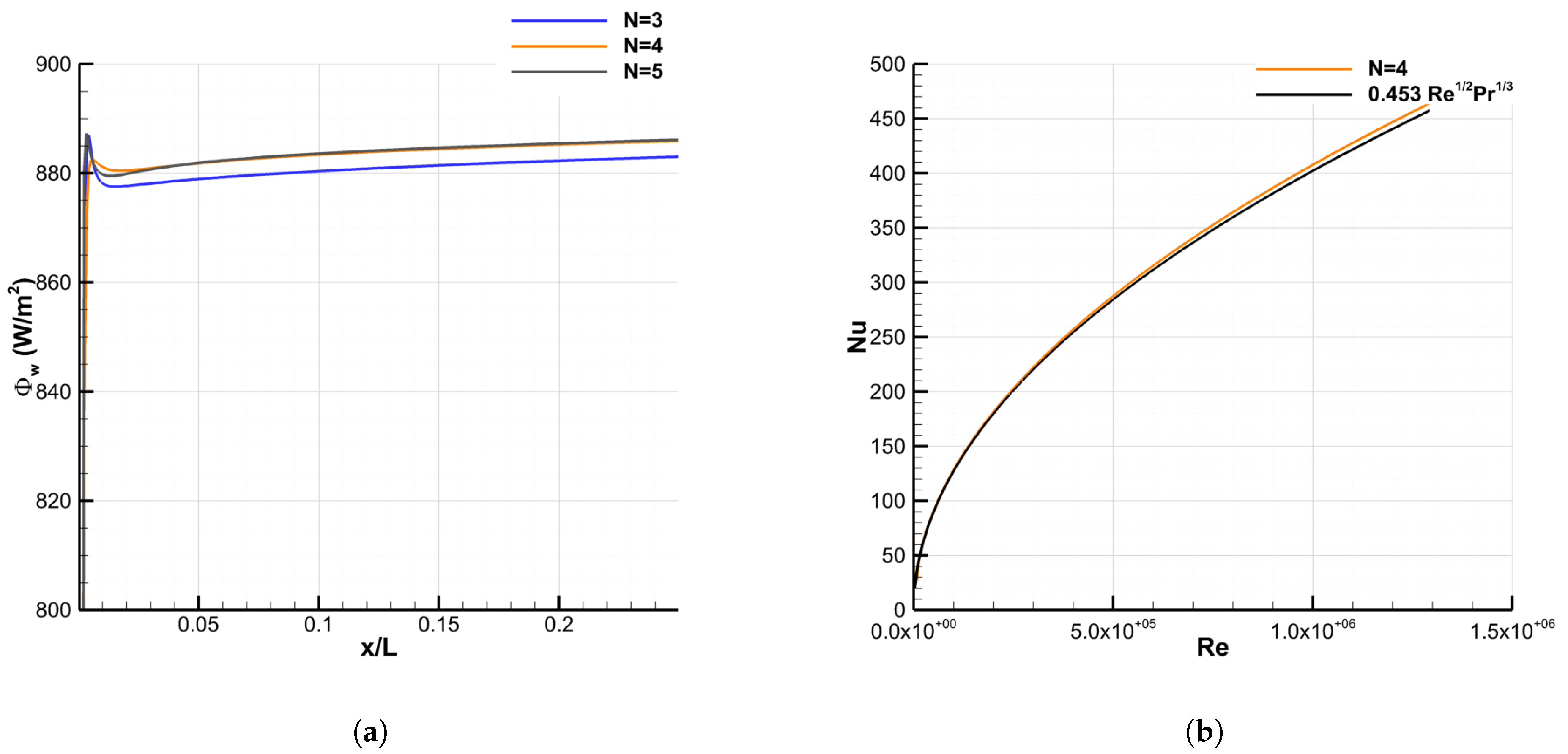
The method was assessed against the empiric relation N u = 0.453 R e 1 / 2 P r 1 / 3 valid for constant heat flux on a flat plate. The Reynolds number is R e = ρ e x u x e μ e , whereas the Nusselt number is N u = h x k , where the heat transfer coefficient is h = ϕ w T w T r . The classic recovery temperature formula is used T r = T e 1 + P r 1 / 2 γ 1 2 M 2 . As stressed by Lienhard [28] for instance, it is expected that imposing a wall temperature varying as x 1 / 2 will lead to a constant wall heat flux along the flat plate. The conditions 3 of Table 1 were used with m = 0 , except that the wall temperature is given by T w T r = 20 x 1 / 2 . Regarding the mesh size, again, N x = 256 . Figure A1a shows that for a number of modes N = 4 , the solution is well converged. The figure also demonstrates that the heat flux is a rather well-predicted constant (relative error around 0.005 ), except in the immediate vicinity of x = 0 . Figure A1b validates the model in terms of Nusselt number for this case with non-uniform wall temperature.
Figure A1. Validation of (a) the wall heat flux and (b) the Nusselt number. Test case 3, with wall temperature varying as x 1 / 2 , m = 0 . N = 3 to N = 5 , N x = 256 .
Energies 15 03267 g0a1

References

  1. Morency, F.; Tezok, F.; Paraschivoiu, I. Anti-icing system simulation using CANICE. J. Aircr. 1999, 36, 999–1006. [Google Scholar] [CrossRef]
  2. Al-Khalil, K.M.; Horvath, C.; Miller, D.R.; Wright, W. Validation of NASA Thermal Ice Protection Computer Codes Part 3: Validation of ANTICE; Technical Report, NASA TM 2001-210907; Glenn Research Center: Cleveland, OH, USA, 2001.
  3. da Silva, G.A.L.; de Mattos Silvares, O.; de Jesus Zerbini, E.J.G. Numerical Simulation of Airfoil Thermal Anti-Ice Operation. Part 1: Mathematical Modeling. J. Aircr. 2007, 44, 627–633. [Google Scholar] [CrossRef]
  4. Wright, W. User’s Manual for LEWICE Version 3.2; Technical Report, NASA/CR-2008-214255; Glenn Research Center: Cleveland, OH, USA, 2008.
  5. Bu, X.; Lin, G.; Yu, J.; Yang, S.; Song, X. Numerical simulation of an airfoil electrothermal anti-icing system. Proc. Inst. Mech. Eng. Part G J. Aerosp. Eng. 2013, 227, 1608–1622. [Google Scholar] [CrossRef]
  6. Morency, F.; Tezok, F.; Paraschivoiu, I. Heat and Mass Transfer in the Case of Anti-Icing System Simulation. J. Aircr. 2000, 37, 245–252. [Google Scholar] [CrossRef]
  7. Croce, G.; Beaugendre, H.; Habashi, W. CHT3D-FENSAP-ICE conjugate heat transfer computations with droplet impingement and runback effects. In Proceedings of the 40th AIAA Aerospace Sciences Meeting and Exhibit, Reno, NV, USA, 14–17 January 2002. [Google Scholar] [CrossRef]
  8. Bu, X.; Lin, G.; Shen, X.; Hu, Z.; Wen, D. Numerical simulation of aircraft thermal anti-icing system based on a tight-coupling method. Int. J. Heat Mass Transf. 2020, 148, 119061. [Google Scholar] [CrossRef]
  9. Henry, R. Development of an electrothermal de-icing/anti-icing model. In Proceedings of the 30th Aerospace Sciences Meeting and Exhibit, Reno, NV, USA, 6–9 January 1992. [Google Scholar] [CrossRef]
  10. Chauvin, R.; Villedieu, P.; Trontin, P.; Bennani, L. A robust coupling algorithm applied to thermal ice protection system unsteady modeling. In Proceedings of the 6th AIAA Atmospheric and Space Environments Conference, Atlanta, GA, USA, 16–20 June 2014. [Google Scholar] [CrossRef] [Green Version]
  11. Aupoix, B. Couches Limites Bidimensionnelles Compressibles; Descriptif et Mode d’emploi du Code CLICET—Version 2015; Technical Report; ONERA: Toulouse, France, 2015. [Google Scholar]
  12. Bayeux, C.; Radenac, E.; Villedieu, P. Theory and Validation of a 2D Finite-Volume Integral Boundary-Layer Method for Icing Applications. AIAA J. 2019, 57, 1092–1112. [Google Scholar] [CrossRef]
  13. Bayeux, C. Méthode Intégrale pour la Couche Limite Tridimensionnelle. Applications au Givrage. Ph.D. Thesis, Institut Superieur de l’Aeronautique et de l’Espace (ISAE), Toulouse, France, 2017. [Google Scholar]
  14. Radenac, E.; Bayeux, C.; Villedieu, P. Use of a Two-Dimensional Finite Volume Integral Boundary-Layer Method for Ice-Accretion Calculations. AIAA J. 2020, 58, 1592–1606. [Google Scholar] [CrossRef]
  15. Radenac, E.; Kontogiannis, A.; Bayeux, C.; Villedieu, P. An extended rough-wall model for an integral boundary layer model intended for ice accretion calculations. In Proceedings of the 10th AIAA Atmospheric and Space Environments Conference—AVIATION 2018 ATLANTA, Atlanta, GA, USA, 25–29 June 2018. [Google Scholar] [CrossRef]
  16. Harry, R.; Radenac, E.; Blanchard, G.; Villedieu, P. Heat Transfer modeling by integral boundary-layer methods towards icing applications. In Proceedings of the AIAA Aviation 2021 Forum, Virtual, 2–6 August 2021. [Google Scholar] [CrossRef]
  17. Graebel, W.P.; Hsu, C. A Galerkin method for calculation of laminar thermal boundary layers. Int. J. Heat Mass Transf. 1981, 24, 771–774. [Google Scholar] [CrossRef] [Green Version]
  18. Ozdemir, H.; Boogaard, E. Solving the integral boundary layer equations with a discontinuous Galerkin method. In Proceedings of the European Wind Energy Conference and Exhibition 2011, Brussels, Belgium, 13–17 March 2011. [Google Scholar]
  19. Sunden, B.; Wu, Z. On Heat Transfer Issues for Wind Energy Systems. J. Energy Resour. Technol. 2017, 139, 051201. [Google Scholar] [CrossRef]
  20. Lokatt, M.; Eller, D. Finite-volume scheme for the solution of integral boundary layer equations. Comput. Fluids 2016, 132, 62–71. [Google Scholar] [CrossRef]
  21. Prieling, D.; Steiner, H. Analysis of the wall mass transfer on spinning disks using an integral boundary layer method. Chem. Eng. Sci. 2013, 101, 109–119. [Google Scholar] [CrossRef]
  22. Cousteix, J. Aérodynamique et Couche Limite Laminaire; Cepadues Editions: Toulouse, France, 1989. [Google Scholar]
  23. Papadakis, M.; Wong, S.H.; Yeong, H.W.; Wong, S.C. Icing Tunnel Experiments with a Hot Air Anti-Icing System. In Proceedings of the 46th AIAA Aerospace Science Meeting and Exhibit, Reno, NV, USA, 7–10 January 2008. [Google Scholar] [CrossRef]
  24. Aupoix, B. Roughness corrections for the k-ω shear stress transport model: Status and proposals. J. Fluids Eng. 2015, 137, 021202. [Google Scholar] [CrossRef]
  25. Chedevergne, F. Analytical wall function including roughness corrections. Int. J. Heat Fluid Flow 2018, 73, 258–269. [Google Scholar] [CrossRef] [Green Version]
  26. Radenac, E.; Gaible, H.; Bezard, H.; Reulet, P. IGLOO3D Computations of the Ice Accretion on Swept-Wings of the SUNSET2 Database; SAE Technical Paper 2019-01-1935; SAE: Warrendale, PA, USA, 2019. [Google Scholar] [CrossRef]
  27. Bempedelis, N.; Bayeux, C.; Blanchard, G.; Radenac, E.; Villedieu, P. A 3D Finite-Volume Integral Boundary Layer method for icing applications. In Proceedings of the 9th AIAA Atmospheric and Space Environments Conference, Denver, CO, USA, 5–9 June 2017. [Google Scholar] [CrossRef] [Green Version]
  28. Lienhard, J.H. Heat Transfer in Flat-Plate Boundary Layers: A Correlation for Laminar, Transitional, and Turbulent Flow. J. Heat Transf. 2020, 142, 061805. [Google Scholar] [CrossRef] [Green Version]
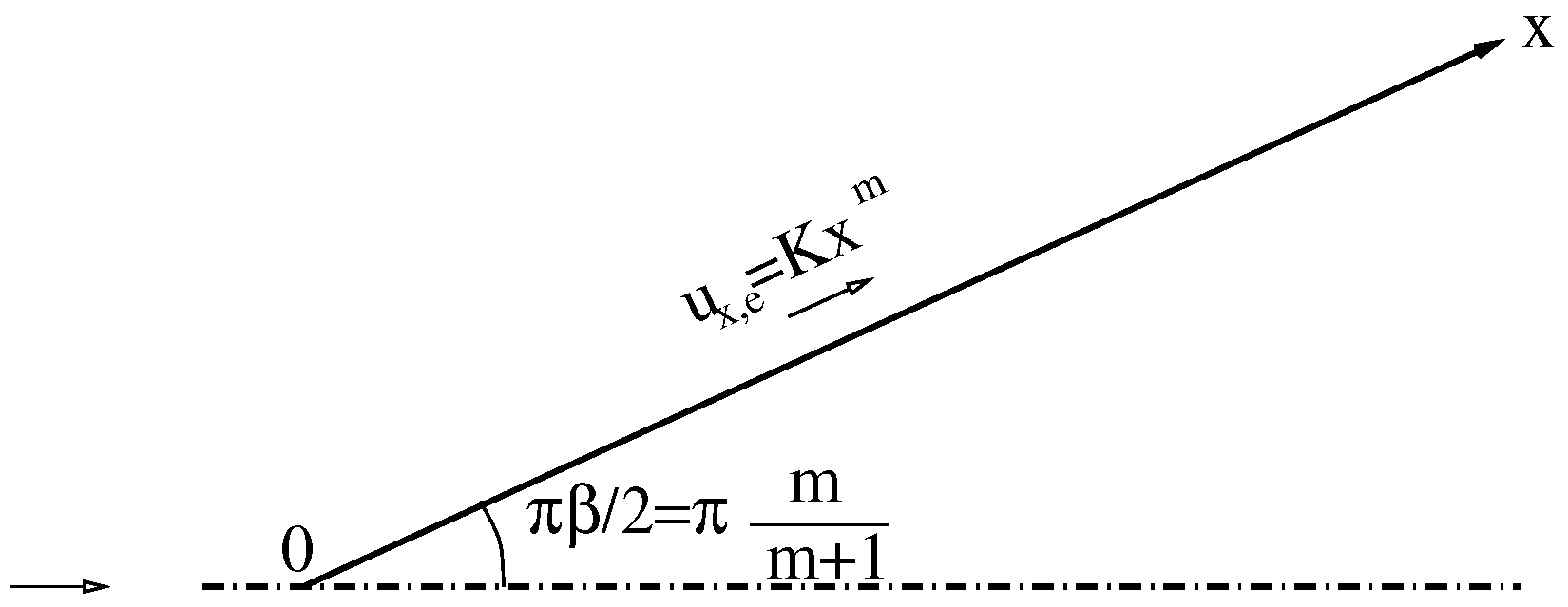
Figure 1. Definition of the wedge-flow geometry.
Energies 15 03267 g001
Figure 2. Velocity profiles for CLICET (reference) and BLIM2D, at x / L = 1 . Test case 1, N x = 256 .
Energies 15 03267 g002
Figure 3. Source terms for N = 5 . (a) Equation (1), (b) Equation (2). Test-case 1, N x = 256 .
Energies 15 03267 g003
Figure 4. Non-dimensional temperature profiles for N = 4 at all the points of the grid. Test case 1, N x = 256 .
Energies 15 03267 g004
Figure 5. ϕ w for N x = 64 to N x = 512 . Test case 1, N = 4 .
Energies 15 03267 g005
Figure 6. Relative error in ϕ w for N x = 64 to N x = 256 . Test case 1, N = 4 .
Energies 15 03267 g006
Figure 7. θ j for N = 1 to N = 5 : (a) θ 1 , (b) θ 2 . Test case 1, N x = 256 .
Energies 15 03267 g007
Figure 8. δ T for N = 1 to N = 5 , and for the reference CLICET solution (solid lines). δ T / ( q + 1 ) for N = 1 to N = 5 (dashed lines). Test case 1, N x = 256 .
Energies 15 03267 g008
Figure 9. Temperature for N = 1 to N = 5 , and for the reference CLICET solution. (a) temperature profiles at x / L = 1 , (b) error. Test case 1, N x = 256 .
Energies 15 03267 g009
Figure 10. Stanton number for N = 1 to N = 5 , and for the reference CLICET solution. (a) Stanton number, (b) relative error. Test case 1, N x = 256 .
Energies 15 03267 g010
Figure 11. Velocity in test-case 2. (a) velocity profiles, m = 1 , x / L = 1 , (b) L2 relative error. Impact of the wall temperature changes on the profiles. The errors of test cases 3, 4 and 5 are super-imposed (large case size: u x ; small case size: u y ). N x = 256 .
Energies 15 03267 g011
Figure 12. L 2 relative error in the wall heat flux in test-case 2 with respect to the wall temperature. The results of test cases 3, 4 and 5 are super-imposed. N x = 256 , N = 4 .
Energies 15 03267 g012
Figure 13. (a) Stanton number for N = 3 to N = 5 and (b) relative error in the Stanton number. Test case 3, m = 1 . N x = 256 .
Energies 15 03267 g013
Figure 14. Temperature profiles for several x / L locations, and for the reference CLICET solution. Test case 3, m = 1 . N x = 256 .
Energies 15 03267 g014
Figure 15. (a) Stanton number and (b) temperature profiles for several x / L locations. Test case 4, m = 1 . N = 3 to N = 10 , N x = 256 .
Energies 15 03267 g015
Figure 16. (a) Stanton number and (b) temperature profiles for several x / L locations. Test case 5, m = 1 . N = 3 to N = 5 , N x = 256 .
Energies 15 03267 g016
Figure 17. (a) Error in the Stanton number and (b) temperature profiles for several x / L locations. Test case 3, m = 0.01961 . N = 3 to N = 5 , N x = 256 .
Energies 15 03267 g017
Figure 18. (a) Stanton number and (b) temperature profiles for several x / L locations. Test case 4, m = 0.01961 . N = 3 to N = 12 , N x = 256 .
Energies 15 03267 g018
Table 1. Physical parameters for the test cases. M is the Mach number at the end of the plate ( x = L ), T w 0 is the wall temperature at x = 0 , p i e and T i e are the total pressure and total temperature of the edge flow, respectively.
Test-CaseL (m)mM p ie (Pa) T ie (K) T w 0 (K) T w · e x (K/m)
10.2510.0180,005263.155264.150
20.25−0.01961, 0, 1/3, 10.0180,005263.155264.15, 273.15, 323.15, 373.150
30.25−0.01961, 0, 1/3, 10.2583,555266.439323.150
40.25−0.01961, 0, 1/3, 10.2583,555266.439373.15−400
50.25−0.01961, 0, 1/3, 10.2583,555266.439273.15400
Publisher’s Note: MDPI stays neutral with regard to jurisdictional claims in published maps and institutional affiliations.