Article

Data-Driven Calibration of Rough Heat Transfer Prediction Using Bayesian Inversion and Genetic Algorithm

1
Mechanical Engineering Department, École de Technologie Supérieure, Montréal, QC H3C1K3, Canada
2
Institut National de Recherche en Informatique et en Automatique (INRIA), F-33405 Talence, France
3
University Bordeaux, INRIA, CNRS, Bordeaux INP, IMB, UMR 5251, F-33400 Talence, France
*
Author to whom correspondence should be addressed.
Energies 2022, 15(10), 3793; https://doi.org/10.3390/en15103793
Submission received: 19 April 2022 / Revised: 18 May 2022 / Accepted: 20 May 2022 / Published: 21 May 2022
(This article belongs to the Special Issue Aerodynamics and Heat Transfer for Aircraft and Aerospace Systems)

Abstract

:
The prediction of heat transfers in Reynolds-Averaged Navier–Stokes (RANS) simulations requires corrections for rough surfaces. The turbulence models are adapted to cope with surface roughness impacting the near-wall behaviour compared to a smooth surface. These adjustments in the models correctly predict the skin friction but create a tendency to overpredict the heat transfers compared to experiments. These overpredictions require the use of an additional thermal correction model to lower the heat transfers. Finding the correct numerical parameters to best fit the experimental results is non-trivial, since roughness patterns are often irregular. The objective of this paper is to develop a methodology to calibrate the roughness parameters for a thermal correction model for a rough curved channel test case. First, the design of the experiments allows the generation of metamodels for the prediction of the heat transfer coefficients. The polynomial chaos expansion approach is used to create the metamodels. The metamodels are then successively used with a Bayesian inversion and a genetic algorithm method to estimate the best set of roughness parameters to fit the available experimental results. Both calibrations are compared to assess their strengths and weaknesses. Starting with unknown roughness parameters, this methodology allows calibrating them and obtaining between 4.7% and 10% of average discrepancy between the calibrated RANS heat transfer prediction and the experimental results. The methodology is promising, showing the ability to finely select the roughness parameters to input in the numerical model to fit the experimental heat transfer, without an a priori knowledge of the actual roughness pattern.

Graphical Abstract

1. Introduction

The numerical simulation of airflow above a rough wall differs from a classical smooth wall situation. The surface roughness creates a different near-wall behaviour, especially for the skin friction and the heat transfers. This led to the modification of the classical turbulence models to account for the roughness elements, like in [1] for the Spalart–Allmaras model. The main characteristics of the rough extension of the Spalart–Allmaras model reside in setting a non-zero turbulence viscosity at the wall. Usually, these adapted models are specifically designed to predict the correct skin friction coefficients based on experimental benchmark cases. This attention given to the skin friction coefficients alone has a drawback: the predicted heat fluxes are higher than the experimentally measured ones. An additional thermal correction model is thus required to adjust heat fluxes. To correct the heat flux behaviour, [2] suggested increasing the turbulent Prandtl number close to the wall. Further thermal correction model developments carried out by [3] and recently by [4] continued to aim at a turbulent Prandtl increase.
The thermal correction models take as input various parameters describing the roughness pattern of the surface. These parameters can be physically measurable, such as the roughness height, or numerical, such as the equivalent roughness. For instance, the thermal correction of [3] takes three input parameters and the two-parameter Prandtl correction (2PP) of [4], takes two. The latter 2PP thermal correction model is the one used in the present study. Previous works highlighted that the heat flux is sensitive to those roughness parameters and to the thermal correction model itself [4,5]. Usually, the equivalent roughness is computed from the roughness shape using empirical relations such as [6]. Those relations were built using manufactured regular roughness patterns, such as regularly spaced cones, hemispheres or pyramids. In many real-life situations, for example in aircraft icing [7], roughness patterns are irregular and present several uncertainties. Therefore, classical empirical relations can fail to correctly describe a roughness pattern in such situations.
To avoid the dependence on empirical relations in rough heat transfer CFD simulations, a data-driven approach can be used, provided that experimental data are available. This data-driven approach allows the recovery of the roughness parameters to input in the numerical model by processing the experimental data, without an a priori knowledge of the real roughness pattern. Machine learning and data-driven techniques have already been successfully applied in CFD, for example for the calibration of the turbulence model’s constants in [8], highlighting its potential.
Usually, the data-driven approach relies on metamodels. One of the most common metamodel families is the polynomial chaos expansion (PCE) [9]. PCE metamodels are commonly used in problems where uncertainty propagation is studied, like in [10] and [11]. Most of the time, the PCE approach allows building efficient metamodels from a CFD database, and these are used in lieu of the time-consuming CFD model [12] for complex analyses. The PCE metamodeling was successfully applied in heat transfer applications, for instance in [13] or [14], highlighting its suitability for the present study. Globally, the coupling between PCE metamodeling and CFD has been extensively developed and applied during the last two decade [15,16]. Once the metamodels are established, the sensitivity analysis can be performed, usually using the Sobol indices [17]. This combination of PCE metamodels with Sobol sensitivity indices was previously used in a related work [5]. The Sobol indices allows the classification of the uncertain inputs according to their influence on the particular output of interest of a study using a variance-based approach. These commonly used indices are regularly employed in CFD sensitivity analysis [18]. Following the definition of the metamodels, the calibration of uncertain roughness parameters can be performed. In the present work, two calibration methods will be assessed and compared: the Bayesian inversion and the genetic algorithm. The Bayesian inversion is a commonly used tool allowing model calibration and fine-tuning of numerical parameters [19]. The Bayesian inversion transforms the initial uncalibrated input’s distribution into a refined posterior distribution, whose peak corresponds to the calibrated value [20]. This approach, using probability distributions instead of fixed values, allows flexibility in the interpretation of the calibration results. This calibration methodology was used in the context of the constant calibration of turbulence models [21]. Fine tuning and optimization tasks suit the application of Bayesian inversion. The authors of [22] used Bayesian inversion for the shape optimization of a wall to obtain a prescribed pressure gradient distribution. This application presents similarities with the present work aiming at optimizing the surface roughness to obtain a given heat flux distribution. On the other side, classical calibration methods (i.e., non-Bayesian), such as the genetic algorithm, usually work in a non-probabilistic way, making their calibrated results strictly defined, without controlled flexibility. Classical calibration methods imply more intervention from the human modeller in post-processing, making the final results sensitive to the modeller’s experience, expertise and biases [23]. A genetic algorithm calibrates the problem using an approach similar to biological evolution [24]. The final calibrated parameters are estimated by performing a method using selections, mutations and crossings between “generations” of parameters samples, like in the natural selection process. This type of calibration with genetic algorithm was already used in CFD applications [25], and more specifically for optimization, like in [26] or [27]. This use of genetic algorithms in the CFD field highlights the suitability of the method for the current application. The coupling between the PCE metamodeling and the optimization by Bayesian inversion or genetic algorithm was already used in numerical heat transfer applications [28], showing the potential of the methodology. Additionally, in case of a low trustworthiness metamodel, coupling it with a Bayesian analysis allows one to consider the metamodel’s uncertainty in the whole study [29].
The objective of this paper is to set up a methodology to calibrate the roughness parameters to input into the 2PP thermal correction model to match the experimental results of a given test case. More specifically, a rough curved channel geometry, inspired by [2], is used to set up the design of experiment (DOE) for heat transfers. Next, the DOE allows the generation of PCE metamodels predicting key features of the heat transfers on the wall. The next step is the sensitivity study, using the Sobol indices to identify the most sensitive parameters. Finally, the PCE metamodels are used in a calibration procedure to establish the roughness input parameters with the aim of retrieving the experimental heat transfer distribution in the curved channel. The calibration is done successively with a Bayesian approach and a genetic algorithm to compare both methods on the results discrepancies and practical application.
First, the test case geometry and setup will be described. Second, the 2PP thermal correction model is detailed, highlighting the role of the roughness parameters in the simulation. Next, the DOE construction is depicted prior to the description of the PCE metamodeling, the sensitivity study and the calibration procedures. Finally, the results are shown and compared, highlighting between 4.7% and 5.4% of average discrepancy after the Bayesian calibration compared to the experimental results. On the other side, the genetic algorithm approach gives between 5.7% and 10% of discrepancies.

2. Test Case Geometry and Setup

A specific curved channel test case is used for the application of the depicted methodology. This section will give details about the geometry used in the present study, along with the RANS setup to perform the flow simulation. The geometry and computational domain is detailed, prior to the domain mesh and numerical RANS configuration.

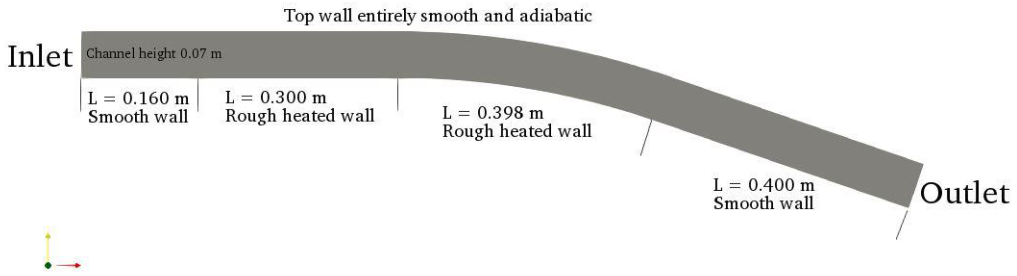
2.1. Physical Geometry and Boundary Conditions

The geometry used to apply the calibration work discussed in this paper is a curved channel experimentally studied by [30]. This test case was numerically studied by [2] few years later. The channel has a straight section followed by a curved one and another straight section. The channel height is 0.07 m while the overall curvilinear length is about 1.25 m. More specifically, the zone of interest is the rough bottom floor of the channel where the heat transfer coefficient will be monitored. Figure 1 illustrates the computational domain.
The curved part of the channel’s floor, whose curvilinear length is 0.398 m, is an arc of radius 1.200 m and an angle of 19°. The freestream values are a velocity magnitude of 40 m/s, an inlet total pressure of 102,304 Pa and a total temperature of 288.95 K. The boundary conditions are also displayed on Figure 1. The floor is divided into three main zones: an initial smooth and unheated wall, the rough and heated study zone (including the curved portion), and a downstream smooth unheated zone. The top wall is entirely smooth and adiabatic. The heated zones are isothermal at 303.15 K and their roughness parameters are the objective of the calibration. The roughness parameters’ distribution will be detailed in Section 4.

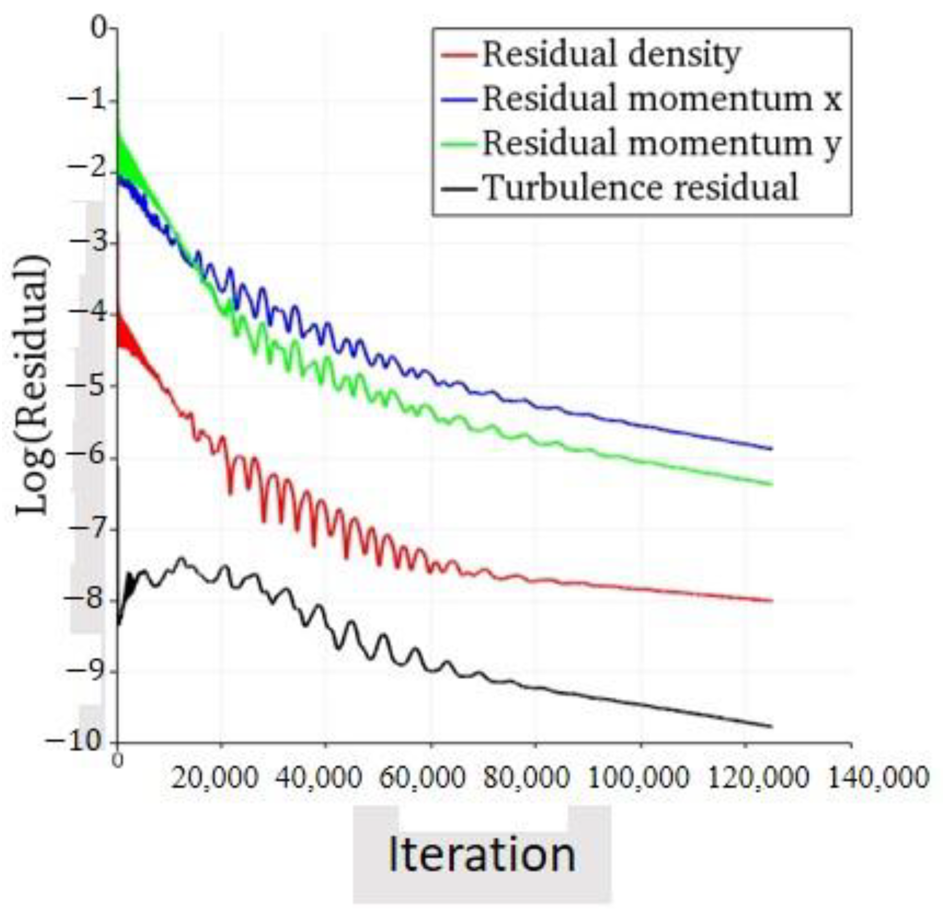
2.2. Mesh and Numerical Setup

The geometry is discretized using quadrilateral elements in a structured mesh. The rough zone of interest is composed of 499 nodes in the stream-wise direction, while the channel height has 399 elements. Coarser meshes were tested, giving similar results on the benchmark test cases. The finest mesh was retained to cope with the various untested roughness patterns planned to be run during the sampling of the DOE. The entire computational grid has 274,512 quadrilaterals. The first cell height is about 3 µm, which allows a y+ below 1 for all the roughness ranges tested. The growth rate normal to the wall is 1.1. A close-up on the mesh near the floor is shown on Figure 2. The main outcomes of the mesh convergence study are detailed in the Appendix A.
The flow simulation is performed using the compressible RANS solver SU2 6.2 [31]. The Reynolds number based on the total floor length is 3.2 × 10 6 and the Mach number is 0.118. To accelerate the convergence, the CFL number is set to 10. Finally, the convective fluxes are discretized using a Roe scheme with MUSCL reconstruction [32]. The solver used includes in-house implementations of the rough modification of the Spalart–Allmaras turbulence model [1] and the addition of the 2PP [4] thermal correction model. The next section will detail the mathematical model making up the thermal correction model.

3. 2PP Thermal Correction Model

This section will give an overview of the equations of the 2PP thermal correction model. The 2PP thermal correction model was implemented into SU2, and aims at increasing the Prandtl number in the near-wall region to reduce the heat flux when the rough version of the Spalart–Allmaras turbulence model is used.
The 2PP thermal correction model achieves the goal of increasing the turbulent Prandtl number by computing an increment ΔPrt. The model takes two roughness input parameters: the roughness height k (m) and the equivalent roughness ks (m). Equation (1) allows the computation of ΔPrt. In Equation (1), Pr is the laminar Prandtl number and d is the distance to the wall.
Δ P r t = g × 0.07083 × R e s 0.45 × P r 0.8 × e x p d k
The roughness Reynolds number and the parameter g in Equation (1) are detailed in Equations (2) and (3).
R e S = u τ k s ν
g = 1     if   R e s 70 g = ln R e s ln 5 ln 70 ln 5   if   5 < R e s < 70 g = 0     if   R e s 5
In Equation (2), u τ is the friction velocity, and ν is the air kinematic viscosity. Finally, Equations (1)–(3) highlighted that the roughness parameters have a direct impact on the Prandtl number correction, and thus on the predicted heat flux.

4. PCE Metamodeling

This section will depict the metamodeling process retained, using polynomial chaos expansion (PCE) metamodels. This step allows the creation of metamodels to predict the heat flux behaviour above any roughness pattern without the need for a complete CFD run. The first step of the metamodeling task is the creation of a numerical DOE. The PCE metamodels are then generated, and finally their accuracy is checked to ensure they are reliable enough for the study.

4.1. Design of Experiment (DOE)

To prepare the metamodeling and calibration steps, a numerical DOE of heat transfers for various roughness patterns is needed. First, the distribution of the input parameters k and ks/k are defined to set the ranges for the sampling. Note that the ratio ks/k is used instead of ks alone, since it will allow one to directly evaluate the relation between the roughness height and the equivalent roughness. The present work is included in the broader scope of in-flight aircraft icing. Therefore, the typical ranges of variation of k and ks/k are obtained from the icing literature [33,34]. These ranges are wide enough to ensure that they are suitable for the current study, which is not specifically a simulation in icing conditions. The compilation of the distribution of all the input parameters is given in Table 1. The distributions are chosen as uniform since there is no a priori knowledge of the experimental roughness pattern.
Following the distributions of Table 1, a sampling is done using the Latin hypercube sampling [35]. The sample size is defined according to the literature [36] for a response surface and gives, with an oversampling factor, 120 samples. Following the sampling, 120 CFD simulations of the curved channel are run. This allows the construction of a numerical heat transfer database, needed for the next metamodeling step.

4.2. Metamodels Generation

Once the heat transfer DOE is set up and ran, the metamodeling tool uses its output database to estimate a mathematical relation between the roughness parameter inputs and the heat flux output. For this study, polynomial chaos expansion (PCE) metamodels were chosen [9] and generated using the UQLab tool [9]. The choice of this type of metamodel is motivated by its wide use in uncertainty quantification for CFD and aerodynamic applications [37]. The general form of a PCE metamodel is given by Equation (4).
Y i = M i X = α y α × ψ α X
In Equation (4), Yi is the output of interest, X = (X1, X2) is the input parameter vector, Mi is the corresponding PCE metamodel defined by its coefficients y α and the multivariate polynomials ψ α of the decomposition. α = (α1, α2) is the multi-index with two components (since there are two input parameters; see Table 1). The multivariate polynomials ψ α are obtained as the tensor product of the two (in the present application) univariate basis polynomials φ (Equation (5)).
ψ α X = i = 1 2 φ α i ( X i )
The input parameters having a uniform distribution, the univariate basis polynomials are Legendre polynomials of indices αi [9].
Three metamodels are generated, as listed in Table 2 where hc is the heat transfer coefficient in W/m2K.
The second metamodel, M2, predicts the mean relative error compared to the experimental results of [2]. The mean relative error ε is the average of the relative errors taken on every mesh point (Equation (6)).
ε = 1 N p o i n t s i = 1 N p o i n t s h c , C F D i h c ,   E X P i h c ,   E X P i
In Equation (6), Npoints is the number of mesh points in the study zone, and hc,CFDi and hc,EXPi are the CFD predicted hc at point i and the experimental hc at point i, respectively.
M3 is a multi-output metamodel evaluating in one estimation N values of hc along the wall. Setting N to a high value allows one to predict the complete hc distribution on the entire rough wall. The metamodel M1 is separated from the metamodel M3: this separation allows one to compare the cases where the starting hc is calibrated alone (M1) and where several locations are simultaneously calibrated (M3).
Once a metamodel is created, its evaluation on the inputs of the DOE allows the comparison of its prediction with the actual CFD prediction obtained when setting up the DOE. Doing a linear regression between the PCE prediction and the CFD output allows the computation of the R2 coefficient (Equation (7)).
R 2 = 1 Y C F D Y P C E 2 ( Y C F D Y ¯ C F D ) 2
In Equation (7), YCFD and YPCE are the CFD and PCE predictions, respectively. Y ¯ C F D is the mean value of the output of interest (CFD). An R2 coefficient close to 1 ensures a PCE metamodel with a good accuracy, since it predicts outputs close to what the full CFD simulation gives. Once the metamodels are established, the next step is to use them for the sensitivity study and the calibration purpose.

5. Sensitivity Study

The sensitivity study allows the identification of the most sensitive parameter(s) in the model. Using the previously described PCE metamodels, the sensitivity analysis computes the Sobol indices, described in [17]. These indices allow the classification of the input parameters from the most to the least sensitive. The Sobol index is a ratio of variances, taking values between 0 and 1. For input parameters i and j, the first and second order Sobol indices are defined by Equations (8) and (9), respectively.
S i = V Y E V Y | X i V Y
S i , j = V Y E V Y | X i ,   X j   V Y
In Equations (8) and (9), Y is the output of interest, V is the variance operator, E the mean value, and the notation Y|Xi denotes the output of interest when the ith input parameter is fixed. The total Sobol index, which is monitored in the present study, for the ith input parameter for a generic three parameters study is given by Equation (10).
S T i = 1 S j + S k + S j , k
The total Sobol index gives the contribution of the variability of the ith input and its interactions with the other inputs (here the jth and kth) on the response sensitivity. A total Sobol index close to zero means that the ith parameter does not contribute much to the variability of the studied output. According to the classification criteria suggested by [38], an input parameter with a total Sobol index:
  • above 80% is very important;
  • between 50% and 80% is important;
  • between 30% and 50% is unimportant;
  • below 30% is negligible.

6. Model Calibration

Observing experimental results without an a priori knowledge of the roughness pattern is not helpful to precisely extract the roughness parameters. This task is even more non-trivial since the roughness parameters to input in the model vary depending on the thermal correction model chosen. The calibration is intended to estimate those roughness parameters by working on the PCE metamodels previously created. The Bayesian inversion calibration is first described prior to the genetic algorithm approach.

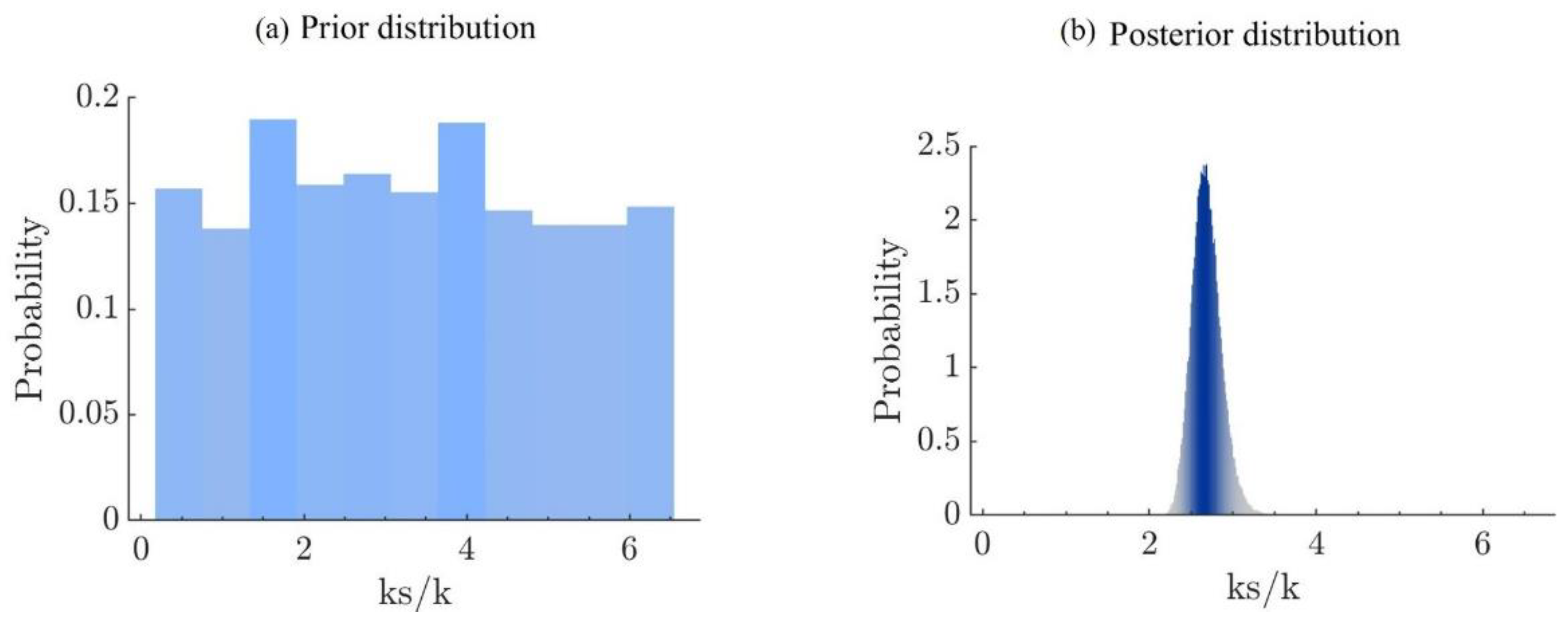
6.1. Bayesian Inversion Calibration

Based on the Bayes theorem (Equation (11)), the principle of the Bayesian inversion is to get the posterior distributions π(θ|Xi) of input Xi, based on the assumed prior distributions (see Table 1) π(θ) and on the information provided by the experimental data. Here, θ denotes the distribution parameters and the | symbol denotes the conditional dependence. The posterior distributions are the distributions of the input parameters knowing the information brought by the experimental data.
π θ | X i = π X i | θ · π θ π X i
In Equation (11), π(Xi|θ) is called the likelihood function and π(Xi) is seen as a normalization constant called the marginal likelihood. The new posterior distributions are generally not uniform anymore and allow identifying the input parameter values that will produce an output that best fits the experimental data. Additionally, a discrepancy between the PCE output and the CFD prediction is given to the solver, along with the experimental observations themselves. For instance, a discrepancy between 0 W/m2K and 15 W/m2K means that up to 15 W/m2K of difference between the PCE and CFD predictions is expected. Numerically speaking, the Bayesian inversion is performed with the UQLab tool [19]. The computation of the posterior distribution is made using a Markov chain Monte Carlo (MCMC) algorithm. The samplers used in the study are the affine invariant ensemble algorithm (AIES) or the Metropolis–Hastings (MH) algorithm. For the purposes of the work, the MCMC solver is tuned to perform 70,000 iterations and generates 15 chains. The Bayesian solver setup for each metamodel is summarized in Table 3. For the metamodel M2 (predicting the mean relative error with experimental data), the experimental observation is 0% of mean relative error. This means that the objective of the calibration is to obtain a mean relative error close to 0%.
After having obtained the posterior distributions, the mean value or the maximum a posteriori (MAP) of these distributions can be estimated. These two statistics can be used to estimate which single values of input parameters lead to a model response close to the experimental data. After evaluating the PCE metamodels and the complete CFD simulation with the calibrated parameters, it is possible to assess the success—or not—of the calibration procedure. One can estimate if the model response is close to the experimental data. Additionally, the distributions of the model predictions using the posterior distributions should present less uncertainty (reduced variance) when using the prior distributions.

6.2. Calibration Using a Genetic Algorithm

The Matlab framework has a built-in genetic algorithm that is used in the study [39,40]. Its purpose is to find the set of input parameters that minimize an objective function. The default settings provided in the Matlab framework provide a straightforward application for the present case. The objective functions supplied to the genetic algorithm are summed up in Table 4.
Note that since the metamodel M3 outputs multiple (N) values, the genetic algorithm is executed N times. Each one of the executions gives a set of calibrated parameters and the final retained parameters are obtained by doing an average or a weighted average over the N solutions. Most of the time, the simple averaging produces unsatisfactory results. The weighted average, with appropriate weight(s) on the most relevant output(s), allows one to improve the results, as shown in the next section.

7. Results

This section will display the results obtained all through the process described in the previous sections. First, the CFD results obtained initially before calibration are shown to illustrate the baseline results. Following this, the characteristics and precision of the metamodels are shown prior to the sensitivity indices. Finally, the calibration results for both Bayesian inversion and genetic algorithm are displayed, prior to the comparison of both methods.

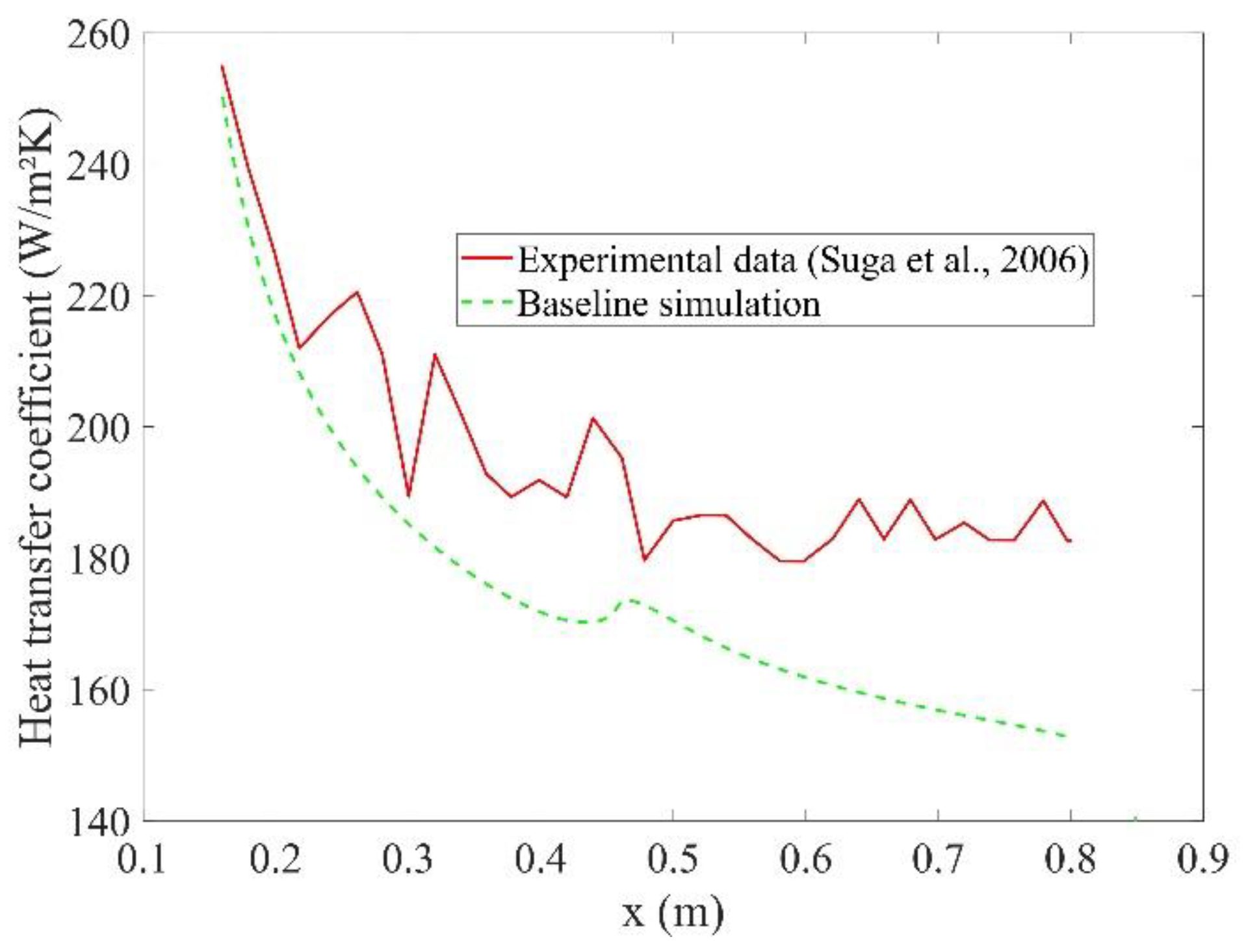
7.1. CFD Results before Calibration

Prior to the metamodeling and calibration process, the curved channel test case, as described in Section 2.1 and Section 2.2, is run alone to verify the CFD settings and mesh. This initial simulation, called here the baseline simulation, is the same as the one run for the mesh study with the fine mesh. The roughness height is k = 0.5 mm and the equivalent roughness is ks = 1.55 mm. This baseline simulation also provides useful information about the convergence of the CFD configuration used. The iterative convergence residual curves are displayed on Figure 3.
Figure 3 shows that after the prescribed number of iterations (125,000), the residuals are stable and decreased by at least three orders of magnitude. The configuration used has a satisfactory convergence behaviour which confirms the choice of the numerical setup. The heat transfer results obtained with these settings are plotted on Figure 4.
From Figure 4, it is possible to notice a relatively poor agreement with the experimental data. Finding the best roughness parameters is non-trivial, and it legitimates the use of the data-driven calibration approach used to match the literature.

7.2. Visualization of the DOE outputs

After a sampling of the roughness parameters with the Latin hypercube method, 120 CFD simulations were run. The heat transfer databases obtained from the DOE are plotted in Figure 5, where each one of the black curves is the heat transfer coefficient of one simulation of the DOE. On Figure 5, the experimental data, in red, from the literature are shown.
By observing the experimental results, it is possible to notice oscillations resulting from the experimental uncertainty. Additionally, all the numerical simulations exhibit a sudden bump at x = 0.46 m, where the curved part of the channel starts. This local increase in the heat transfer coefficient is due to the flow acceleration in the curve portion. Studies in [30] quantified this increase in the heat transfer coefficient value at the start of the curve zone to be about 3%. Figure 5 shows that the target experimental results are included in the envelope defined by the sampling CFD simulations. This observation shows that the initial range of roughness parameters chosen contains the a priori unknown experimental values.

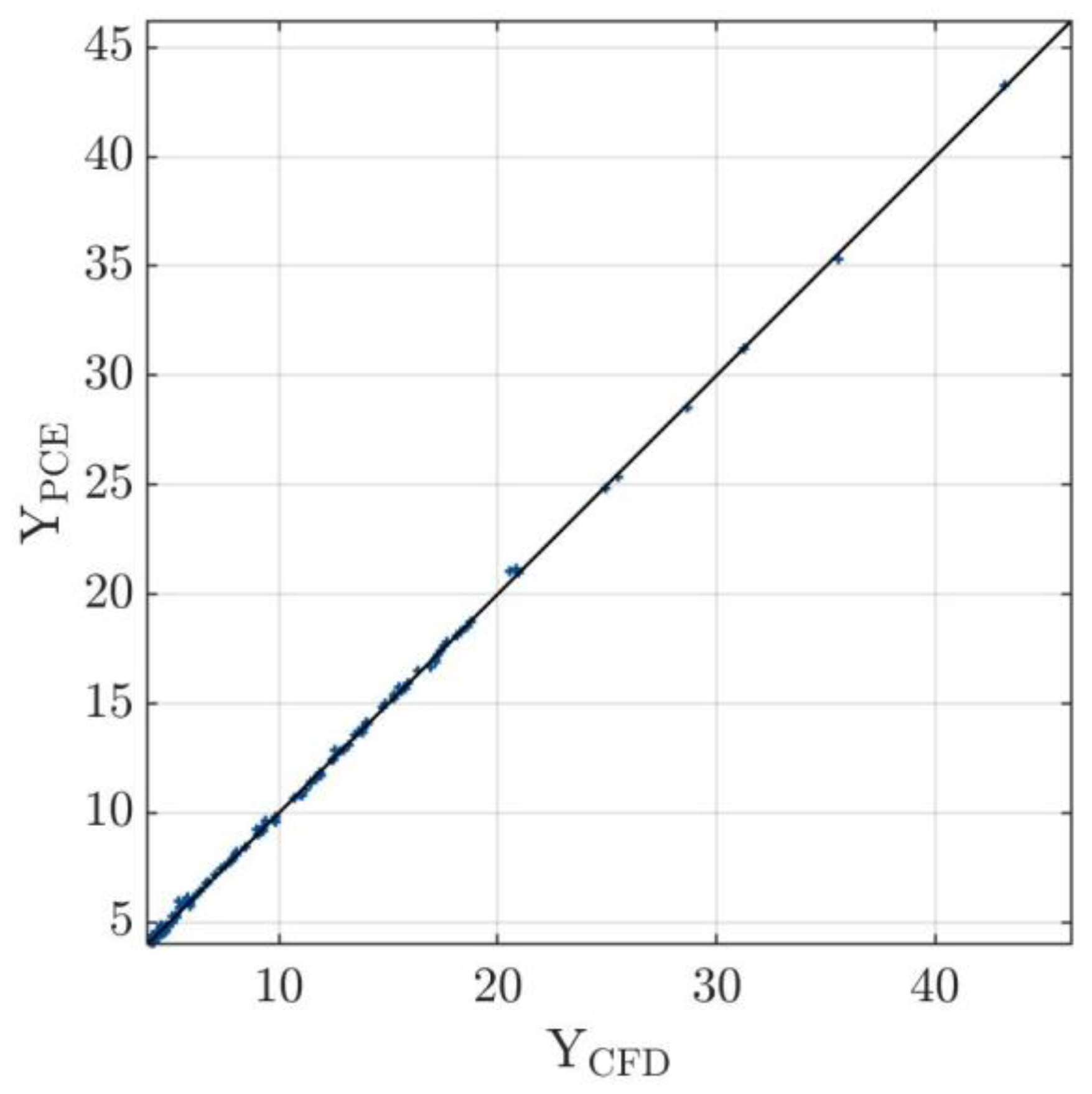
7.3. Characteristics of the Metamodels and Accuracy

The previous DOE is used as a basis for the PCE metamodel generation. Three metamodels are generated: one to predict the initial value of hc along the rough zone, one to predict the mean relative error with experimental results and a third one to predict N values of hc along the wall (see Table 2). For each metamodel, the resulting PCE is described with the polynomial degree pPCE and the number of terms in the expression (Equation (4)). Additionally, the R2 coefficient is calculated to assess the metamodel accuracy (Equation (5)). The values obtained are gathered in Table 5. For the present study and for the rest of the paper, the metamodel M3 is used with N = 6, meaning it computes six values of hc regularly spaced along the wall. Note that the number of terms in Equation (4), for a two input parameters study, is equal to ( p P C E + 2 ) ! p P C E ! 2 ! .
Table 5 shows that the PCEs obtained have a degree between 9 and 12, with the corresponding polynomial expressions having between 55 and 91 terms. All regression coefficients are above 99.9%, meaning an excellent agreement between the CFD results and the PCE-predicted results on the same sample. For comparison, [41] performed the same type of uncertainty quantification analysis with R2 coefficients as low as 94.6%. For graphical visualization, the regression for M2 (with R2 of 99.96%) is plotted on Figure 6 where YPCE and YCFD are the mean errors in percentage with the literature, as predicted by PCE and CFD, respectively. For synthesis and concision, only the regression for M2 is displayed, since it is the worst among the three (see Table 5).
Figure 6 shows that the results are close to the identity line, visually confirming the good value of the R2 regression coefficient. This R2 assessment shows that the metamodels generated are accurate and reliable enough to be used in the present application.

7.4. Sensitivity Study

Using the PCE metamodels, the sensitivity study allows the Sobol indices to be computed (see Equation (8)). Table 6 gathers the total Sobol index values for each metamodel.
Table 6 shows that the roughness height k is the least sensitive parameter in each case, with a total index between 11% and 30%. The ratio ks/k is the most dominant parameter of influence, with 88% to 97% sensitivity. According to the classification made by [38], k is a negligible parameter in the model sensitivity while ks/k is a very important parameter. Therefore, the relation between ks and k is more critical for the model output than their absolute values in millimetres.

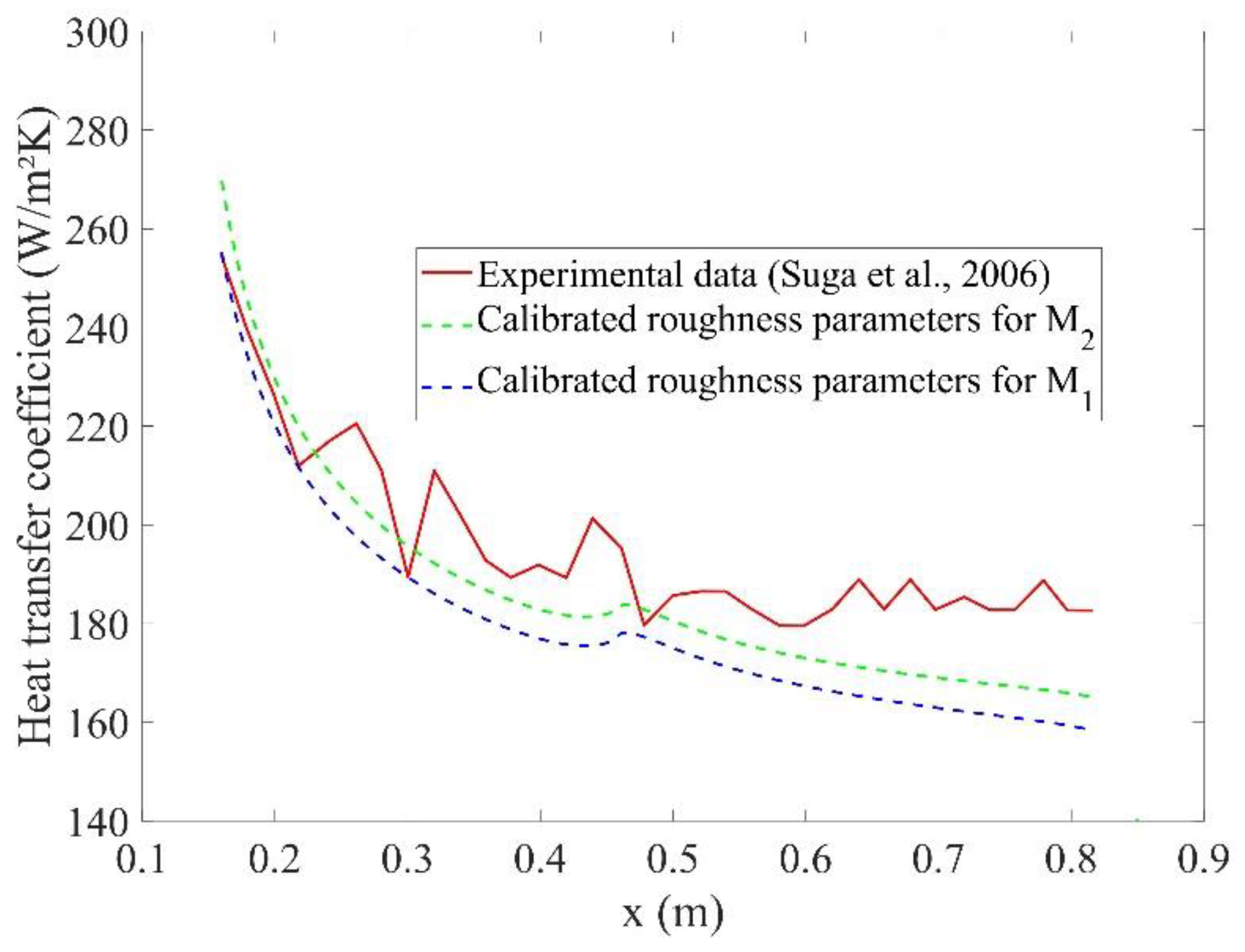
7.5. Bayesian Inversion Calibration

The metamodels built are used as forward models for the MCMC algorithms, evaluated at each iteration of the chain. The target of the calibrations is to retrieve the features of the experimental results by estimating the best roughness parameters. These targets were listed earlier in Table 3. The target values (last column of Table 3) are inputted into the Bayesian module and the computation is carried out on the corresponding metamodel. For metamodels M1 and M2, the calibrated roughness parameters retained are the mean values of the posterior distribution. For metamodel M3, the maximum a posteriori (MAP) is retained. The calibrated roughness parameters retained are listed in Table 7, along with the value (mean or MAP) chosen.
The values in Table 7 are different from the ones tested in the baseline simulation, what explains the poor agreement with the literature prior to the calibration. Before assessing the quality of the calibrations, it is interesting to look at the main power of the Bayesian analysis: transforming the prior probability distributions of the inputs (uniform, see Table 1) into the calibrated posterior distributions, which are closer to Gaussian distributions. Figure 7 and Figure 8 illustrate as an example the prior and posterior distributions for the M3 calibration for both k and ks/k roughness parameters, respectively.
In Figure 7 and Figure 8, it is possible to see the difference from the uncalibrated distributions (prior) to the posterior calibrated distributions. The calibrated values are clearly visible since the distributions are less spread and present peaks. Figure 7 and Figure 8 also allow visualizing graphically the meaning of the mean and MAP values: the mean is the mid value between the distribution’s lower and upper limits, while the MAP value corresponds to the highest peak. From the posterior distributions, it is possible to recover the calibrated values of Table 7 for metamodel M3: k = 1.8 mm and ks/k = 2.8 (i.e., ks = 5.0 mm). The observations highlight that the ratio ks/k (Figure 8b) is finely calibrated with a smaller uncertainty compared to the roughness height k (Figure 7b). The posterior distribution for the ratio ks/k exhibits a narrower peak, typical of a small variance.
For the metamodel M1 and M2, the calibrated roughness parameters from Table 7 are inputted into the CFD solver and the simulation is run to verify the new heat transfer obtained after calibration. Figure 9 shows the heat transfer using the calibrated roughness parameters for M1 and M2.
Figure 9 shows that the calibrated results have a better agreement with the experimental results compared to the baseline simulation of Figure 4. The calibration for M1 allows one to obtain an average relative error with the experimental data of 4.7%. The relative error is computed as the average for the entire rough zone among all the grid points. The experimental data being available at about only 25 locations, the experimental values are interpolated at the grid points to allow the relative error calculation. The calibration for M2 presents similar errors with the experimental data with 4.8% of relative mean error. Globally, both calibrations present satisfactory results, showing less than 5% of error on average compared to the experimental results. The results for the metamodel M1 are higher than the one for the metamodel M2, which is due to the higher roughness parameters in the case of M1. This observation is in accordance with the usual experimental observation, where higher roughness elements lead to an enhanced heat transfer [2].
Figure 10 illustrates the calibrated results using the results for the metamodel M3. Since M3 outputs hc values at different locations, it is possible to use the calibrated inputs to plot both PCE metamodel and CFD predictions.
Figure 10 is informative on several aspects: first, the PCE prediction using the calibrated roughness parameters presents a satisfactory agreement with the experimental data. Second, and most importantly, the CFD prediction is close to the PCE prediction. It allows assessing whether the PCE metamodel is reliable enough to predict a solution, and makes it a less costly and time-consuming tool which can replace the CFD on that particular application. Finally, the calibrated CFD results present a good agreement with the experimental data. The mean relative error with the experimental curve is 5.4%.

7.6. Genetic Algorithm Calibration

The same three metamodels are now calibrated with the genetic algorithm. The objectives of the calibrations remain the same, and the objective functions were listed earlier in Table 4. The calibrated results obtained are displayed below in Table 8. For the metamodel M3, the genetic algorithm outputs N calibrated parameters corresponding to each of the N locations. The final retained parameters are computed by average or weighted average (where the initial point at the start of the rough zone has a weight of three).
Figure 11 shows the CFD results using the calibrated parameters for the metamodels M1 and M2.
Figure 11 highlights that the agreement with the experimental data is better at the beginning of the rough zone and tends to present higher discrepancy at the end of the rough zone. The mean relative error for the metamodel M1 is 8.2% and is 5.7% for metamodel M2.
Figure 12 displays the PCE and CFD predictions using the calibrated values of metamodel M3. The calibration shows better agreement in the middle and at the end of the wall. This feature has a drawback: the agreement at the beginning is not as good as for the metamodels M1 and M2. Taking the average roughness parameters gives a large overestimation of hc at the start of the rough zone. Performing a weighted average, giving a weight of three to the first point, tends to lower the starting hc value and globally lowers the values everywhere.

7.7. Comparison of Both Calibration Methods

After calibrating the metamodels using both Bayesian inversion and genetic algorithm approaches, the first comparison is the capacity for predicting the experimental data. This comparison is made by computing the mean relative error compared with experimental data. Table 9 gathered together the mean relative errors for both approaches.
The Bayesian calibration allows an agreement between the numerical results and the experimental data with an error about 5%. For the genetic algorithm, the errors are higher: they are between 5.7% and 10%. These values show an agreement not as good as the one obtained with the Bayesian inversion, despite displaying interesting behaviour at the beginning of the rough zone for the metamodels M1 and M2 (see Figure 11). By purely looking at the values in Table 9, the Bayesian inversion provides more satisfying and consistent results compared to the genetic algorithm. Note that the uncertainty in the experimental results was not considered. Given the oscillations observed on the experimental curve, one can estimate that the uncertainty in the experimental data is between 6% and 10%.
Nevertheless, by comparing Figure 9, Figure 10, Figure 11 and Figure 12, both methods have their own strengths and weaknesses. The calibrations for the metamodels M1 and M2 present a better agreement at the beginning of the rough zone for the genetic algorithm calibration (Figure 11) compared to the Bayesian inversion (Figure 9). When calibrating the starting value of hc with the metamodel M1, the genetic algorithm performs better since the starting value of hc after calibration agrees better with the experimental data compared to the Bayesian inversion. On the other hand, the Bayesian inversion presents a better agreement between the calibrated results and the experimental data in the middle and at the end of the rough zone. For the metamodel M3, the trend is the opposite: the Bayesian inversion (Figure 10) performs better at the beginning of the rough zone while the genetic algorithm (Figure 12) exhibits a better agreement at the end of the rough zone.
On usage, the Bayesian inversion is more automated and gives a more flexible output. The posterior distribution gives an idea of the uncertainty of the calibrated parameters. In the meantime, the output of the genetic algorithm is more rigid, since apart from the calibrated value, no distribution is given. In the case of a multi-output metamodel (M3), the Bayesian inversion calibrates the model by working simultaneously on all outputs, thus estimating correlated calibrated parameters. The genetic algorithm works on each output independently, and requires a human intervention to establish the correlation between the outputs, like in the case of the weighted-average metamodel M3. Modeller intervention can have a large impact on the results. Table 9 shows that changing the weight of the first output of the metamodel M3 from one to three in the averaging decreases the error from 10% to 7%. An optimization of the weights in the future could improve the results even further.
The novelty of this work resides in the joint application of PCE metamodeling with a calibration method in the field of rough heat transfer prediction. Usually, unknown roughness patterns lead to large uncertainty in the aerothermal behaviour observed. With the methodology presented here, it is possible to reduce the lack of knowledge about a given experimental roughness pattern. As an extension, the present methodology can be applied to aircraft icing, where aerothermal and ice accretion behaviour depend strongly on the initial and uncertain (and unknown) roughness pattern [5,42]. Finely calibrating the roughness parameters in an icing simulation will reduce one source of uncertainty that affects the final prediction of the ice shape.

8. Conclusions

The paper presents a methodology to perform a calibration of roughness parameters aiming at approaching experimental heat transfers. Two methods of calibration were compared: the Bayesian inversion and the genetic algorithm. Furthermore, this methodology was applied to a rough curved channel test case to illustrate its capacity. Starting with an unknown experimental roughness pattern, the procedure allowed the recovery of roughness parameters, providing between 4.7% and 5.4% of discrepancies with the experimental heat transfer when using Bayesian inversion calibration. In the case of the genetic algorithm, the agreement was above 5.7%, reaching 10%. The Bayesian inversion handled better than the genetic algorithm in the present application since its calibrated results fit the experimental data better. Furthermore, the Bayesian inversion behaves better in the case of multi-output metamodels, since it does not require manual tuning to account for each output contribution. This building of this methodology was achieved by combining polynomial chaos expansion (PCE) metamodeling and calibration techniques. The methodology showed high accuracy with respect to the PCE metamodels, confirming their suitability in the current application. The sensitivity analysis using the Sobol sensitivity indices highlighted that for this test case, the relation between the roughness height and the equivalent roughness plays a bigger role than the roughness height alone. The data-driven approach showed its suitability in CFD applications. In the case of unknown roughness patterns, it allows one to select the numerical parameters to input into a CFD simulation to retrieve the experimental data. Future extensions of the work will allow one to calibrate the roughness parameters not only to fit the heat transfer value but related quantities such as ice shape geometry in in-flight icing simulations.

Author Contributions

Conceptualization, K.I., F.M. and H.B.; methodology, K.I.; validation, K.I., E.S., F.M. and H.B.; investigation, K.I.; resources, F.M.; data curation, K.I.; writing—original draft preparation, K.I.; writing—review and editing, K.I., F.M., H.B. and E.S.; supervision, F.M. and H.B.; project administration, F.M. All authors have read and agreed to the published version of the manuscript.

Funding

This research received no external funding.

Institutional Review Board Statement

Not applicable.

Informed Consent Statement

Not applicable.

Data Availability Statement

The data presented in this study are available on request from the corresponding author.

Acknowledgments

The authors want to thank the TOMATO Association (Aéroclub de France), Paris, France, the Office of the Dean of Studies, ÉTS, Montréal, Canada, and SubstanceETS, Montréal, Canada. CFD computations were made on the supercomputer Cedar from Simon Fraser University, managed by Calcul Québec and Compute Canada.

Conflicts of Interest

The authors declare no conflict of interest.

Nomenclature

Symbols
dDistance to the wall (m)
EMean value of a dataset
e a i j Relative error between mesh i and j for a scalar quantity
gAdimensional factor in the thermal correction model
hcHeat transfer coefficient (W/m2K)
kRoughness height (m)
ksEquivalent roughness (m)
lMesh characteristic length (m)
MiMetamodel
NpointsNumber of mesh points in the rough wall
NNumber of outputs for a multi-output metamodel
P r Laminar Prandtl number
pConvergence order for mesh study
pPCEDegree of polynomial chaos expansion
R2Regression coefficient
R e S Roughness Reynolds number
Si and Si,jFirst and second order Sobol indices
STiTotal Sobol index
u τ Friction velocity (m/s)
VVariance of a dataset
xLocal abscissa along the channel (m)
X = (X1,X2) Vector of input variables for a metamodel
YiOutput of interest of a metamodel
yαCoefficient of the PCE term of index α
Greek letters
α = (α12)Multi-index of the PCE decomposition
Δ P r t Turbulent Prandtl number correction
ν Kinematic viscosity of air (m2/s)
εMean relative error
ψ α Multivariate polynomial of index α
φ α i Univariate polynomial of index αi
π(θ|Xi)Posterior distribution of input Xi
π(θ)Prior distribution with parameters θ
π(Xi)Marginal likelihood
Subscripts
CFDCFD-predicted value
EXPExperimental value

Appendix A

This appendix sums up the main results obtained during the mesh convergence study. Three meshes are used for a channel simulation (a coarse (1), a medium (2) and a fine (3) mesh). The roughness parameters used are k = 0.5 mm and ks = 1.55 mm. The mesh convergence methodology suggested by [43] is used to compute the convergence order p and the grid convergence index (GCI). The flow quantities monitored are hc at three locations: x = 0.16 m, x = 0.46 m and x = 0.80 m. The results are gathered in Table A1.
Table A1. Convergence orders and GCI values.
hc (x = 0.16 m)hc (x = 0.46 m)hc (x = 0.8 m)
p0.71.72.1
GCI210.9%0.2%0.1%
GCI321.4%0.7%0.5%
Table A1 shows low GCIs—mainly below 1% except for one which is at 1.4%. For instance, for the monitored hc at 0.8 m on the fine mesh, the interpretation of the GCI value is that the uncertainty on the monitored hc due to the mesh refinement is 0.1%. Applying the same interpretation for each value denotes a satisfactory mesh convergence study. To be conservative and confident about the quality of the CFD results, even with the various roughness patterns planned to be run, the fine mesh is retained for the rest of the process.

References

  1. Aupoix, B.; Spalart, P.R. Extensions of the Spalart–Allmaras turbulence model to account for wall roughness. Int. J. Heat Fluid Flow 2003, 24, 454–462. [Google Scholar] [CrossRef]
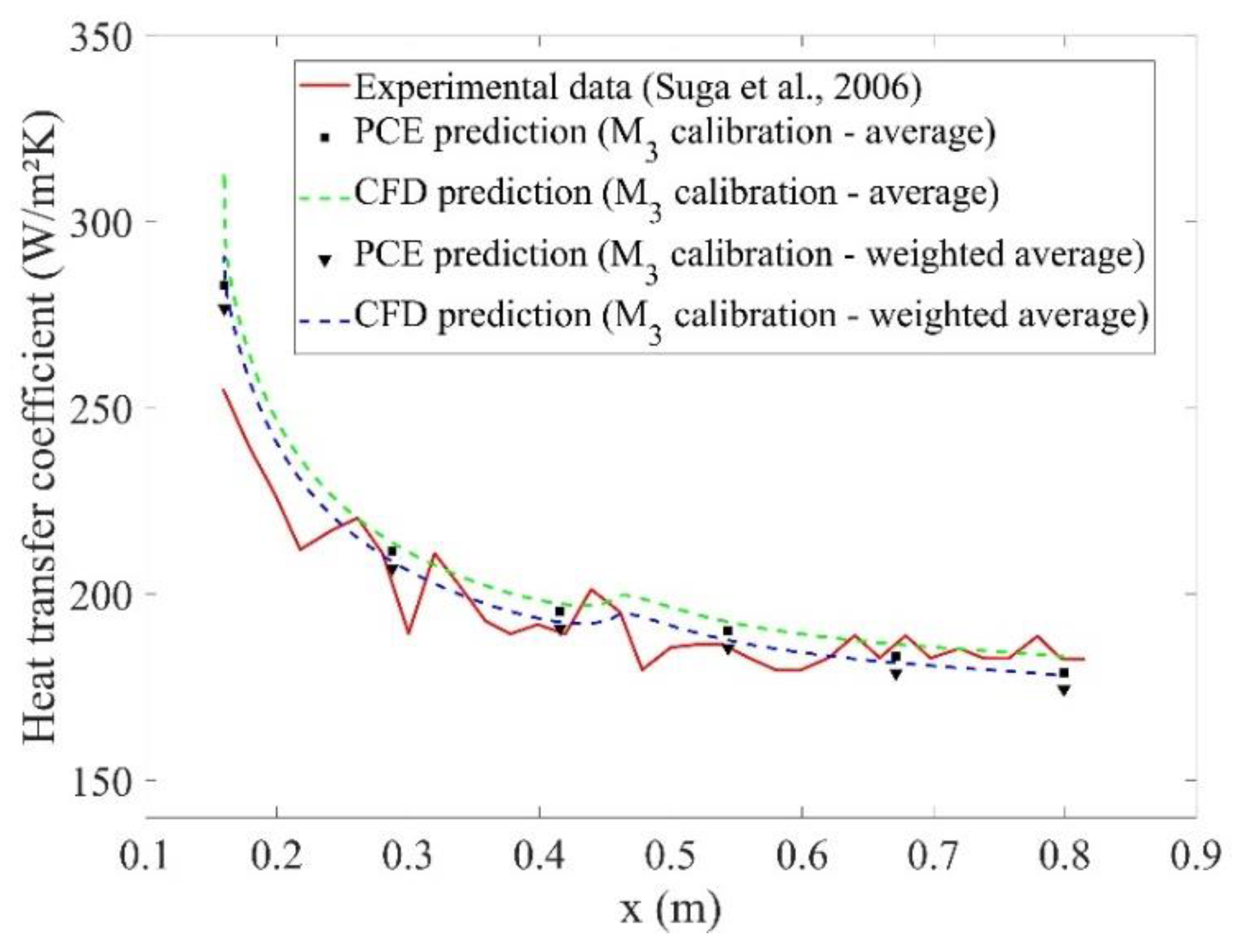
  2. Suga, K.; Craft, T.J.; Iacovides, H. An analytical wall-function for turbulent flows and heat transfer over rough walls. Int. J. Heat Fluid Flow 2006, 27, 852–866. [Google Scholar] [CrossRef]
  3. Aupoix, B. Improved heat transfer predictions on rough surfaces. Int. J. Heat Fluid Flow 2015, 56, 160–171. [Google Scholar] [CrossRef]
  4. Morency, F.; Beaugendre, H. Comparison of turbulent Prandtl number correction models for the Stanton evaluation over rough surfaces. Int. J. Comput. Fluid Dyn. 2020, 34, 278–298. [Google Scholar] [CrossRef]
  5. Ignatowicz, K.; Morency, F.; Beaugendre, H. Sensitivity Study of Ice Accretion Simulation to Roughness Thermal Correction Model. Aerospace 2021, 8, 84. [Google Scholar] [CrossRef]
  6. Dirling, R. A method for computing roughwall heat transfer rates on reentry nosetips. In Proceedings of the 8th Thermophysics Conference, Palm Springs, CA, USA, 16–18 July 1973. [Google Scholar] [CrossRef]
  7. Shin, J. Characteristics of surface roughness associated with leading-edge ice accretion. J. Aircr. 1996, 33, 316–321. [Google Scholar] [CrossRef]
  8. Da Ronch, A.; Panzeri, M.; Drofelnik, J.; D’ippolito, R. Sensitivity and calibration of turbulence model in the presence of epistemic uncertainties. CEAS Aeronaut. J. 2020, 11, 33–47. [Google Scholar] [CrossRef] [Green Version]
  9. Marelli, S.; Sudret, B. UQLab User Manual—Polynomial Chaos Expansions; Chair of Risk, Safety and Uncertainty Quantification, ETH: Zurich, Switzerland, 2019. [Google Scholar]
  10. Salehi, S.; Raisee, M.; Cervantes, M.J.; Nourbakhsh, A. Efficient uncertainty quantification of stochastic CFD problems using sparse polynomial chaos and compressed sensing. Comput. Fluids 2017, 154, 296–321. [Google Scholar] [CrossRef]
  11. Hosder, S.; Walters, R.; Perez, R. A Non-Intrusive Polynomial Chaos Method For Uncertainty Propagation in CFD Simulations. In Proceedings of the 44th AIAA Aerospace Sciences Meeting and Exhibit, Reno, NV, USA, 9–12 January 2006. [Google Scholar] [CrossRef]
  12. Rumpfkeil, M.P.; Beran, P.S. Multifidelity Sparse Polynomial Chaos Surrogate Models Applied to Flutter Databases. AIAA J. 2020, 58, 1292–1303. [Google Scholar] [CrossRef]
  13. Shahane, S.; Aluru, N.R.; Vanka, S.P. Uncertainty quantification in three dimensional natural convection using polynomial chaos expansion and deep neural networks. Int. J. Heat Mass Transf. 2019, 139, 613. [Google Scholar] [CrossRef] [Green Version]
  14. Tabatabaei, N.; Raisee, M.; Cervantes, M.J. Uncertainty Quantification of Aerodynamic Icing Losses in Wind Turbine With Polynomial Chaos Expansion. J. Energy Resour. Technol. 2019, 141, 051210. [Google Scholar] [CrossRef]
  15. Zhang, K.; Li, J.; Zeng, F.; Wang, Q.; Yan, C. Uncertainty Analysis of Parameters in SST Turbulence Model for Shock Wave-Boundary Layer Interaction. Aerospace 2022, 9, 55. [Google Scholar] [CrossRef]
  16. Najm, H.N. Uncertainty Quantification and Polynomial Chaos Techniques in Computational Fluid Dynamics. Annu. Rev. Fluid Mech. 2009, 41, 35–52. [Google Scholar] [CrossRef]
  17. Saltelli, A.; Ratto, M.; Andres, T.; Campolongo, F.; Cariboni, J.; Gatelli, D.; Saisana, M.; Tarantola, S. Global Sensitivity Analysis. The Primer; John Wiley & Sons: Hoboken, NJ, USA, 2008; Volume 304. [Google Scholar] [CrossRef]
  18. Resmini, A.; Peter, J.; Lucor, D. Sparse grids-based stochastic approximations with applications to aerodynamics sensitivity analysis. Int. J. Numer. Methods Eng. 2016, 106, 32–57. [Google Scholar] [CrossRef]
  19. Wagner, P.-R.; Nagel, J.; Marelli, S.; Sudret, B. UQLab User Manual—Bayesian Inference for Model Calibration and Inverse Problems; Chair of Risk, Safety and Uncertainty Quantification, ETH: Zurich, Switzerland, 2021. [Google Scholar]
  20. Muehleisen, R.T.; Bergerson, J. Bayesian Calibration—What, Why And How. In Proceedings of the International High Performance Buildings Conference, West Lafayette, IN, USA, 11–14 July 2016. [Google Scholar]
  21. Guillas, S.; Glover, N.; Malki-Epshtein, L. Bayesian calibration of the constants of the κ-ε turbulence model for a CFD model of street canyon flow. Comput. Methods Appl. Mech. Eng. 2014, 279, 536–553. [Google Scholar] [CrossRef] [Green Version]
  22. Morita, Y.; Rezaeiravesh, S.; Tabatabaei, N.; Vinuesa, R.; Fukagata, K.; Schlatter, P. Applying Bayesian optimization with Gaussian process regression to computational fluid dynamics problems. J. Comput. Phys. 2022, 449, 110788. [Google Scholar] [CrossRef]
  23. Reddy, T.A.; Maor, I.; Panjapornpon, C. Calibrating Detailed Building Energy Simulation Programs with Measured Data—Part II: Application to Three Case Study Office Buildings (RP-1051). HVAC&R Res. 2007, 13, 243–265. [Google Scholar] [CrossRef]
  24. Yang, X.-S. (Ed.) Chapter 6—Genetic Algorithms. In Nature-Inspired Optimization Algorithms, 2nd ed.; Academic Press: Cambridge, MA, USA, 2021; pp. 91–100. [Google Scholar] [CrossRef]
  25. Khan, A.H.; Islam, M.S.; Sazzad, I.U. Calibration of κ-ε turbulence model for thermal–hydraulic analyses in rib-roughened narrow rectangular channels using genetic algorithm. SN Appl. Sci. 2021, 3, 678. [Google Scholar] [CrossRef]
  26. Oh, J.; Chien, N.B. Optimization Design by Coupling Computational Fluid Dynamics and Genetic Algorithm. In Computational Fluid Dynamics—Basic Instruments and Applications in Science; IntechOpen: London, UK, 2018. [Google Scholar] [CrossRef] [Green Version]
  27. Owoyele, O.; Pal, P.; Torreira, A.; Probst, D.; Shaxted, M.; Wilde, M.; Senecal, P. Application of an automated machine learning-genetic algorithm (AutoML-GA) approach coupled with computational fluid dynamics simulations for rapid engine design optimization. Int. J. Engine Res. 2021. [Google Scholar] [CrossRef]
  28. Wagner, P.-R.; Fahrni, R.; Klippel, M.; Frangi, A.; Sudret, B. Bayesian calibration and sensitivity analysis of heat transfer models for fire insulation panels. Eng. Struct. 2019, 205, 110063. [Google Scholar] [CrossRef] [Green Version]
  29. Ranftl, S.; Von Der Linden, W. Bayesian Surrogate Analysis and Uncertainty Propagation. Phys. Sci. Forum 2021, 3, 6. [Google Scholar]
  30. Turner, A.B.; Hubbe-Walker, S.E.; Bayley, F.J. Fluid flow and heat transfer over straight and curved rough surfaces. Int. J. Heat Mass Transf. 2000, 43, 251–262. [Google Scholar] [CrossRef]
  31. Economon, T.D.; Palacios, F.; Copeland, S.R.; Lukaczyk, T.W.; Alonso, J.J. SU2: An Open-Source Suite for Multiphysics Simulation and Design. AIAA J. 2015, 54, 828–846. [Google Scholar] [CrossRef]
  32. Blazek, J. Computational Fluid Dynamics: Principles and Applications, 2nd ed.; Elsevier: Amsterdam, The Netherlands, 2005. [Google Scholar]
  33. Dukhan, N.; Masiulaniec, K.C.; Witt, K.J.D.; Fossen, G.J.V. Experimental Heat Transfer Coefficients from Ice-Roughened Surfaces for Aircraft Deicing Design. J. Aircr. 1999, 36, 948–956. [Google Scholar] [CrossRef]
  34. Fortin, G. Equivalent Sand Grain Roughness Correlation for Aircraft Ice Shape Predictions; SAE International: Warrendale, PA, USA, 2019. [Google Scholar] [CrossRef]
  35. Stein, M. Large sample properties of simulations using latin hypercube sampling. Technometrics 1987, 29, 143–151. [Google Scholar] [CrossRef]
  36. Schaefer, J.A.; Cary, A.W.; Mani, M.; Spalart, P.R. Uncertainty Quantification and Sensitivity Analysis of SA Turbulence Model Coefficients in Two and Three Dimensions. In Proceedings of the 55th AIAA Aerospace Sciences Meeting, Grapevine, TX, USA, 9–13 January 2017. [Google Scholar] [CrossRef]
  37. Degennaro, A.M.; Rowley, C.W.; Martinelli, L. Uncertainty Quantification for Airfoil Icing Using Polynomial Chaos Expansions. J. Aircr. 2015, 52, 1404–1411. [Google Scholar] [CrossRef] [Green Version]
  38. Chan, K.; Saltelli, A.; Tarantola, S. Sensitivity Analysis of Model Output: Variance-based Methods Make the Difference. In Proceedings of the 29th Conference on Winter Simulation, Atalanta, GA, USA, 7–10 December 1997. [Google Scholar] [CrossRef]
  39. Goldberg, D.E. Genetic Algorithms in Search, Optimization and Machine Learning; Addison-Wesley Longman Publishing Co., Inc.: Boston, MA, USA, 1989. [Google Scholar]
  40. Conn, A.R.; Gould, N.I.M.; Toint, P. A Globally Convergent Augmented Lagrangian Algorithm for Optimization with General Constraints and Simple Bounds. SIAM J. Numer. Anal. 1991, 28, 545–572. [Google Scholar] [CrossRef] [Green Version]
  41. Prince Raj, L.; Yee, K.; Myong, R.S. Sensitivity of ice accretion and aerodynamic performance degradation to critical physical and modeling parameters affecting airfoil icing. Aerosp. Sci. Technol. 2020, 98, 105659. [Google Scholar] [CrossRef]
  42. Ignatowicz, K.; Morency, F.; Beaugendre, H. Numerical simulation of ice accretion using Messinger-based approach: Effects of surface roughness. In Proceedings of the CASI AERO Conference 2019, Laval, QC, Canada, 14–16 May 2019. [Google Scholar]
  43. Celik, I.; Ghia, U.; Roache, P.J.; Freitas, C.; Coloman, H.; Raad, P. Procedure of Estimation and Reporting of Uncertainty Due to Discretization in CFD Applications. J. Fluids Eng. 2008, 130, 078001. [Google Scholar] [CrossRef] [Green Version]
Figure 1. Geometry of the curved channel.
Energies 15 03793 g001
Figure 2. Close view on the mesh in the near-wall region: (a) Inlet area; (b) transition straight/curved zone (scale in m).
Energies 15 03793 g002
Figure 3. Iterative convergence of the baseline simulation.
Energies 15 03793 g003
Figure 4. Baseline results before calibration.
Energies 15 03793 g004
Figure 5. Database of heat transfer coefficients obtained with the DOE.
Energies 15 03793 g005
Figure 6. Regression between PCE and CFD predictions for metamodel M2.
Energies 15 03793 g006
Figure 7. Prior (a) and posterior (b) distributions for the roughness height k (M3 calibration).
Energies 15 03793 g007
Figure 8. Prior (a) and posterior (b) distributions for the ratio ks/k (M3 calibration).
Energies 15 03793 g008
Figure 9. Heat transfer coefficient after Bayesian calibration.
Energies 15 03793 g009
Figure 10. PCE and CFD predictions using M3 calibrated values (Bayesian inversion).
Energies 15 03793 g010
Figure 11. Heat transfer coefficient after genetic algorithm calibration.
Energies 15 03793 g011
Figure 12. PCE and CFD predictions using M3 calibrated values (genetic algorithm).
Energies 15 03793 g012
Table 1. Distribution of the input parameters.
ParameterMinimumMaximumDistribution
k (mm)0.414.32Uniform
Ratio ks/k0.26.5Uniform
Table 2. The metamodels created.
MetamodelOutput(s) of Interest
M1hc at the starting point of the rough zone, W/m2K
M2Mean relative error with experimental hc (%)
M3hc values at N equally spaced locations along the rough zone (multi-output), W/m2K
Table 3. Bayesian solver settings.
Metamodel CalibratedObjective of the CalibrationSamplerDiscrepancyExperimental Observation Supplied
M1Recovering the same starting value of hcAIESUniform [0; 15] W/m2K255.1 W/m2K
M2Having a mean relative error with experimental hc of 0%AIESUniform [0; 5]%0%
M3Recovering the same hc values at the N equally spaced locations along the rough zone MHUniform [0; 15] W/m2KExperimental hc at the N locations (W/m2K)
Table 4. Objective functions for calibration with the genetic algorithm.
Metamodel
Calibrated
Objective of the CalibrationObjective Function Used
M1Recovering the same starting value of hc|M1 − 255.1|
M2Having a mean relative error with experimental hc of 0%|M2|
M3Recovering the same hc values at the N equally spaced locations along the rough zone |M3[i] − hc[i]|
i = 1…N
Table 5. R2 coefficient for each metamodel.
MetamodelOutput of InterestPCE Degree
pPCE
Number of Terms in Equation (4)R2
Coefficient
M1hc at the starting point of the rough zone, W/m2K10660.99994
M2Mean relative error with experimental hc (%)10660.99962
M3hc values at 6 equally spaced locations along the rough zone (multi-output), W/m2KY1:10660.99994
Y2:9550.99993
Y3:12910.99999
Y4:10660.99992
Y5:12910.99999
Y6:12910.99997
Table 6. Total Sobol indices.
MetamodelTotal Sobol Indices
M1k: 0.1445
ks/k: 0.8868
M2k: 0.3061
ks/k: 0.9772
M3k: 0.1167
ks/k: 0.9061
Table 7. Calibrated roughness parameters (Bayesian inversion).
Calibrated MetamodelValues RetainedFinal Calibrated Roughness Parameters
M1Meank = 2.2 mm
ks = 6.4 mm
M2Meank = 1.6 mm
ks = 4.2 mm
M3MAPk = 1.8 mm
ks = 5.0 mm
Table 8. Calibrated roughness parameters (genetic algorithm).
Calibrated MetamodelValues RetainedFinal Calibrated Roughness
Parameters
M1 k = 1.9 mm
ks = 3.1 mm
M2 k = 4.3 mm
ks = 8.2 mm
M3Average among the N valuesk = 3.0 mm
ks = 8.3 mm
M3Weighted average among the N valuesk = 2.9 mm
ks = 7.1 mm
Table 9. Errors with experimental data for each calibration.
Calibrated Metamodelhc Mean Relative Error with Experimental Data
Bayesian InversionGenetic Algorithm *
M14.7%8.2%
M24.8%5.7%
M35.4%Avg: 10%
W-Avg: 7.0%
* For M3, Avg: Average among the N outputs; W-Avg: Weighted average.
Publisher’s Note: MDPI stays neutral with regard to jurisdictional claims in published maps and institutional affiliations.

