Quantifying Compressed Air Leakage through Non-Intrusive Load Monitoring Techniques in the Context of Energy Audits

Abstract

Following the recent European directives highlighting the need to increase energy efficiency in the European Union, this work aims to show the possibility of using Non-Intrusive Load Monitoring (NILM) techniques to improve energy audits by estimating the compressed air leakage from a dataset of a tertiary building. The first step towards the reduction of energy consumption is performing an energy audit, in which a detailed analysis of the energy performance is executed. This analysis usually uses on-site measured data by the auditors. However, the time available for these measurements is limited and may not include some modes of operation. One example of that is the quantification of compressed air leaks. This task can be performed by estimating the flow rate during a no compressed air consumption period. However, these periods may not coincide with the auditors’ original schedule. This problem could be addressed by using historical data. Nevertheless, historical data from energy management systems usually are only available for global consumption, and rarely for individual appliances. In this context, a NILM approach would be helpful to enhance energy audits carrying analysis of modes of operation not included in the on-site measurements. In this paper, the leaks are firstly quantified using measurements mostly for benchmarking purposes. The results suggested 62% of leaks in the study case. In a second step, the Factorial Hidden Markov Model (FHMM) was applied to the data. Five typical working days, simulating the context of an energy audit, were used as training data, while one week during vacation time, with no compressed air consumption, was used to quantify the leaks. The results show that it was possible, in the context of an energy audit, to estimate the compressed air leakage using NILM techniques in this dataset with less than a 1% difference when compared to the estimation made with actual measurement. Finally, savings estimations considering the elimination of the leaks were performed, varying between 10% and 100% of the leakage repair. Considering the ideal scenario of complete leaks elimination, the savings would represent around 44% in the compressed air system and 4.75% of the current annual global consumption.

1. Introduction

The European Directive 2012/27/EU [1] emphasized the need to increase energy efficiency in the European Union in order to reach the target of saving 20% of primary energy consumption compared to the 2020 projections. At the same time, the European Council recognized that the exploitation of the considerable potential for increased energy savings in buildings, transport, products and production processes is vital to the achievement of this goal. While the targets set by the 2012 directive were not met in some countries, the European Council has decided to postpone the reduction targets to the year 2030, by the publication of the Directive 2018/2002/EU [2] while increasing the target value. These reduction targets have increased from 20% in 2020 to 32.5% in 2030. In this context, France is one of the countries where the target is farthest from being reached. For example, in 2019, primary energy consumption was still 7% above the forecast for that year, while in Germany the consumption was 2.2% above the target. In addition, in countries like Italy and Portugal, the target was reached in 2019.

Within the challenges of energy transition and the reduction of consumption, the building sector plays a key role. The energy consumed in buildings accounts for a significant share of global energy consumption. In France, according to Bilan RTE 2018 [3], approximately 67.8% of electricity is consumed in buildings, both residential and tertiary.

A first step towards the reduction of energy consumption is the realization of an energy audit. This audit is a detailed inventory of the energy performance of the systems in a residential, tertiary or even industrial environment. An audit makes it possible to become aware of the quality of the energy installations and the daily behaviors and must provide personalized and quantified advice to consume energy in a more rational way. The European Directive 2012/27/EU, effective in France since 2013, already mandates all sectors of companies to perform an energy audit every four years [1].

In addition, the French ELAN law (Evolution du Logement, de l’Aménagement et du Numérique 2018) [4], imposes, beyond the regulatory audits, reductions in energy consumption of the French tertiary sector. Furthermore, the tertiary decree of 2019 [5], specifies the application of the ELAN law to the objectives of reducing the energy consumption of French tertiary buildings, compared to 2010.

A successful energy audit seeks first to identify the major energy consumers, where the highest energy savings potentials lie. In this context, compressed air systems play a key role. These systems are usually among the major energy consumers in a facility. For example, in 2001, compressed air production accounted for 10% of the total electricity consumption of the industrial sector in the European Union [6]. Due to that, even a relatively small saving in a compressed air system may represent a high reduction in consumption. Among the several energy efficiency measures that can be taken to reduce the consumption of compressed air systems, the reduction of the leaks is, most likely, the one with the highest impact [6]. The repair of the leaks ultimately can contribute to the reduction of the operating time, increasing the life span of the equipment, and reducing the modulation of a fixed-speed air compressor, among other things [7].

There are several techniques to detect and quantify the leakage in compressed air systems. Among them is the use of ultrasonic detectors [8,9] and infrared cameras [7,8]. Although these methods are the industry standard to locate the leaks, they are impractical [10] for the leakage quantification, particularly in the context of an energy audit. Therefore, an alternative to quantifying the compressed air leakage in a facility is to monitor the flow rate during a period of no compressed air consumption, such as holidays, vacations or weekends [11]. Nevertheless, most facilities do not have flow rate meters built in the pipeline that allows monitoring during these periods.

One alternative to come around this issue is to estimate the compressed air flow rate from the air compressor’s input power. However, this would demand the auditors’ presence on-site during a period of no compressed air consumption, which may not be included in their schedule. The lack of measurements during a period like that would make it impossible to quantify the compressed air leaks. Furthermore, air compressors are unlikely to be monitored individually, in a way that would be improbable to use historical logged data from this equipment to estimate the compressed air leakage. Nevertheless, historical logged data of global consumption is often available. Thus, if one could extract the air compressor’s input power from historical data on global consumption the estimation of the compressed air leakage would be facilitated. That extraction could be performed using NILM (Non-Intrusive Load Monitoring) [12] techniques, for example. Usually, the application of supervised techniques, such as the one used in this work, needs as much information as possible, such as the power associated with each state, and the frequency of the change between the states, among others, in the training phase. Therefore, one would think that to retrieve the load curve of an air compressor during a no compressed air consumption period from the global consumption, a period like that should be included in the training data. However, if data during periods like that were available to auditors, it could be used directly to estimate the leaks.

Therefore, this work aims to estimate the compressed air leakage in a tertiary building environment, by the application of NILM techniques, especially the Factorial Hidden Markov Model (FHMM) [13], to retrieve the air compressor’s input power from the global consumption data to further estimation of the compressed air leakage in that facility. It uses only five working days of normal operation data for training, which does not include any no compressed air consumption period. The results obtained show that using data just from a normal operation period as training data, it was possible to satisfactorily disaggregate the air compressor power during another operating mode, such as during a no compressed air consumption period, and thus estimate the compressed air leakage. The use of NILM in this context can enhance an energy audit, allowing analysis that was impossible before, due to schedule, for example, and reduce its costs, preventing further on-site visits by the auditors.

The method presented in this work can come as an extension of the current industrial practices. Nowadays, auditors use ultrasonic detectors of infrared images to detect and locate leaks, but the quantification through these techniques is not trivial. On the other hand, the quantification of the leaks using the input power of the air compressors does not allow for the location of the leaks for the repair, only providing an idea of the number of leaks and the potential savings with the repair. Hence, the combination of the two methods comes as a complete solution to the quantification and detection of the compressed air leakage in a facility.

This article is divided into four main sections. In the first one, the introduction and motivation were presented. Section 2 presents the methodology applied. It gathers introductions to energy audits (Section 2.1), methods to detect and quantify leaks in compressed air systems are discussed (Section 2.2), and the NILM technique used in this work, the Factorial Hidden Markov Model (FHMM) [13] (Section 2.3). Section 2.4 presents the link between energy audits, quantification of compressed air leaks, and NILM techniques. Section 3 presents a study case, quantifying the leaks in the compressed air system of a tertiary building located in the French Alps region. Firstly, the leakage is estimated directly by electric input measurements during a no compressed air consumption period. Then, the FHMM technique is applied to the data. The results show that it was possible, based on an energy audit, to estimate the compressed air leakage in this dataset. After that, energy savings reached with the repair of the leaks are estimated, to demonstrate how impactful this energy efficiency measure can be.

2. Methodology

This section presents the methodology applied to quantify the compressed air leakage used in this work. It is divided in three subsections. The first subsection presents how an energy audit usually unfolds. Afterwards, the state-of-art of compressed air leaks detection and which one of the several existent techniques is presented. Then, the NILM technique used in this work, the FHMM, is briefly introduced. Finally, the link between the energy audits, the quantification of compressed air leakage and the use of NILM methods is presented.

2.1. Energy Audits

Energy audits are one way to obtain accurate and objective assessments of how to achieve savings. An energy audit is a process by which a building is inspected and analyzed by an experienced technician to determine how energy is used in it, with the goal of identifying opportunities for reducing the amount needed to operate the building while maintaining comfort levels [14].

There are several types of energy audits, classified by the level of complexity and detail of the analysis performed. The first and less complex type of energy audit is the Benchmarking Audit. It performs a detailed preliminary analysis of the energy consumption and its cost, relying on utility bills, determining benchmark indices, like the ratio between the energy consumption and the surface area in a determined period, usually a year [14].

The second type is the Walk-through Audit. It consists of a quick tour of the facility to visually inspect the target systems. This may include the analysis of energy consumption patterns and provide comparisons to average benchmarks for similar facilities. When the inspection of the target systems shows promising savings potential, this audit can lead to a more complex audit later [14].

The Standard Audit seeks to quantify energy consumption and losses by performing a detailed analysis of the performances of several energy systems. This analysis usually includes on-site measurements, historical data collection, and testing to determine the efficiency of the analyzed systems. Specific energy engineering calculations are applied to determine efficiencies and calculate energy and financial savings based on improvements and changes to each system. As the name suggests and because of its cost-benefit, it is the most common type of energy audit performed. However, when historical data is not available, and the audit relies on on-site measurements, a photo of the operating conditions and the extrapolation for other operating points of the systems may be laborious to obtain [14].

To address this problem, there is a more complex type of energy audit. It relies on computer simulations to predict the consumption that was not contemplated in the on-site measurements phase. The goal is to build a base for a more consistent comparison with the actual energy consumption of the analyzed facility. This baseline is then used to compare the performances achieved with improvements and changes tested in the simulation environment. Due to the time involved in collecting data and setting up an accurate simulation model, this is the most expensive level of energy audit [14].

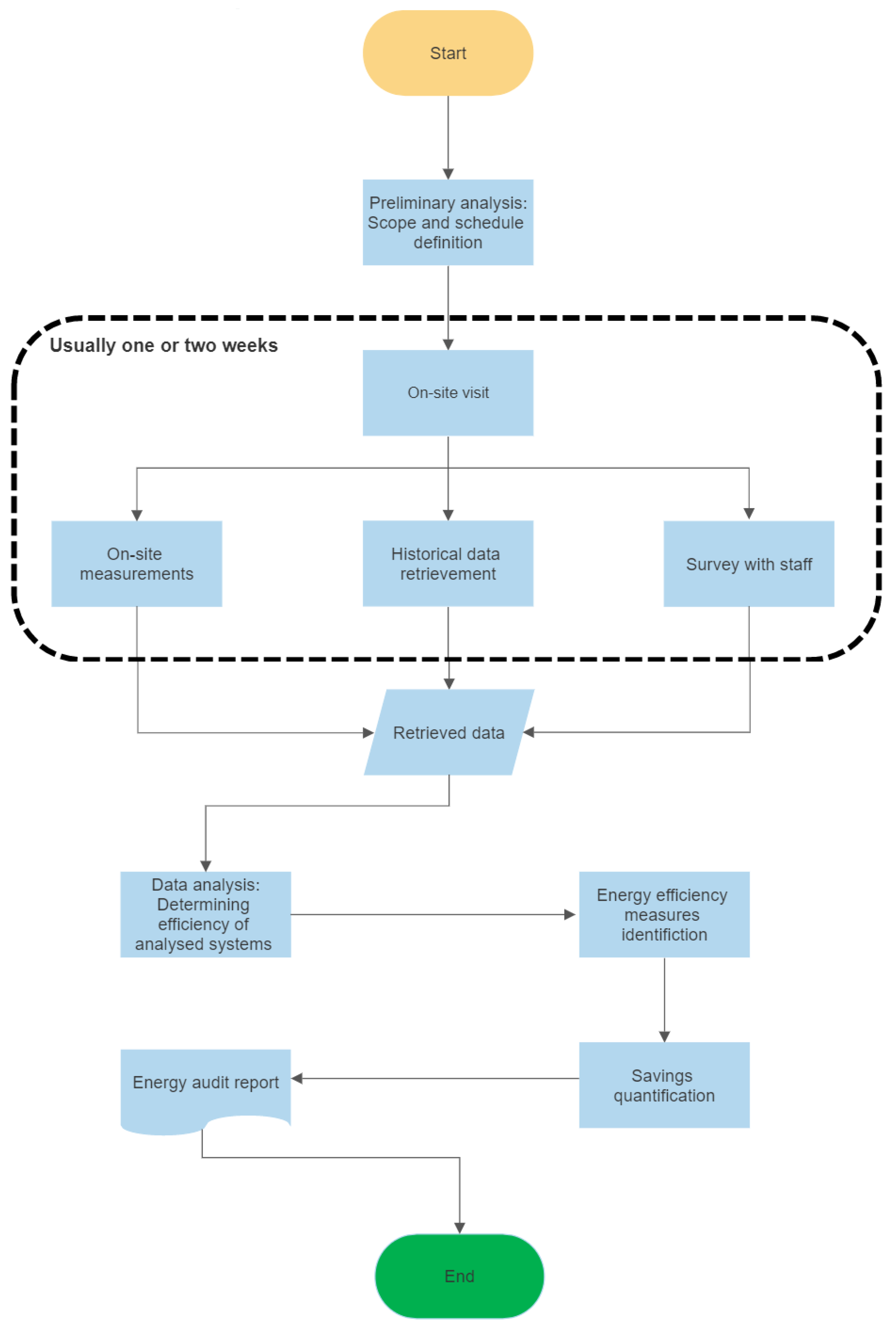
As the Standard Energy Audit is the most common type, the work developed in this paper has been based on it. This procedure can be divided into three phases. The first phase concerns the collection of all necessary data for the efficiency analysis of the evaluated systems. Visual inspections, technical data from catalogs, historical data from the supervisory system, when available, and field measurements are examples of the collected data. This fieldwork consists of taking measurements of various quantities (electrical, thermal, luminous, physical, etc.) necessary to determine the efficiency of the evaluated systems. These measurements should be made following standard technical procedures for each type of system evaluated, using reliable meters adapted to each type of installation and system.

One way to perform this data collection is by incorporating the team into the environment to be evaluated. In this manner, the team can experience the daily operation of the facility. However, besides the fact that the auditors’ time to perform this task is limited, usually a few days or weeks, the ideal is that their activities have as little impact as possible on the normal operation of the systems being evaluated. Due to this, some operating modes of certain equipment may not be measured during the auditors’ data collection period.

The second phase consists of analyzing the collected data and determining the consumption and efficiency of the evaluated systems. To perform this task, the data collected in the preceding phase is applied to procedures specific to each system. In this stage, possible opportunities to promote energy sobriety can also be identified.

The last phase consists of proposing improvements for the reduction of energy consumption, or even the replacement of specific equipment with a more efficient or cheaper one. Replacement by more efficient equipment, changes in operating procedures, or the installation of new components that promote more rational energy are among the most common solutions. All this information is then made available to the customer in the form of a report, in such a way that he can appreciate the alternatives presented and choose whether to make these improvements. Figure 1 illustrates the flowchart process of a standard energy audit.

Usually, large energy consuming systems are the main targets of an energy audit, because even a small absolute reduction in the consumption of these systems can represent large absolute savings. In buildings, lighting systems, HVAC (Heating Ventilation and Air Conditioning), and the envelope are usually emphasized. In industrial environments, besides those mentioned for buildings, analyses in water pumping systems, motors, boilers, and compressed air systems are common.

2.2. Estimating Compressed Leakage

As stated in Section 1, compressed air systems are usually among the major energy consumers in a facility in which these systems are present, whether in a building or an industrial environment. Substitution of a modulating air compressor to a variable speed one, the recovery of the wasted heat, and the quantification and repair of leaks are among the most common and effective solutions to improve efficiency and achieve savings in a compressed air system [6].

Among the energy efficiency measures cited earlier, the repair of compressed air leaks is probably the most impactful energy efficiency measure, applicable to almost all systems. However, the awareness of the importance of a regular leak detection program is usually low, in part because air leaks are invisible, and generally cause no damage [6]. Due to the similar physical characteristics to other gases, the compressed air leakage quantification and detection can be dealt with in an analogous way to other gases. Several methods have been developed to detect and quantify fluid leaks in pipelines. They can be classified into biological, hardware, and software techniques [15].

The biological ones rely on empirical methods using sensorial perceptions, such as the hearing, smell, and sight of specially trained staff. The hardware techniques use numerous equipment to enhance the sensorial perception of the staff. In the case of compressed air systems, the most used are ultrasound [8,9] devices and infrared cameras [7]. Although it is considered the industry standard and best practice, ultrasonic leak detection is limited to the application in short distances [10] and requires highly trained operators. Moreover, due to the compressed air expansion process in the location of the leak, a temperature gradient is created, making it possible to observe it from infrared images. However, these techniques also require the measurement of the openings through which the compressed air escapes from the pipeline to quantify the leaks and thus the potential savings from their repair. The measurement of those openings may be impractical for the auditors. Software-based methods use flow, pressure, temperature, and other data to estimate the leaks. These methods are usually based on the analysis, performed by an automatic algorithm, of both pressure and flow rate data, when available [16,17].

An alternative to quantify the compressed air leakage is to estimate the air compressors flow rate during a no compressed air consumption period. Depending on the facility, a period like that could be weekends, vacations or holidays [11]. During these periods, all the compressed air end use equipment should be turned off. In this scenario all the compressed air is directed to feed only the leaks. This estimation may be done by measuring the input power of the air compressor and correlating it to its flow rate.

This estimation may be done by measuring the input power of the air compressor and correlating it to its Free Air Delivery. There are tables (fixed-speed), and curves (variable-speed) provided by the manufacturers make this correlation possible. When this information is not available, it is possible to measure the flow rate by measuring the air velocity at various points on the intake pipe cross-section and integrate these measurements in the pipe cross-section area, with an anemometer, for example. For the variable-speed compressor, numerous measurements should be done at several operating points, to determine a correlation curve between power and flow rate. The flow rate estimated by correlating the input power of the air compressors, and their free air delivery also enables the determination of the load curve of compressed air in a facility, in the absence of a flow meter.

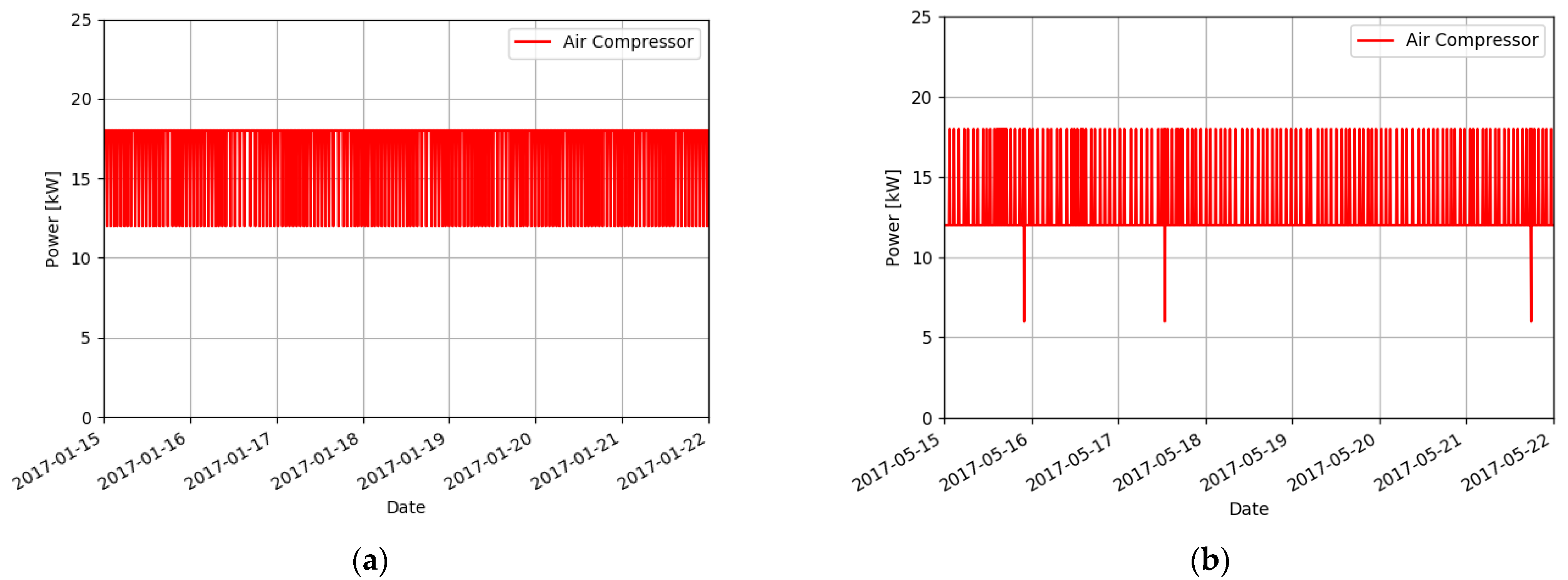
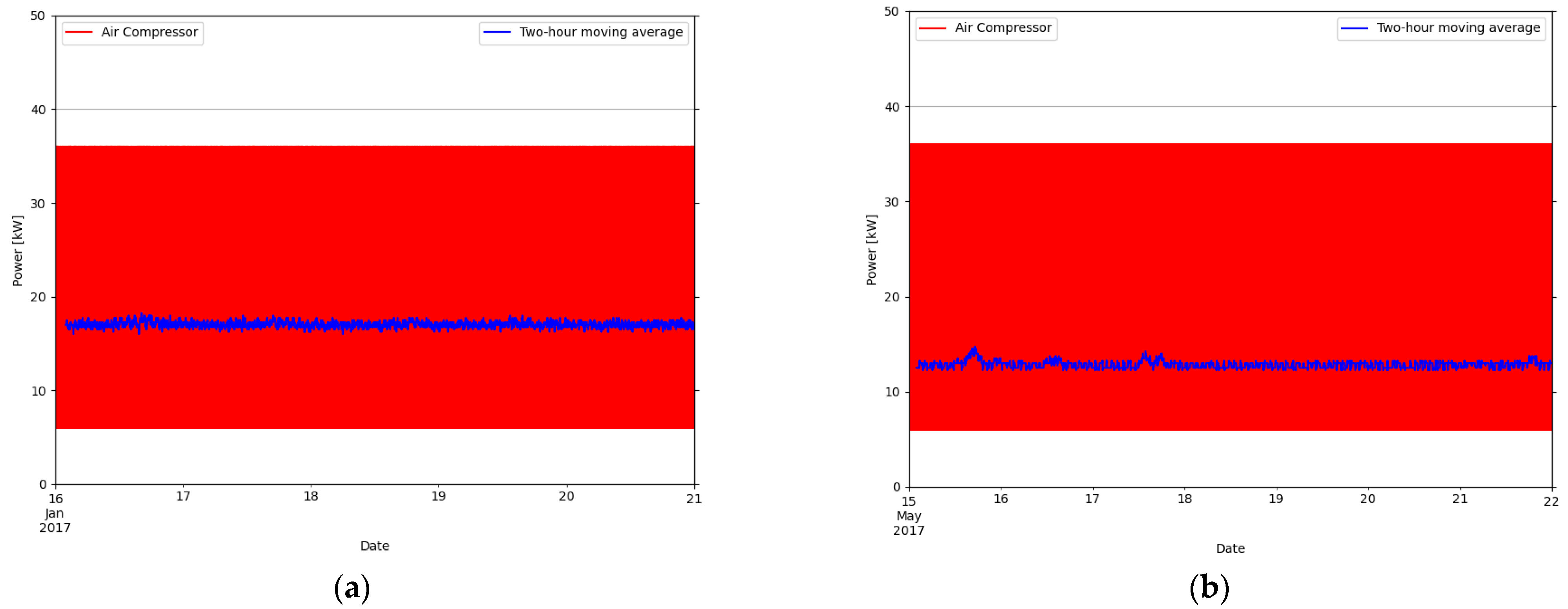
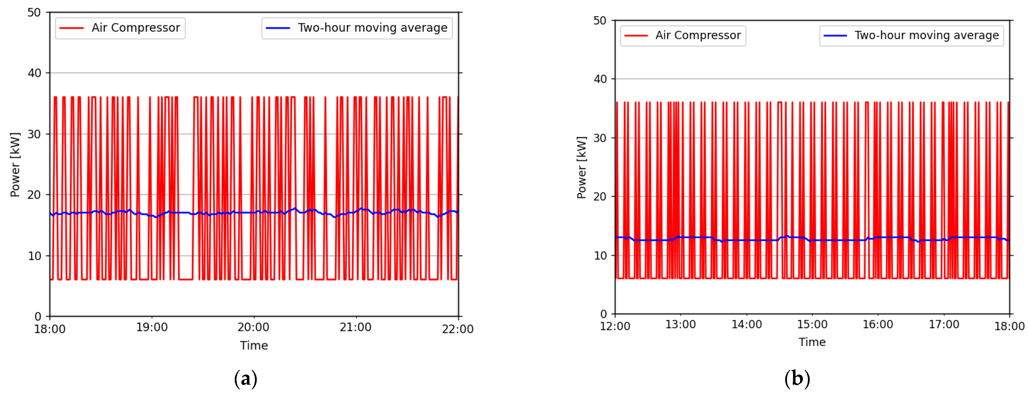
The most common type of air compressor, used in most installations is the rotary screw fixed-speed air compressor. This type of equipment operates at full capacity, the load state, delivering rated flow, until the pressure set point is reached [18]. At this point, the compressor unloads, operating at minimum power, only to maintain internal pressure, delivering no air to the system. Due to this behavior, this type of compressor is also called modulating compressor. These two states, the load and the unload one, typically have very distinguishable input power associated in a way that is not difficult to identify them.

Therefore, to estimate the flow of a rotary screw fixed-speed air compressor it is enough to identify its load state well and correlate it with the compressor’s flow rate capacity, either measured, or obtained from manufacturer tables. For the unload state, zero flow is assigned. Hence, the average flow of a rotary screw fixed-speed air compressor depends directly on how long the equipment remains in its load state. An example of a performance table of a rotary-screw fixed speed air compressor operating at rated pressure provided by the manufacturer is presented in

Table 1. Example of a manufacturer performance table of a fixed-speed air compressor. Based on BelAir datasheet [19].

Model	GS30B10
Manufacturer	BelAir
Rated Capacity at Full Load Operating Pressure [m3/h]	294
Full Load Operating Pressure [bar]	8
Drive Motor Nominal Rating [hp]	40
Total Package Input Power at Zero Flow [kW]	-
Total Package Input Power at Rated Capacity and Full Load Operating Pressure [kW]	33.8

.

As mentioned earlier, one way to quantify compressed air leaks is to estimate the air compressor’s flow rate during a period of no compressed air consumption. However, this technique implies that the auditors must be on-site during a no compressed air consumption period for the monitoring of the air compressors. In an industrial environment, for instance, a no compressed air consumption period is rare, and it may not coincide with the energy audit planning. An alternative route around this problem would be collecting logged data from the compressed air system. However, it is unlikely that the input power of the air compressor, or even the flow rate, is monitored individually. Although it is improbable to have the air compressor’s data logged individually, logged data from the global consumption is often available.

As the correlation between the input power and the flow rate of an air compressor is an intrinsic characteristic of the equipment, it remains the same regardless of the system’s operation mode. Thus, if one could extract the air compressor’s input power from the global consumption, the leakage estimation could be performed even without the presence of the auditors on-site during a no compressed air consumption period. This would enhance the quality of the analysis performed during the energy audit with a smaller cost where the other options for this analysis are impractical.

The load curve extraction of equipment from the global consumption can be done using NILM (Non-Intrusive Load Monitoring) techniques [12] under certain circumstances. Thus, this work aims at investigating the possibility of using NILM methods to estimate the compressed air leakage in a tertiary building environment and to calculate the potential savings with the leaks repair in the context of an energy audit.

NILM techniques have already been used to detect leaks in compressed air systems. In his master thesis [20], Piber used a stationary device to measure the global consumption of a warship. With embedded NILM algorithms, this device was also capable of extracting the consumption of some loads, such as the vacuum-assisted sewage collection system, low pressure compressed air system. Analyzing the operating schedule, he was able to detect the presence of leaks in the compressed air system. However, he did not mention the sampling rate nor the training period used to train the NILM algorithms. In addition, as a stationary device was installed, a permanent change in the facility must be made. So, it is important to highlight that the proposed technique is non-intrusive and does not imply any permanent changes in the system, such as installing flow meters in the pipeline, or stationary power meters.

In summarizing, the idea is to use input power measurements that can be retrieved using portable power analyzers, for instance, to train the algorithm, and logged data from the global consumption to extract the air compressor’s power consumption.

The NILM technique to enhance energy audits was already discussed by Berges et al. [21], but it was limited to application in a residential environment. So, to this date, the authors have not found other methods that relate to the quantification of compressed air leaks through the application of NILM techniques to enhance energy audits in tertiary buildings or in an industrial environment in the literature.

2.3. NILM Techniques

As already mentioned before, in the context of an energy audit, the measurement campaign on-site lasts, usually, a few days or weeks. This phase may not include a no compressed air consumption period, in which the air compressors would operate only to feed the leaks present in the grid. In addition, air compressors are not always monitored individually by a supervisory system, which would make it possible to use historical operating data to estimate the energy consumption, and, consequently, the air leakage during this period. However, it is common to have historical data of the global load curve of the facility, or even of some transformers in substations internal to the facility. In this way, the use of NILM techniques could come as an aid for estimating leakage from this available historical data.

The initial NILM approach was proposed by Hart in the early 1990s in his work entitled “Nonintrusive appliance load monitoring” [12], regarding the residential sector especially. In earlier works, the disaggregation problem was addressed mainly in the residential environment. In these cases, there are fewer appliances and the switch between the on and off states is rare and the power of the equipment in each state is, normally, constant. Therefore, in the disaggregation context, to estimate the consumption profile of an appliance, it is sufficient to know when every piece of equipment works in each state of operation. In his incipient work, Hart [12] proposed a method, nowadays called the Combinatorial Optimization, which consists of finding the combination of the consumption of all appliances in a given instant that minimizes the difference between this combination and the overall ground truth consumption. This method was idealized considering that the appliances operate with finite states, with constant consumption in each one of them. Another commonly applied algorithm is the Factorial Hidden Markov Model [13], which is used in this work.

Several other algorithms try to address the NILM problem, based on different techniques. Some of them are based on Artificial Neural Networks, using recurrent networks [22,23] or convolutional ones [24] or even incorporating the Fourier transform into neural networks to perform the energy disaggregation task [25]. These algorithms have the limitation of performing the energy disaggregation task either with the delay of a few minutes or only for past events. Due to that, the real-time application of NILM models is a recent direction taken by several researchers. For example, Athanasiadis et al. [26] developed a framework combining an event detector, to detect the moment when an appliance changes its state, a convolutional neural network classifier, determining if this state change was caused by a target appliance and a power estimation algorithm to calculate the appliance power and consequently its energy consumption. Later on, a similar framework can be embedded into simple microprocessors to perform on-site energy disaggregation [27].

Although the real-time application is promising, even in the context of an energy audit, a period of no compressed air consumption is needed to quantify leaks. If a period like that is too far in the future, it could delay the deadline of the energy audit report. That is the reason why it was decided to use logged data and the FHMM to perform the estimation.

The Factorial Hidden Markov Model is based on Markov chains. A Markov chain is a stochastic process with discrete or continuous state space that presents the Markovian property. This property states that in regular and discrete time intervals, this stochastic process evolves from one state to another depending only on its last condition, independently of the others.

The Hidden Markov model comes as an extension of the Markov chain. This model includes the case in which the observation is a probability function of the state, i.e., the resulting model is a double-layer stochastic process, in which one stochastic process is underlying and unobservable (hidden) that can only be observed by the other stochastic process that produces the sequences of observations. Due to its flexibility and the simplicity and efficiency of its parameter estimation algorithm, the hidden Markov model (HMM) has emerged as one of the basic statistical tools for modeling discrete time series, finding widespread application in the areas of speech recognition [28] and computational molecular [29].

The disaggregation problem tackled by the FHMM in this work is to infer:

• $\begin{array}{c}\begin{array}{c}{Q}^{\left(1\right)}=\left\{q_1^{\left(1\right)},q_2^{\left(1\right)},\cdots ,q_T^{\left(1\right)}\right\}\\ \begin{array}{c}{Q}^{\left(2\right)}=\left\{q_1^{\left(2\right)},q_2^{\left(2\right)},\cdots ,q_T^{\left(2\right)}\right\}\\ ⋮\end{array}\end{array}\\ Q^{\left(M\right)}=\left\{q_1^{\left(M\right)},q_2^{\left(M\right)},\cdots ,q_T^{\left(M\right)}\right\}\end{array}$ as the power load of each of the M appliances,
• Such that $y_t=\sum _{i=1}^M{q}_t,$
• Given $Y=\left\{y_1,y_2,\cdots ,y_T\right\}$ as the aggregated power for T time periods [30] as the sequence of observations.

An HMM is essentially a mixture model, encoding information about the history of a time series in the value of a single multinomial variable—the hidden state—which can take on one of K discrete values. The system is characterized by this internal discrete state variable, which evolves as a Markov chain between time points. Formally, an HMM can be defined by:

• The finite set of hidden states $S=\left\{S_1,S_2,\cdots ,S_K\right\}$,
• The matrix representing the probability of transitioning from one state to another $A=\left\{a_{ij},1\le i,j\le N\right\}$, being $a_{ij}=P\left(q_{t+1}=S_j|q_t=S_i\right)$ with $a_{ij}\ge 0$ and $\sum _{j=1}^M{a}_{ij}=1$,
• The initial state probability distribution $\pi =\left\{{\pi }_i\right\}$, being ${\pi }_i=P\left(q_1=S_i\right)$

An extension of the HMM is the Factorial Hidden Markov Model (FHMM) [13]. The FHMM extends the HMM by representing the hidden state in a factored form, as $q=\left\{q^{\left(1\right)},q^{\left(2\right)},\cdots ,q^{\left(M\right)}\right\}$ represents the set of underlying state sequences, where $q^{\left(i\right)}=\left\{q_1^{\left(i\right)},q_2^{\left(i\right)},\cdots ,q_T^{\left(i\right)}\right\}$. This way, the information from the past is propagated in a distributed manner through a set of parallel Markov chains. The parallel chains can be viewed as latent features, which evolve over time, according to Markov dynamics. Then, an optimization approach minimizing the difference between the observable variable (global power) and a combination of the hidden states is applied; the complete formulation was developed by Kolter and Jaakkola and it is available in [13].

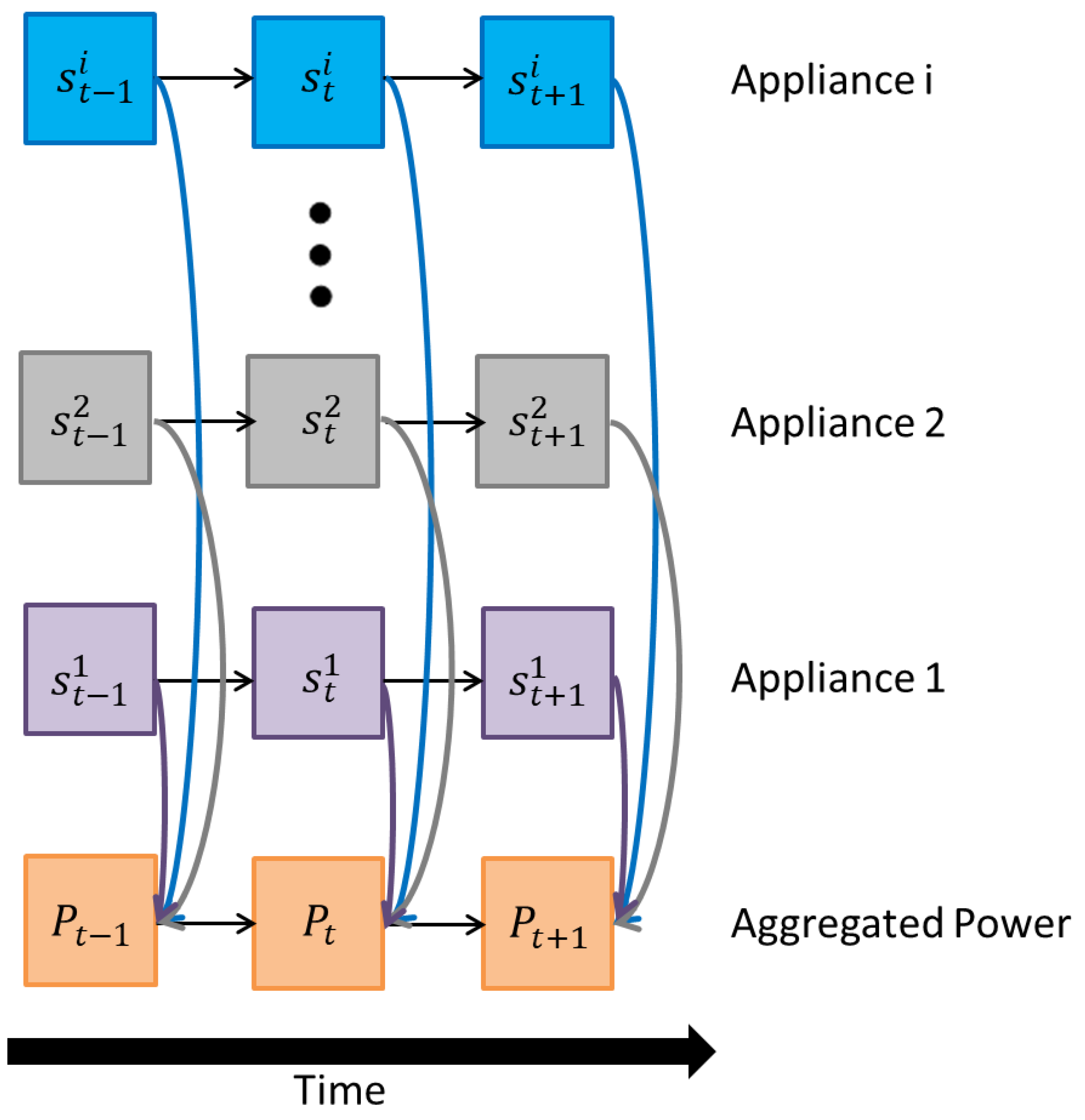
The FHMM applied to solve the NILM problem has been proven to have a good effect on the disaggregation of residential load with a low sampling rate such as 1/60 Hz. It does not directly output the observations of each hidden Markov chain, but outputs the sum of the observations. For the NILM problem, the total active power or reactive power is the observation sequence and the state and power consumption of each piece of equipment is unknown, but the power associated with each state is known. Therefore, each piece of equipment can be described as an HMM, and the working state of the appliance is a Markov chain. The total power is the sum of the power of each appliance, hence, it can be described as an FHMM composed of multiple HMMs, and the observation sequence of the FHMM is the power consumption. In other words, the FHMM tries to predict the combination of active appliances’ energy usage that contributes to global consumption. Figure 2 illustrates how the FHMM is used in the NILM context.

The FHMM was elected to be used in this work because of its simple implementation, fast calculating time, and good performance when dealing with simple and moderate complex loads, such as a rotary screw air compressor addressed in this work. However, the FHMM is not the most suitable algorithm to tackle the NILM task in the presence of more complex loads, such as multi state appliances, or continuously variable loads [32].

2.4. Estimating Compressed Air Leakage in the Context of an Energy Audit

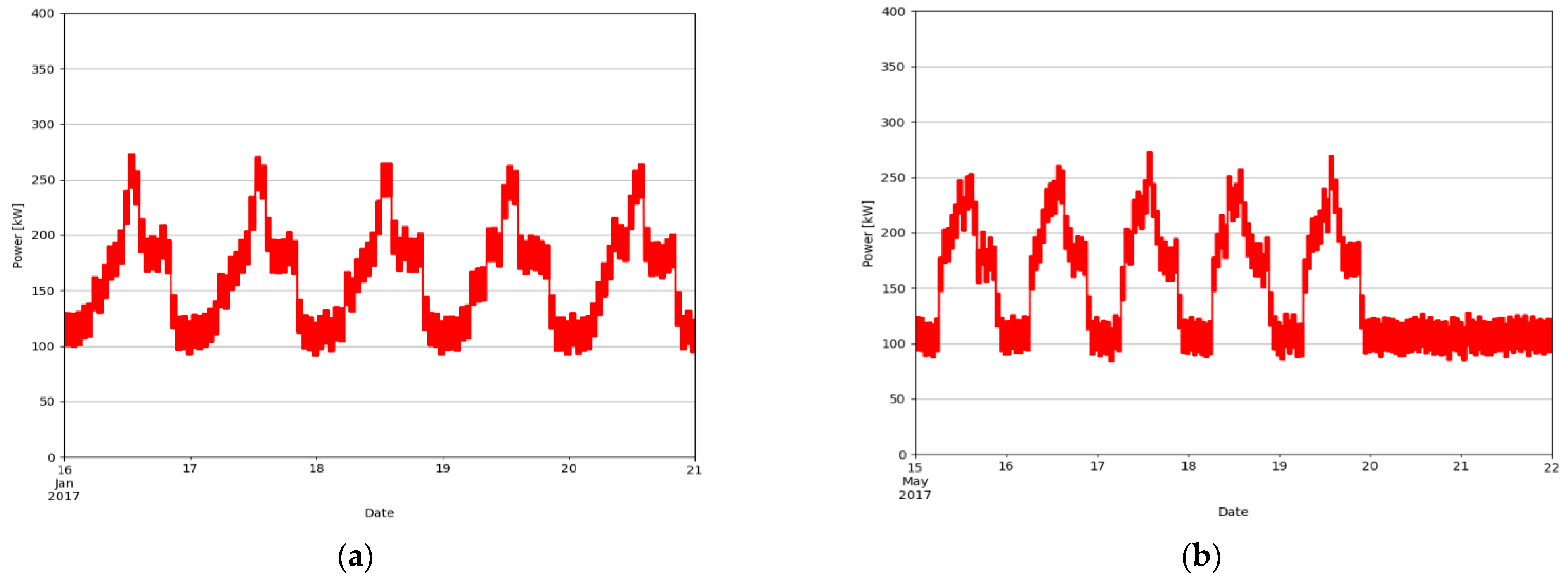
As already stated in previous sections, compressed air systems are usually among the major energy consumers in a facility, and because of the capillarity of their grid, several leaks may appear because of worn out piping and connections. In poorly maintained systems, the leakage can rise to more than half of the total compressed air generated by the air compressors, representing a great opportunity for energy efficiency measures.

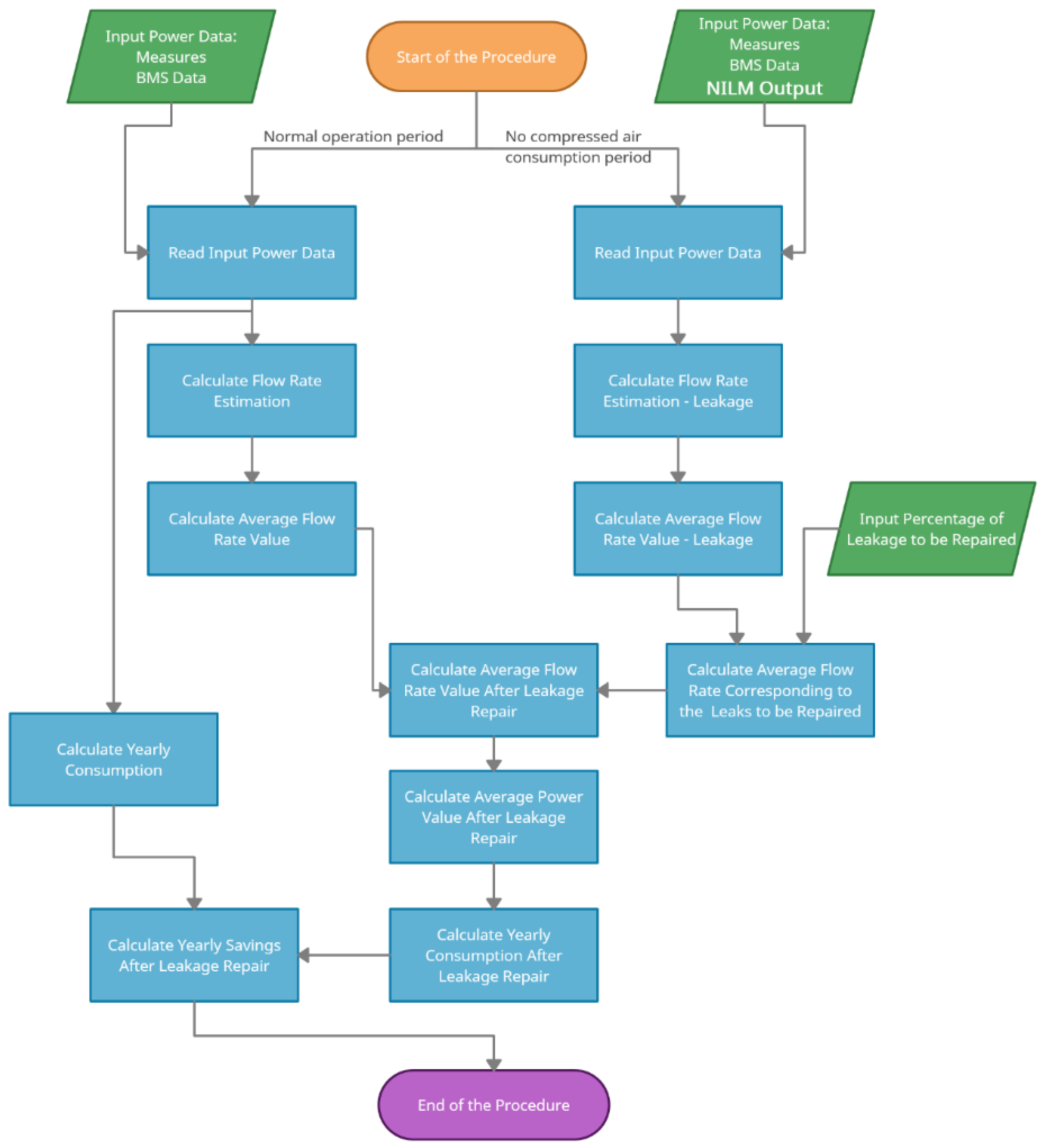
In the absence of monitoring by some management system, which is the typical condition in a facility, the compressed air flow rate can be estimated from the measurement of the air compressor power, and the later determination of its load curve, by the application of the procedure presented in Section 2.2. This estimation, if performed in a period with no compressed air consumption (weekends, vacations, holidays…), represents the leakage present in the grid. If the amount of the leakage is known, the estimation of the savings achieved with the repair of the leaks is feasible. Thus, with input power data, during both normal operation and no compressed air consumption periods, along with the datasheets of the equipment, it is possible to estimate the potential saving by repairing the leaks present in the compressed air system.

However, during a standard energy audit, the auditors normally have only a few days, or a week, to find potential savings and to collect the data needed to perform the calculations, and no compressed air consumption periods may not be included in the auditors’ schedule. Besides that, monitoring and logging data from air compressors individually is unusual. Thus, without the data from a period like that, it would be impossible to satisfactorily estimate the number of compressed air leaks in the grid.

Even if it is unusual to log individual data from air compressors, the load curve of the global consumption is often available. Hence, one way to go around this limitation is to extract, through the application of NILM techniques, air compressor’s load curves from the global consumption.

Figure 3 presents the procedure to estimate compressed air leakage and energy savings with its repair. It shows that would be possible to use the NILM output as power data input during a no compressed air consumption period.

3. Results and Discussions

This section presents a study case of the quantification of compressed air leakage in a tertiary building environment. Firstly, the leaks are quantified by applying the procedure presented in Figure 3, using BMS data available for benchmarking. In a second moment, the FHMM NILM technique is applied to the global consumption of the building, and its output is used to also quantify the leaks. Finally, an analysis of the potential savings with the repair of the leaks is presented.

3.1. Study Case—Estimating Compressed Air Leakage in a Tertiary Building Environment

In order to perform an estimation of compressed air leakage in a facility using NILM techniques, consumption data from a rotary-screw fixed-speed air compressor were extracted from a dataset of a tertiary building located in the French Alps region that is available for downloading in open source at the open science platform Mendeley Data [33]. The data come in CSV (comma-separated values) files that contain the timestamp and the cumulative electricity consumption with 10 min sampling. The dataset also has files with data on the external temperature, which has an influence on the building’s energy consumption because of the nature of the cooling loads. The computational code was developed in Jupyter Notebooks, an environment in python that combines code, text, and images. It is also available in open source [34]. The original data, especially the global consumption, contain some data quality problems, such as the presence of outliers. These anomalous values were identified using the forecast error method [35] and corrected.

The building from which the data were extracted is called GreEn-ER. This building is in the Polygone Scientifique, at the Presqu’île of Grenoble, in France. It gathers the Grenoble-INP engineering school Ense3, the G2Elab laboratory, training, and research platforms. The building has more than 22,000 m² of floor space, which is divided into six floors and a roof. There are about 1500 students and hundreds of professors, researchers, and staff using it. There are more than 1500 m, including more than 300 electricity consumption ones. The other meters concern internal and external conditions, thermic energy data, etc. The measured data are used to control the internal conditions, regarding the comfort of the occupants and to monitor the consumption [36,37].

In order to simulate the context of an energy audit, the period used as training data corresponds to five working days during a normal operation period. A week during vacation time, when there was no use of compressed air, is used to estimate the leaks, corresponding to the test period. The data are sampled at 10-min intervals. The following sections present the estimation of the compressed air leaks using measurement data, for benchmarking the proposed technique, and by the application of the FHMM NILM technique.

3.1.1. Leakage Estimation from Measurements

To estimate compressed air leakage, the procedure presented in Figure 3 was applied using the BMS data available. The scheme of the compressed air production in the building is illustrated in Figure 4. In this figure, it is possible to observe, that there are two air compressors, of which one normally operates while the other is kept as a system backup. Its data sheet was presented in Table 1. The energy consumption raw data corresponds to cumulative energy sampled at 10-min intervals. However, in order to estimate the compressed air flow rate, the cumulative energy data needs to be transformed into power. This can be done by subtracting subsequent samples. The results of the transformation of cumulative energy consumption of the air compressor in both training and test periods, into power, are presented in Figure 5. In this figure, it is possible to identify two main states. The state with associated power of 18 kW was considered the load one while the unload state was associated with the 12 kW value.

In the case of the air compressor installed in the GreEn-ER building, the actual power associated with the load and unload states are different from the values retrieved from Figure 5. Actually, from direct power measurements, the power associated with both load and unload states are 36 kW and 6 kW, respectively, which slightly differs from the value presented in Table 1, probably considering also the dryer power. The difference between the power values associated with each state, and the values directly measured indicates that the air compressor changes its operating states at a greater rate than the sampling interval used. When transforming the energy consumed in the sampling interval into power, an average value is retrieved. However, when this average value does not match the powers associated with the load and unload states (36 kW and 6 kW, respectively), the estimation of the flow rate is affected, since it relies on how long the air compressor remains in each state. Due to that, during the periods in which the air compressor remains in the 18 kW state the flow rate is overestimated and it is underestimated during the 12 kW condition. Due to that, the up sampling to 1-min sampling rate was performed, considering the actual power values (36 kW and 6 kW) associated with each operating state. The choice to resample the data to the 1-min interval was based on how a modulating compressor works, since it is unusual for this type of compressor to switch between the load and unload states at a sub-minute resolution. Furthermore, as the up sampling was performed considering the actual power values associated with each state, and the most important feature to estimate the compressed air flow rate is how long the appliance remains in its load state, higher resolutions, such as 1-s time step, or even sub-second resolution, would not improve the estimations.

In order to up sample the air compressor data keeping the original average power value, it is necessary to determine how much time the compressor operates in each state. For each 10 min period that the compressor presents 18 kW of average power, it has operated for 4 min in load condition (36 kW) and 6 min in unload condition (6 kW). For each 10 min period in which the air compressor power was 12 kW, the asset has operated for 2 min in load conditions and 8 min in unload state. The load and unload operating conditions during the 10 min period were distributed in a random way. Figure 6 shows the air compressor power data, up sampled into 1 minute intervals, during the training and test periods, as well the two-hour moving average for better visualization. At the same time, Figure 7 presents a zoom in of those figures to better visualize the different operation patterns of the air compressor during these two periods.

The up sampling of the data modifies the duration of the period in which the air compressor remains in load state. Consequently, the flow rate estimation drastically changes. With the 10-min sampling interval, most of the time during the training phase the air compressor remained in the load state. However, with the up sampling to 1-min intervals, one sample that was in load state in the 10 min sampling, belongs only 40% of the time now in this condition. So, it is expected that the flow rate estimation decreases. This is confirmed by the values presented in

Table 2. Average air compressor power and flow rate during the different operation periods.

Sampling Interval	Evaluated Period	Number of Samples		Average Value
		Load	Unload	Power [kW]	Flow Rate [m3/h]
10 min	Training Period	846	163	17.03	246.51
	Test Period	140	869	12.83	40.79
1 min	Training Period	3706	6375	17.03	108.08
	Test Period	2296	7785	12.83	66.97

. This table shows the number of samples in which each of the operating states of the air compressor was identified. In addition, using the procedure presented in Section 2.2 the flow rate load curve was then estimated. The same table exposes the average power and estimated flow rate for the normal operation and no compressed air consumption periods for both sampling intervals.

The flow rate estimation presented in Table 2 for 1 min sampling interval matches better to the air compressor characteristics when compared to the estimation for 10 min sampling intervals. With 1 min sampling intervals, the average power represents around 52% of the rated power, while the flow rate estimation represents 36.8% of its rated value. At the same time, the same average power represents around 84% of the rated flow rate for the 10 min sampling data, which is incoherent. Assuming that the 1 min sampling estimation is more accurate, the compressed air leakage represents 62% of the average flow rate during a normal operation period. However, 62% represents a high value of leakage, even in poorly maintained environments, and may suggest other problems, such as irrational usage of compressed air, non-optimal control, usage, etc. Nevertheless, even if this estimation represents more than the leaks, it lends itself to a more detailed investigation.

3.1.2. Leakage Estimation from NILM Techniques

The leakage estimation presented in the previous section was done thanks to the availability of power consumption data in a no compressed air consumption period. However, that is not the typical case in the context of an energy audit. Usually, only the historical data of the global consumption is available, and the auditors have only a few days or weeks of data from the air compressors that were measured by themselves. In addition, it is unusual that the on-site measurement period contains a no compressed air consumption one. Therefore, the use of NILM techniques to retrieve the air compressor’s power from global consumption would allow the quantification of compressed air leaks in such circumstances.

To address this task, the FHMM NILM algorithm was applied with the help of the NILMTK [38,39], an environment in Python developed to enable the comparison between several state-of-art approaches. Hidden Markov models can be used in the NILM context as both supervised (using labeled data to train the algorithm) and unsupervised learning approaches, based on the requirements [13]. In this work, the supervised approach is employed. So, in this approach, FHMM takes some period for the training of the model, to identify power values associated with each state of operation of the target appliances.

In NILM applications, it is typical to select a long period to train the algorithms and create the model, and use a few days as a testing period. For example, in a residential environment study, Batra et al [40] selected two months’ worth of data to train the algorithm while the selected testing period was 10 days. In this paper, the training period of five working days was selected to match the typical time interval that the auditors remain on-site for measurements in order to simulate an energy audit. A week, during a no compressed air consumption period, was selected for testing the model.

Some major consumers were selected in order to create a sub dataset regarding these loads; the global consumption and the air compressor. This sub dataset is used in the NILM task. Five major consumers were selected, and they are named as follows:

• Crous—The Crous load belongs to the University Restaurant, where some typical loads are connected, such as dishwashers, dryers, furnaces, heaters, etc.
• ASI—The ASI load represents loads connected to the datacenter, such as computers, uninterruptible power supply, etc.
• TD-GF—The TD-GF represents chillers that are responsible for the air conditioning during the summer;
• AHU—The load called AHU represents a set of 16 Air Handling Units present in the building;
• Ghost—This load is inserted as noise, and it corresponds to the difference between the main load and the sum of the other loads.

As the sampling interval of the dataset was originally 10-min, all these loads were up sampled to 1 min sampling intervals using forward fill, to match the sampling interval of the air compressor. Figure 8, Figure 9 and Figure 10 illustrate the load curves of the loads described above and the global consumption, during the period used for the training and the period used to estimate the leaks.

Table 3. Average power of the loads.

Load	Average Power [kW]
	Training Period	Test Period
Main	143.67	139.98
Crous	20.99	21.07
AHU	27.00	32.77
TD-GF	5.32	0.48
ASI	38.11	38.06
Ghost	35.18	34.78

presents the average power of these loads during both periods. The air compressor load curves were already shown in Section 3.1.1.

Using the NILMTK framework, the FHMM algorithm was then applied. The algorithm uses the training data to model the loads into finite states and associates each state with an electric power value.

Table 4. Number of states used to model each load and power associated to them.

Load	Number of States Used to Model the Load	Power Associated to State
Crous	5	10.0
		11.0
		25.0
		49.0
		72.0
TD-GF	5	1.0
		4.0
		6.0
		8.0
		15.0
Ghost	4	33.0
		35.0
		36.0
		37.0
ASI	3	36.0
		38.0
		39.0
AHUs	3	4.0
		25.0
		71.0
Air Compressor	2	6.0
		36.0

presents the number of states that the FHMM uses to model each load and the power associated with them.

Therefore, applying the formulation detailed in [13] to the data it is possible to infer the individual consumption of each appliance. The results presented in Figure 11 illustrate the disaggregation output using the FHMM for the air compressor load, the main target of this work. In this figure, GT means Ground Truth, or the actual consumption, and FHMM are the results from the FHMM NILM algorithm.

It can be seen in the previous figure that the FHMM algorithm was able to retrieve most of the air compressor consumption in this example. In order to quantify the estimation of the compressed air flow rate in this period, the association between flow rate and power shown in Section 2.2 was applied. These results are exposed in

Table 5. Average air compressor power and flow rate during the test period from NILM results.

Evaluated Period	Number of Samples		Average Value
	Load	Unload	Power [kW]	Flow Rate [m3/h]
Test Period	2294	7786	12.82	66.90

. Then, the average compressed air flow was compared to the flow estimated to the actual compressed air power. These results are presented in

Table 6. Comparison between leakage estimation from measurements and from NILM.

	Average Value
	Power [kW]	Flow Rate [m3/h]
Estimation From Measurements	12.83	66.96
NILM Estimation	12.82	66.90

.

The results presented in Table 6 suggest that it is possible to estimate the compressed air leakage using NILM techniques in the context of energy audits, considering the dataset investigated. With only five typical working days used as training, the algorithm was able to estimate the compressed air flow with an error lower than 1% in this case.

Thus, the assessment presented in the last table could be used as a result of an energy audit in the compressed air system. These results allow the auditors to estimate the energy and financial savings with the repair of the leaks and, with the cost estimate of the repairs, calculate the payback time. Then, the client would have the necessary information to evaluate if the investment is worth it or not.

On the other hand, although apparent good results were obtained for the AHUs and Crous loads (Figure 12), the disaggregation performed by applying the FHMM on continuous loads, such as Ghost and ASI ones, did not present good results, as can be seen in Figure 13. These results suggest that the FHMM is not the best suited to deal with continuous loads. Hence, it is uncertain that The FHMM would successfully disaggregate the power of a variable speed air compressor, since it has a continuous pattern. Therefore, although the procedure would remain the same, the quantification of compressed air leakage in the presence of a variable speed air compressor has a better chance of success if a NILM technique better suited to continuous loads were applied.

3.2. Energy Savings with Leaks Repair

The leakage estimation performed in the previous section allows for the calculation of potential energy savings with its repair. Estimation of potential energy savings with leaks elimination is, therefore, presented in this section.

Although the complete elimination of compressed air leaks is theoretically feasible, it is nearly impossible to achieve in real environments. Due to that, potential savings were calculated considering incremental percentages of repair of leaks, from 10% to 100%.

The determination of the compressed air flow rate after the leaks elimination allows the estimation of how long the air compressor would remain in both load and unload state, and, hence, the average power of the air compressor.

Table 7. Average air compressor power after the leaks repair during the normal operation period.

Leaks Repaired [%]	Leaks Repaired [m3/h]	Flow Rate [m3/h]	Number of Samples		Average Power [kW]
			Load	Unload
10	6.696	101.38	3476	6605	16.34
20	13.392	94.69	3247	6834	15.66
30	20.088	87.99	3017	7064	14.98
40	26.784	81.30	2788	7293	14.29
50	33.480	74.60	2558	7523	13.61
60	40.176	67.90	2328	7753	12.93
70	46.872	61.21	2099	7982	12.25
80	53.568	54.51	1869	8212	11.56
90	60.264	47.82	1640	8441	10.88
100	66.960	41.12	1410	8671	10.20

and

Table 8. Average air compressor power after the leaks repair during the no compressed air consumption period.

Leaks Repaired [%]	Leaks Repaired [m3/h]	Flow Rate [m3/h]	Number of Samples		Average Power [kW]
			Load	Unload
10	6.696	60.26	2066	8015	12.15
20	13.392	53.57	1837	8244	11.47
30	20.088	46.87	1607	8474	10.78
40	26.784	40.18	1378	8703	10.10
50	33.480	33.48	1148	8933	9.42
60	40.176	26.78	918	9163	8.73
70	46.872	20.09	689	9392	8.05
80	53.568	13.39	459	9622	7.37
90	60.264	6.70	230	9851	6.68
100	66.960	0.00	0	10,081	6.00

present the average flow rate and power after the leaks repair in both periods, normal operation and no compressed air consumption.

Considering the operation schedule, excluding vacations, holidays, and weekends, the building operates 235 days per year in normal conditions. The remaining 130 days could be considered periods of no compressed air consumption. This information allows for the calculation of the average power, through a weighted mean calculation, and annual consumption by extrapolating these values to the whole year. The annual average power and energy consumption before the leaks repair are 15.53 kW and 136,042.8 kWh, respectively.

Table 9. Annual savings with the repair of compressed air leaks.

Leaks Repaired [%]	Average Power [kW]			Annual Consumption [kWh]	Annual Savings [kWh]
	Normal Operation	No Compressed Air Consumption	Whole Year
10	16.34	12.15	14.85	130,086.0	5956.8
20	15.66	11.47	14.17	124,129.2	11,913.6
30	14.98	10.78	13.48	118,084.8	17,958.0
40	14.29	10.10	12.80	112,128.0	23,914.8
50	13.61	9.42	12.12	106,171.2	29,871.6
60	12.93	8.73	11.43	100,126.8	35,916.0
70	12.25	8.05	10.75	94,170.0	41,872.8
80	11.56	7.37	10.07	88,213.2	47,829.6
90	10.88	6.68	9.38	82,168.8	53,874.0
100	10.20	6.00	8.70	76,212.0	59,830.8

exposes the annual savings estimation with the compressed air leakage repair while Figure 14 illustrates the data.

As an example, considering the ideal elimination of all leaks, savings of 59,830.8 kWh represent around 44% of the compressed air system and 4.75% of the current annual global consumption. Nevertheless, it is important to remember that, although it is possible, the estimated leakage represents a high percentage compared to the total flow in the system, which may indicate other problems such as irrational usage of compressed air, non-optimal control, usage, etc. However, even if this estimation represents more than the leaks, it lends itself to a more detailed investigation.

4. Conclusions

Most of the energy efficiency measures described in an energy audit rely on measurements performed by auditors on-site. Nevertheless, they often have limited time on-site to gather the data. Due to that, occasionally, some operation modes of a system may not be included in their measurements. These operation modes not monitored may hide great potential for energy efficiency measures. One example is the quantification and repair of compressed air leakage. The leaks can be quantified by correlating the air compressor power to its flow rate during a no compressed air consumption period, when all the compressed air is directed to feed only the leaks. However, a period like that often occurs during holidays or vacation time, which usually does not coincide with the auditors’ schedule. This analysis could be done by the use of historical data from the air compressors; however, it is not so common that this type of equipment is individually monitored and that its consumption data is logged. Nevertheless, the log of global consumption is often done. Due to that, the application of NILM techniques to retrieve the air compressor power from global consumption is promising, especially in the context of an energy audit.

Hence, this work aimed at the application of a NILM technique, the FHMM, to retrieve the power of a rotary-screw fixed speed air compressor during a no compressed air period, using as training data only measurements from a normal operation period, simulating the context of an energy audit. To benchmark the results, the leaks were initially quantified using historical data available. Firstly, using raw data from the dataset, with 10 min sampling interval, the flow rate was poorly estimated, making the leakage estimation seemingly incorrect, suggesting that the air compressor changes its state at a higher rate than the 10 min sampling interval. With the up sampling to a 1 min sampling interval, and the retrieval of the actual powers associated with the load and unload states of the air compressor, the flow rate estimation seemed more accurate. The percentage of leaks was then estimated at around 62%. Finally, by the application of the FHMM as NILM technique, the power load curve of the same air compressor was retrieved from the building’s global consumption. The results obtained show that it was possible to satisfactorily estimate the number of leaks, with an error of less than 1%, when considering the estimations made from the measurements in the studied dataset. Thus, using NILM to perform analyses that were not possible due to auditors’ schedules or lack of historical data, such as the quantification of air compressed leaks, is a promising way to enhance energy audits and achieve a significant reduction of energy consumption.

The work presented in this paper is limited to the application of compressed air systems in the presence of fixed-speed rotary screw air compressors. Although the procedure would remain the same, it is uncertain that the FHMM would successfully disaggregate the input power of a variable speed air compressor from the overall power, since this NILM method is not the best suited for continuous loads. This can be seen in the disaggregation results for the ASI, TD-GF, and Ghost loads presented at the end of Section 3.1.2. These loads present a continuous pattern rather than variations in well-defined states. Hence, the use of NILM methods for quantifying leakage in the presence of variable speed air compressors should be addressed in future works. In addition, auditors could also use NILM techniques to improve the analysis of other loads, such as pumping systems and HVAC, in the context of energy audits and of the International Performance Measurement and Verification Protocol (IPMVP). The relation of NILM techniques to the IPMVP is also of great interest to the industry and energy auditors, and could be addressed in upcoming research.

References

1. Directive 2012/27/EU of the European Parliament and of the Council of 25 October 2012 on Energy Efficiency, Amending Directives 2009/125/EC and 2010/30/EU and Repealing Directives 2004/8/EC and 2006/32/EC Text with EEA Relevance. OJ L 315, 14.11.2012. pp. 1–56. Available online: http://data.europa.eu/eli/dir/2012/27/oj (accessed on 8 February 2022).
2. Directive (EU) 2018/2002 of the European Parliament and of the Council of 11 December 2018 Amending Directive 2012/27/EU on Energy Efficiency (Text with EEA Relevance). PE/54/2018/REV/1 OJ L 328, 21.12.2018. pp. 210–230. Available online: http://data.europa.eu/eli/dir/2018/2002/oj (accessed on 8 February 2022).
3. Réseau de Transport D’éléctricité. Bilan Électrique 2018. 2019. Available online: https://www.rte-france.com/sites/default/files/be_pdf_2018v3.pdf (accessed on 8 February 2022).
4. LOI n° 2018-1021 du 23 Novembre 2018 Portant Evolution du Logement, de L’aménagement et du Numérique. NOR: TERL1805474L JORF n°0272 du 24 Novembre 2018. Available online: https://www.legifrance.gouv.fr/eli/jo/2018/11/24/0272 (accessed on 8 February 2022).
5. Décret n° 2019-771 du 23 Juillet 2019 Relatif aux Obligations D’actions de Réduction de la Consommation D’énergie Finale dans des Bâtiments à Usage Tertiaire. NOR: LOGL1909871D ELI: JORF n°0171 du 25 juillet 2019 Texte n° 53. Available online: https://www.legifrance.gouv.fr/eli/decret/2019/7/23/LOGL1909871D/jo/texte (accessed on 8 February 2022).
6. Radgen, P.; Blaustein, E. Compressed Air Systems in the European Union—Energy, Emissions, Saving Potentials and Policy Actions; LOG-X Verlag GmbH: Stuttgart, Germany, 2001. [Google Scholar]
7. Dudic, S.; Ignjatovic, I.; Seslija, D.; Blagojevic, V.; Stojiljkovic, M. Leakage quantification of compressed air on pipes using thermovision. Therm. Sci. 2012, 16, 555–565. [Google Scholar] [CrossRef]
8. Dudić, S.; Ignjatović, I.; Šešlija, D.; Blagojević, V.; Stojiljković, M. Leakage quantification of compressed air using ultrasound and infrared thermography. Measurement 2012, 45, 1689–1694. [Google Scholar] [CrossRef]
9. Eret, P.; Meskell, C. Microphone Arrays as a Leakage Detection Tool in Industrial Compressed Air Systems. Adv. Acoust. Vib. 2012, 2012, 689379. [Google Scholar] [CrossRef]
10. Dindorf, R.; Wos, P. Test of measurement device for the estimation of leakage flow rate in pneumatic pipeline systems. Meas-Urem. Control 2018, 51, 514–527. [Google Scholar] [CrossRef] [Green Version]
11. Dindorf, R. Estimating Potential Energy Savings in Compressed Air Systems. Procedia Eng. 2012, 39, 204–211. [Google Scholar] [CrossRef] [Green Version]
12. Hart, G.W. Nonintrusive appliance load monitoring. Proc. IEEE 1992, 80, 1870–1891. [Google Scholar] [CrossRef]
13. Kolter, J.Z.; Jaakkola, T. Approximate Inference in Additive Factorial HMMs with Application to Energy Disaggregation. In Proceedings of the International Conference on Artificial Intelligence and Statistics, La Palma, Spain, 21–23 April 2012; pp. 1472–1482. [Google Scholar]
14. Thumann, A.; Niehus, T.; Younger, W.J. Handbook of Energy Audits, 9th ed.; River Publishers: Gistrup, Denmark, 2012. [Google Scholar]
15. Zhang, J. Designing a Cost Effective and Reliable Pipeline Leak Detection System. In Proceedings of the Pipeline Reliability Conference, Houston, TX, USA, 16–19 June 1996; pp. 20–31. [Google Scholar]
16. Zhang, J. Designing a cost-effective and reliable pipeline leak-detection system. Pipes Pipelines Int. 1997, 42, 20–26. [Google Scholar]
17. Eret, P.; Harris, C.; O’Donnell, G.; Meskell, C. A practical approach to investigating energy consumption of industrial compressed air systems. Proc. Inst. Mech. Eng. Part A J. Power Energy 2011, 226, 28–36. [Google Scholar] [CrossRef] [Green Version]
18. Benton, N. Compressed Air Evaluation Protocol. In NREL—National Renewable Energy Laboratory. The Uniform Methods Project: Methods for Determining Energy Efficiency Savings for Specific Measures Subcontract Report NREL/SR-7A40-63210. November 2014. Available online: https://www.energy.gov/sites/prod/files/2015/01/f19/UMPChapter22-compressed-air-evaluation.pdf (accessed on 8 February 2022).
19. BELAiR. Centrale à vis Lubrifiées Fixe—ENCAP 30 Datasheet 2020. Available online: https://www.belair.fr/wp-content/uploads/2020/03/DA-FP-ENCAP30-8B-2020.pdf (accessed on 8 February 2022).
20. Piber, M.A. Improving Shipboard Maintenance Practices Using Non-Intrusive Load Monitoring. Master’s Thesis, Massachusetts Institute of Technology, Cambridge, MA, USA, 2007. [Google Scholar]
21. Berges, M.E.; Goldman, E.; Matthews, H.S.; Soibelman, L. Enhancing Electricity Audits in Residential Buildings with Nonintrusive Load Monitoring. J. Ind. Ecol. 2010, 14, 844–858. [Google Scholar] [CrossRef]
22. Kelly, J.; Knottenbelt, W. Neural NILM: Deep Neural Networks Applied to Energy Disaggregation. In Proceedings of the 2Nd ACM International Conference on Embedded Systems for Energy-Efficient Built Environments (BuildSys ‘15), Seoul, Korea, 4–5 November 2015; pp. 55–64. [Google Scholar]
23. Krystalakos, O.; Nalmpantis, C.; Vrakas, D. Sliding Window Approach for Online Energy Disaggregation Using Artificial Neural Networks. In Proceedings of the 10th Hellenic Conference on Artificial Intelligence, Patras, Greece, 9–12 July 2018; ACM: New York, NY, USA, 2018; p. 7. [Google Scholar]
24. Zhang, C.; Zhong, M.; Wang, Z.; Goddard, N.; Sutton, C. Sequence-to-point learning with neural networks for nonintrusive load monitoring. In Proceedings of the Thirty-Second AAAI Conference on Artificial Intelligence (AAAI-18), New York, NY, USA, 2–7 February 2018. [Google Scholar]
25. Nalmpantis, C.; Gkalinikis, N.V.; Vrakas, D. Neural Fourier Energy Disaggregation. Sensors 2022, 22, 473. [Google Scholar] [CrossRef]
26. Athanasiadis, C.; Doukas, D.; Papadopoulos, T.; Chrysopoulos, A. A Scalable Real-Time Non-Intrusive Load Monitoring System for the Estimation of Household Appliance Power Consumption. Energies 2021, 14, 767. [Google Scholar] [CrossRef]
27. Athanasiadis, C.L.; Papadopoulos, T.A.; Doukas, D.I. Real-time non-intrusive load monitoring: A light-weight and scalable approach. Energy Build. 2021, 253, 111523. [Google Scholar] [CrossRef]
28. Rabiner, L.; Juang, B. An introduction to hidden Markov models. Pres. Messag. 1986, 3, 4–16. [Google Scholar] [CrossRef]
29. Krogh, A.; Brown, M.; Mian, I.; Sjölander, K.; Haussler, D. Hidden Markov Models in Computational Biology: Applications to Protein Modeling. J. Mol. Biol. 1994, 235, 1501–1531. [Google Scholar] [CrossRef] [PubMed] [Green Version]
30. Kim, H.; Marwah, M.; Arlitt, M.; Lyon, G.; Han, J. Unsupervised disaggregation of low frequency power measurements. In Proceedings of the 2011 SIAM International Conference on Data Mining, Phoenix, AZ, USA, 28–30 April 2011; pp. 747–758. [Google Scholar]
31. Bonfigli, R.; Squartini, S. HMM Based Approach. In MachineLearning Approaches to Non-Intrusive Load Monitoring; Springer: Berlin/Heidelberg, Germany, 2020; pp. 31–90. [Google Scholar]
32. Gopinath, R.; Kumar, M.; Joshua, C.P.C.; Srinivas, K. Energy management using non-intrusive load monitoring techniques—State-of-the-art and future research directions. Sustain. Cities Soc. 2020, 62, 102411. [Google Scholar] [CrossRef]
33. Martin Nascimento, G.F.; Wurtz, F.; Kuo-Peng, P.; Delinchant, B.; Jhoe Batistela, N.; Laranjeira, T. GreEn-ER-Electricity Consumption Data of a Tertiary Building. Mendeley Data 2020. [Google Scholar] [CrossRef]
34. Martin Nascimento, G.F.; Wurtz, F.; Kuo-Peng, P.; Delinchant, B.; Jhoe Batistela, N. Compressed Air Leakage NILM. 2021. Available online: https://gricad-gitlab.univ-grenoble-alpes.fr/martgust/compressed-air-leakage-nilm (accessed on 8 February 2022).
35. Nascimento, G.F.M.; Wurtz, F.; Kuo-Peng, P.; Delinchant, B.; Batistela, N.J. Outlier Detection in Buildings’ Power Consumption Data Using Forecast Error. Energies 2021, 14, 8325. [Google Scholar] [CrossRef]
36. Delinchant, B.; Wurtz, F.; Ploix, S.; Schanen, J.; Marechal, Y. GreEn-ER living lab: A green building with energy aware occu-pants. In Proceedings of the 2016 5th International Conference on Smart Cities and Green ICT Systems (SMARTGREENS), Rome, Italy, 23–25 April 2016; pp. 1–8. [Google Scholar]
37. Wurtz, F.; Delinchant, B. “Smart buildings” integrated in “smart grids”: A key challenge for the energy transition by using physical models and optimization with a “human-in-the-loop” approach. Comptes Rendus. Phys. 2017, 18, 428–444. [Google Scholar] [CrossRef]
38. Batra, N.; Kelly, J.; Parson, O.; Dutta, H.; Knottenbelt, W.; Rogers, A.; Singh, A.; Srivastava, M. NILMTK: An Open Source Toolkit for Non-intrusive Load Monitoring. In Proceedings of the 5th International Conference on Future Energy Systems (ACM e-Energy), Cambridge, UK, 11–13 June 2014. [Google Scholar] [CrossRef] [Green Version]
39. Kelly, J.; Batra, N.; Parson, O.; Dutta, H.; Knottenbelt, W.; Rogers, A.; Singh, A.; Srivastava, M. Demo Abstract: NILMTK v0.2: A Non-intrusive Load Monitoring Toolkit for Large Scale Data Sets. In Proceedings of the first ACM Workshop On Embedded Systems For Ener-gy-Efficient Buildings, Memphis, TN, USA, 4–6 November 2014. [Google Scholar] [CrossRef] [Green Version]
40. Batra, N.; Kukunuri, R.; Pandey, A.; Malakar, R.; Kumar, R.; Krystalakos, O.; Zhong, M.; Meira, P.; Parson, O. Towards repro-ducible state-of-the-art energy disaggregation. In Proceedings of the 6th ACM International Conference on Systems for Ener-gy-Efficient Buildings, Cities, and Transportation (BuildSys’19), New York, NY, USA, 13–14 November 2019; Association for Computing Machinery: New York, NY, USA, 2019; pp. 193–202. [Google Scholar] [CrossRef]
Figure 1. Flowchart process of a standard energy audit.
Energies 15 03213 g001
Figure 2. FHMM used in the NILM context. Inspired on [31,32].
Energies 15 03213 g002
Figure 3. Potential savings estimation with the repair of compressed air leakage.
Energies 15 03213 g003
Figure 4. Compressed air production scheme.
Energies 15 03213 g004
Figure 5. Raw Power data for the Air Compressor, (a) Training Period, (b) Test Period.
Energies 15 03213 g005
Figure 6. Up sampled power data for the Air Compressor and two-hour moving average, (a) Training Period, (b) Test Period.
Energies 15 03213 g006
Figure 7. Zoom in in the power data for the Air Compressor, (a) Training Period on 19 January, (b) Test Period on 18 May.
Energies 15 03213 g007
Figure 8. Power data for the global consumption, (a) Training Period, (b) Test Period.
Energies 15 03213 g008
Figure 9. Power data for the Crous and AHU loads, (a) Training Period, (b) Test Period.
Energies 15 03213 g009
Figure 10. Power data for the TD-GF, ASI and Ghost loads, (a) Training Period, (b) Test Period.
Energies 15 03213 g010
Figure 11. Air compressor power pattern and energy disaggregation results on 16 May.
Energies 15 03213 g011
Figure 12. Disaggregation results following the application of the FHMM algorithm for the AHUs and Crous loads, (a) AHUs, (b) Crous.
Energies 15 03213 g012
Figure 13. Disaggregation results following the application of the FHMM algorithm for the TD-GF, Ghost and ASI loads, (a) TD-GF and Ghost, (b) ASI.
Energies 15 03213 g013
Figure 14. Annual savings with the repair of compressed air leaks.
Energies 15 03213 g014