Design Optimization of a Direct-Drive Electrically Excited Synchronous Generator for Tidal Wave Energy

Abstract

In the field of marine renewable energies, the extraction of marine currents by the use of tidal current turbines has led to many studies. In contrast to offshore wind turbines, the mass minimization is not necessarily the most important criterion. In that case, Direct-Drive Electrically Excited Synchronous Generators (EESG) can be an interesting solution in a context where the permanent magnet market is more and more stressed. In the particular case of a tidal turbine, the electric generator operates at variable torque and speed all the time. Its sizing must therefore take into account the control strategy and check that all the constraints are respected during the working cycle, particularly the thermal one because its permanent regime is never reached. There is no solution today that can completely solve such a sizing problem. The paper presents a specific solution. In particular, we will see that the method presented allows an avoidance of an oversizing of the generator compared to conventional methods while finding the optimal control strategy. Thus, the design optimization of an EESG is conducted considering the variable torque and speed profiles related to marine currents. The analytical model used in the paper is presented at first. In a second step, the innovative and original method that allows solving at the same time the design optimization and the control strategy (dq stator currents and rotor current) are presented. It shows how it is possible to minimize both the lost energy during the working cycle and the mass while fulfilling all the constraints (especially the thermal constraint with its transient temperature response) and keeping a reduced computation time. The case of a 2 MW tidal wave turbine is chosen to illustrate this study. Finally, the optimal design selected is validated by a 2D magnetic Finite Element Analysis (FEA).

1. Introduction

Due to the depletion of energy resources and greenhouse gas emissions caused by the consumption of fossil fuels, energy harvesting from renewable energy sources has received considerable interest recently. Among these renewable energy sources, ocean energy is shown to be inexhaustible and potentially cost competitive, since ocean covers almost 70% of the earth’s surface [1]. The worldwide wave power potential is approximately 2.5 TW. One percent to five percent of the annual total worldwide electricity demand could be easily supplied by wave energy [2,3,4]. That is why we focus on the tidal current turbine technology in this paper, particularly on the sizing of the electrical generator. 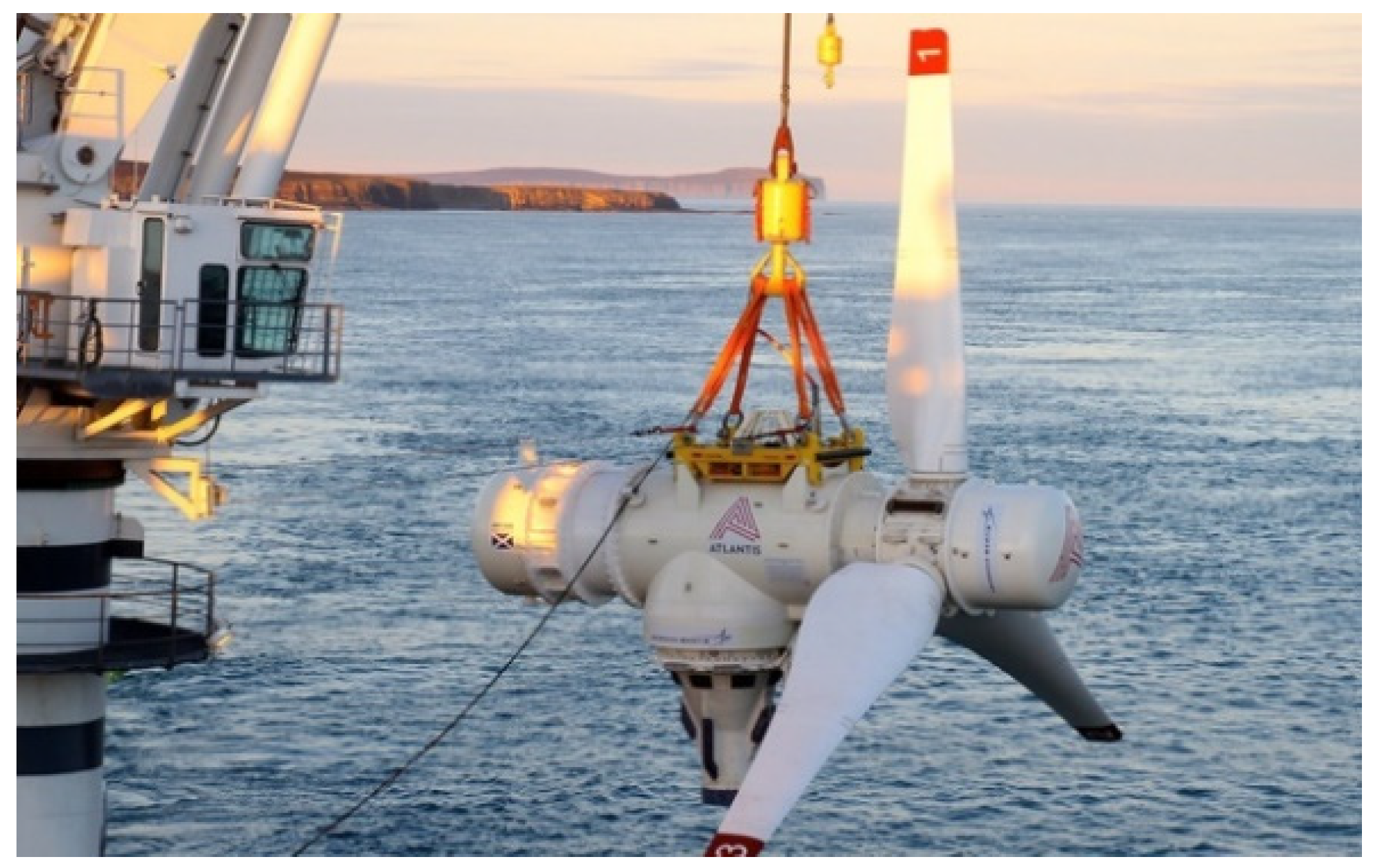Figure 1 shows the example of the AR2000 horizontal tidal turbine (HATT). Vertical axis tidal turbines and other topologies are also used to harness tidal energy but most of the research and development efforts are focused on horizontal axis tidal turbine [5]. Therefore, the AR2000 tidal turbine whose characteristics are described in

Table 1. AR200Horizontal Axis Tidal turbine parameters [7].

Item	Value
Rated Power (kW)	2000
Rotation diameter (m)	20
Height from the seabed (m)	25
Swept area of rotor (m2)	314
Cut-in speed (m/s)	1
Cut-out speed (m/s)	3
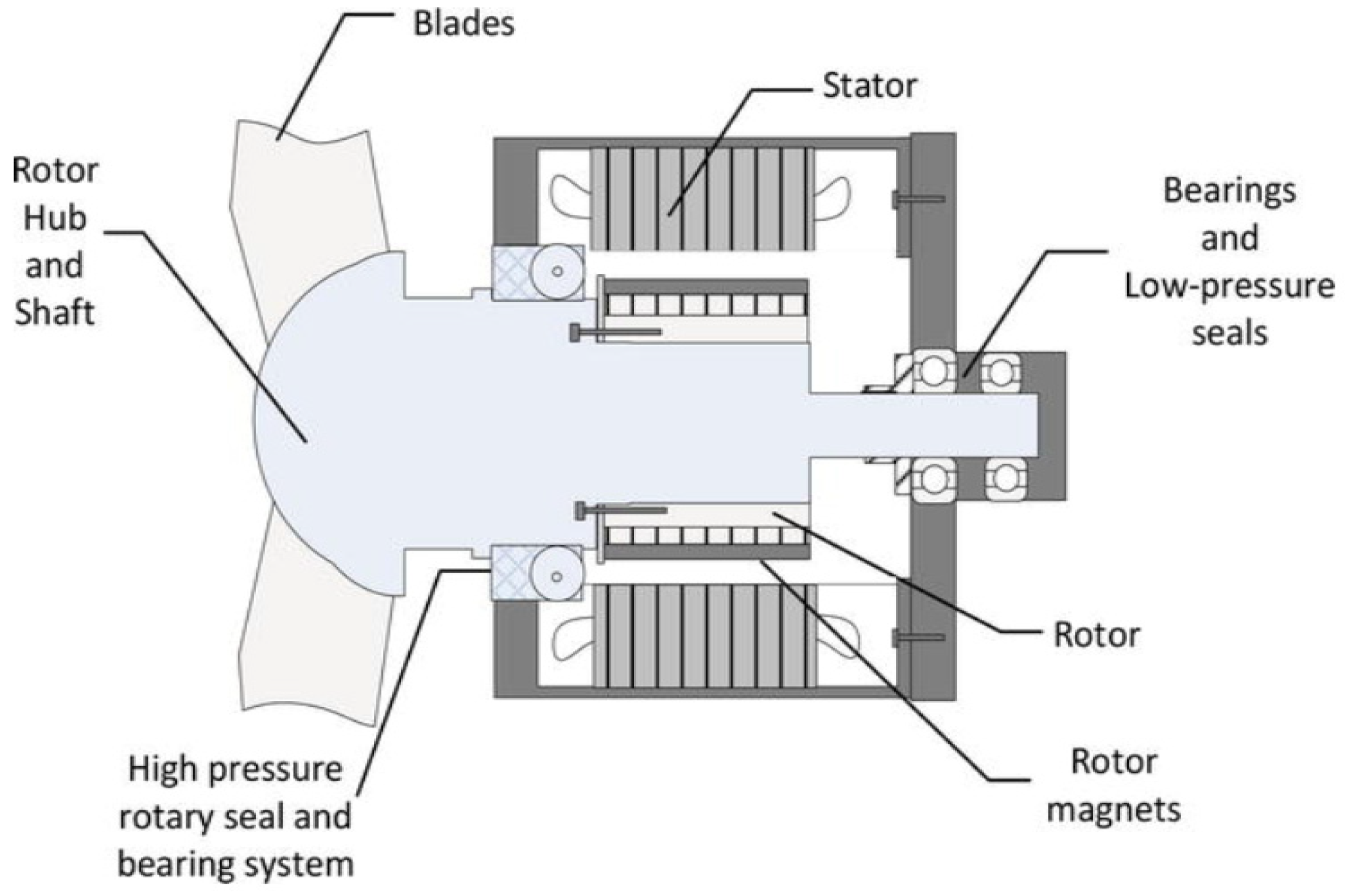
Mass (t)	150

will be used in the present study as support for our design methodology. The submerged electrical machine is considered completely enclosed with an airgap filled with air under pressure in order to help the cooling. Such an architecture is represented in Figure 2.

In the specific case of tidal turbines, the main challenge of the designer is to size the electrical generator considering the working cycle while managing all the constraints, especially the thermal one because the machine never operates in a steady state. It is also of great interest to take into account the control strategy by optimizing the current and voltage parameters according to variable operating points. Whereas conventional solutions prefer synchronous permanent magnet machines [9,10], the use of Electrically Excited Synchronous Generators remains an interesting solution. The removal of magnets from electrical machines is actually increasingly investigated in order to free themselves from their excessive and highly fluctuating cost and the risks of supply disruption in a very tight market [11,12]. If, for wind turbines, the predominant mass criterion naturally involves the use of permanent magnet generators, for tidal turbines placed on the sea bottom, this criterion can be put in second place, and we can focus on energy efficiency instead. In the light of these observations, the EESG becomes an interesting solution. Note also that with EESG, dangerous overcurrents can be avoided in case of a short circuit.

In the field of renewable energies like tidal harvesting energy, the generator is generally designed for the rated power [13,14,15,16]. However, in the light of the intermittence of renewable energy sources, using such a method may lead to oversize the generator particularly if the permanent thermal regime is never reached. All points of the operating cycle must therefore be taken into account to calculate the temperature profile during the working cycle. A cycle often consists of hundreds or even several thousands of operating points. Thus, taking into account all points of the cycle in the optimization process by a genetic algorithm, for example, constitute a real problem in terms of computation time. In order to solve this problem today, the only way consists of replacing all working points by a representative point or, in the best case, to reduce the study by a few points from an analysis of the energy distribution over the cycle [17,18,19,20,21,22]. For example, in [23], the authors reduce the whole cycle to only two points. In [24], which deals with the design of a Direct Drive Permanent Magnet Generator for a Tidal Current Turbine, the objective function, in addition to the material cost, is made of 10 discrete operating points associated to the probability density of each operating point. However, such an approach is approximate because it ignores the temporal variations that is necessary to manage correctly the thermal transient and the control strategy to maximize the efficiency. In addition, because the thermal dynamic analysis was not considered, the maximum temperature elevation calculated is equivalent to the temperature elevation calculated with a continuous rated power.

Therefore, this paper focuses on an approach allowing to solve the complete problem without an excessive increase in calculation time. Developed for the first time in [25] the method was based on a 1D analytical model and applied to the case of a PMSM. It was shown how it is possible to optimize a machine from the torque and speed profiles. However, the thermal transient was not taken into account and the armature reaction was neglected. We propose therefore to complete this approach and apply it for the first time to the case of the EESG. To our knowledge, such an approach has been never made for this machine. In this paper, the objective is to size a generator from the torque and speed profiles supplied by the turbine AR2000 with the variation of the tidal currents that we took at the French coast in the Raz de Sein.

The paper is organized as follows: the analytical model used is developed in Section 2. Section 3 describes the optimization methodology and the way to solve the problem. Section 4 presents the application and the results of the selected optimal machine with its optimal geometry and optimum control parameters. The design of the selected machine is finally validated by a 2D Finite Element Analysis.

2. 1D Analytical Modeling

In this section, analytical modeling of the EESG is proposed with the aim of optimization. The design and the main geometrical parameters are illustrated in Figure 3. This analytical model is commonly used in machine design and optimization [26]. Its accuracy and efficiency have already been demonstrated. In this paper, we will recall the main equations and hypotheses necessary to understand the problem. For more details, the reader can refer to the following references [26,27].

2.1. Electromagnetic Model

The iron core permeability is assumed infinite, and the analytical model of the EESG is limited to the fundamental component. However, a coefficient ${\eta }_t$ will be introduced in the calculation of iron losses to take into account the effects of the harmonic components [28]. The stator is assumed to have radial teeth and slots with the coils connected to form a three-phase winding. Each phase is made of a distributed winding with $N_{es}$ slots/pole/phase. The salient rotor has rectangular slots with a DC current field winding. (see Figure 3a).

The optimization approach is based on the use of the equivalent electrical model of the machine in the dq reference frame (see Figure 4) taking iron losses into account via the resistance ${ℛ}_{\mu }$ [29]. The goal of the proposed model is then to express ${ℛ}_c$, ${ℛ}_{\mu }$, $X_d$, $X_q$, and $e_0$ as functions of the optimization parameters.

2.1.1. Electrical Equations

In this paper, we assume the terms $d{i}_{od}/dt$ and $d{i}_{oq}/dt$ negligible, which can be easily assumed with the low speed variations observed in the tidal energy application. Then, the main equations related to the voltages $v_{od}\left(t\right)$ and $v_{od}\left(t\right)$, and the electromagnetic power $P_{em}\left(t\right)$ are:

$$v_{od}\left(t\right)=X_q\left(t\right)i_{oq}\left(t\right)$$

(1)

$$v_{oq}\left(t\right)=e_0\left(t\right)-X_d\left(t\right)i_{od}\left(t\right)$$

(2)

$$P_{em }\left(t\right)=e_0\left(t\right)i_{oq}\left(t\right)-\left(X_d\left(t\right)-X_q\left(t\right)\right)i_{od}\left(t\right)·i_{oq}\left(t\right)$$

(3)

With the back e.m.f. $e_0,$ proportional to the rotor current $I_f.$ It that can be written in the form:

$$e_0\left(t\right)=k{I}_f\mathsf{\Omega }\left(t\right)$$

(4)

The copper losses, in the stator and the rotor windings, are given by:

$$P_c\left(t\right)={ℛ}_c\left(i_d^2\left(t\right)+i_q^2\left(t\right)\right)+{ℛ}_f{I}_f^2\left(t\right)$$

(5)

And the iron losses:

$$P_{mg}\left(t\right)=\frac{v_{od}^2\left(t\right)+v_{oq}^2\left(t\right)}{R_{\mu }\left(t\right)}$$

(6)

2.1.2. Flux Densities

The fundamental airgap flux density created by the rotor current, obtained from Ampere’s law is:

$$B_f\left(t,\theta \right)=\frac{4}{\pi }\frac{{\mu }_0{n}_f}{e}\sin \left(\frac{p\beta }{2}\right)I_f\left(t\right) \sin \left(p\left(\theta -{\theta }_r\right)\right)$$

(7)

With $\beta$, the electrical arc of the rotor pole and $n_f$ the number of turns per pole at the rotor. Then, the magnitude is:

$$B_{fm}\left(t\right)=\frac{2}{\pi }\frac{{\mu }_0{n}_f}{e}\sin \left(\frac{p\beta }{2}\right)I_f\left(t\right)$$

(8)

The fundamental airgap flux density created by the stator can be expressed since the surfacic perméance $\mathcal{P}$ such as:

$$B_s(\theta ,t)=F_{mm}(\theta ,t)\mathcal{P}\left(\theta ,{\theta }_r\right)$$

(9)

With:

$$F_{mm}\left(\theta ,t\right)=\frac{6}{\pi }{n}_s{I}_s\left(t\right)\cos \left(p\theta -\omega t-\psi \left(t\right)\right)$$

(10)

$$\mathcal{P}\left(\theta ,{\theta }_r\right)={\mathcal{P}}_0+{\mathcal{P}}_{1}cos\left(2p\left(\theta -{\theta }_r\right)\right)$$

(11)

where $F_{mm}$ is the first harmonic of the stator magnetomotive force (MMF) created by the three phases and $\mathcal{P}$ the surfacic permeance limited to the fundamental. According to the distribution of $\mathcal{P}$ represented in Figure 3b, the average value ${\mathcal{P}}_0$ and the magnitude of the fundamental ${\mathcal{P}}_1$ are:

$${\mathcal{P}}_0=\frac{{\mu }_0}{R_{sS}-R_{wr}}+\frac{p\beta }{\pi }\left(\frac{{\mu }_0}{e}-\frac{{\mu }_0}{R_{sS}-R_{wr}}\right)$$

(12)

$${\mathcal{P}}_1=\frac{2}{\pi }\left(\frac{{\mu }_0}{e}-\frac{{\mu }_0}{R_{ss}-R_{wr}}\right)sin\left(p\beta \right)$$

(13)

Since ${\theta }_r=\mathsf{\Omega }t=\omega /p$ and substituting Equations (10)–(13), into the Equation (9), it is possible to demonstrate that:

$$B_s\left({\theta }_s,t\right)=\frac{6}{\pi }{n}_s{I}_s\left(t\right)\left[\left({\mathcal{P}}_0+\frac{{\mathcal{P}}_1}{2}\right)sin\left(\psi \left(t\right)\right)cos(\omega t-p\theta )+\left({\mathcal{P}}_0-\frac{{\mathcal{P}}_1}{2}\right)cos\left(\psi \left(t\right)\right)sin(\omega t-p\theta )\right]$$

(14)

With:

$$i_d\left(t\right)=I_s\left(t\right)\sin \left(\psi \left(t\right)\right)$$

(15)

$$i_q\left(t\right)=I_s\left(t\right)\cos \left(\psi \left(t\right)\right)$$

(16)

The magnitude of the flux density in the airgap $B_{sm}$ can be deduced and expressed as:

$$B_{sm}\left(t\right)=\frac{6}{\pi }\sqrt{{\left(\left({\mathcal{P}}_0+\frac{{\mathcal{P}}_1}{2}\right)n_s{i}_d\left(t\right)\right)}^2+{\left(\left({\mathcal{P}}_0-\frac{{\mathcal{P}}_1}{2}\right)n_s{i}_q\left(t\right)\right)}^2}$$

(17)

Then, the resulting flux density in the airgap $B_{rm}$ is obtained since:

$$B_{rm}^2\left(t\right)=B_{fm}{\left(t\right)}^2+B_{sm}{\left(t\right)}^2+2B_{fm}\left(t\right)B_{sm}\left(t\right)\sin \left(\psi \left(t\right)\right)$$

(18)

Thanks to the Gauss’s law, it is possible to express the magnitude of the flux densities in the stator tooth ($B_{stm}$), stator yoke ($B_{sym}$), rotor tooth ($B_{rtm}$), and rotor yoke ($B_{rym}$). It gives:

$$B_{stm}\left(t\right)=\frac{1}{k_{ts}}{B}_{rm}\left(t\right)$$

(19)

$$B_{sym}\left(t\right)=\frac{R_{ss}}{p\left(R-R_{ws}\right)}{B}_{rm}\left(t\right)$$

(20)

$$B_{rtm}\left(t\right)=\frac{1}{k_{tr}}{B}_{rm}\left(t\right)$$

(21)

$$B_{rym}\left(t\right)=\frac{R_{ss}}{p\left(R_{wr}-R_0\right)}{B}_{rm}\left(t\right)$$

(22)

2.1.3. Back E.M.F.

Since the Faraday’s law and Equation (8), the constant $k$ in Equation (4) is:

$$k=\frac{8\sqrt{6}}{\pi }\frac{{\mu }_0{k}_w{n}_s{n}_f{\tau }_{LR}R{R}_{ss}}{e}\sin \left(\frac{p\beta }{2}\right)$$

(23)

2.1.4. Resistances and Inductances

According to [27], it is possible to demonstrate that the stator electrical resistance can be written:

$${ℛ}_c=\frac{48}{\pi } \left(\frac{k_{Ls}}{{\sigma }_c{k}_{fs}\left(1-k_{ts}\right)}\right)n_s^2{\tau }_{LR}R\frac{p^2}{R_{ws}^2-R_{ss}^2}$$

(24)

And the rotor electrical resistance:

$${ℛ}_f=\frac{16}{\pi }\left(\frac{k_{Lr}}{{\sigma }_c{k}_{f\mathrm{r}}\left(1-k_{tr}\right)}\right)n_f^2{\tau }_{LR}R\frac{p^2}{R_{sr}^2-R_{wr}^2}$$

(25)

where $k_{Ls-r}$, $k_{fs-r}$ and $k_{ts-r}$ are respectively, a coefficient that corrects the active length due to end windings (stator-rotor), the slot fill factor (stator-rotor), and the tooth opening to the slot pitch ratio (stator-rotor).

Neglecting the iron losses on the rotor, the iron losses (Eddy currents + hysteresis) can be also written as a function of $B_{rm}$ as described in [25] such as:

$$P_{mg}\left(t\right)=P_{ymg}\left(t\right)+P_{tmg}\left(t\right)=\pi k_{ad}{\eta }_t^2\left(k_{ec}{p}^2{\mathsf{\Omega }}^2\left(t\right)+k_{h}p\mathsf{\Omega }\left(t\right)\right)\left({\gamma }_y+{\gamma }_t\right)B_{rm}^2\left(t\right)$$

(26)

With ${\gamma }_t$ and ${\gamma }_y$, functions depending on geometric parameters and speed [25]:

$$\begin{gathered} {\gamma }_y=\frac{\left(R+R_{ws}\right)R^3}{\left(R-R_{ws}\right)p}{\tau }_{LR} \\ {\gamma }_t=\frac{1}{k_{ts}}\frac{R\left(R_{ws}^2-R_{ss}^2\right)R_s}{R_{ws}}{\tau }_{LR} \end{gathered}$$

(27)

Thus, from Equations (6), (26), and (27) it is possible to write:

$${ℛ}_{\mu }\left(t\right)=\frac{24}{\pi }{n}_s^2{\tau }_{LR}R\frac{p\mathsf{\Omega }\left(t\right)}{k_{ad}{\eta }_t^2\left(k_{ec}p\mathsf{\Omega }\left(t\right)+k_h\right)}\frac{1}{\frac{1}{k_{ts}}\frac{R_{ws}^2-R_{ss}^2}{R_{ss}{R}_{ws}}+\frac{R^2-R_{ws}^2}{p^2{\left(R-R_{ws}\right)}^2}}$$

(28)

The d-q inductances can be calculated since Equations (12) and (13). It gives:

$${\mathcal{L}}_d=\frac{24}{\pi }\left({\mathcal{P}}_0+\frac{{\mathcal{P}}_1}{2}\right)n_s^2{R}_{ss}{\tau }_{LR}Rx$$

(29)

$${\mathcal{L}}_q=\frac{24}{\pi }\left({\mathcal{P}}_0-\frac{{\mathcal{P}}_1}{2}\right)n_s^2{R}_{sS}{\tau }_{LR}R$$

(30)

2.2. Thermal Model

During operation, the hottest point in the machine must remain smaller than the maximum permissible temperature in the windings during the working cycle. The dynamic behavior of the temperature in the windings must therefore be calculated. In this case, the use of a lumped parameter thermal model [30] is adapted and has shown its efficiency for EESG [31,32]. Figure 5 represents the equivalent circuit used to calculate the temperature evolution in the rotor and stator windings. The following assumptions are made:

• no heat flux in the axial direction in the stator and rotor iron because of the lamination,
• the frame is considered to be a perfect thermal conductor,
• no axial heat flux in the airgap,
• conductors in the slot are uniformly distributed, and
• end windings are considered to be cylindrical and homogenous.

For heat conduction, the thermal resistances as well as the thermal capacities are calculated from the geometry and the thermal properties of the materials. The thermal conductivities considered in this paper are given in

Table 2. Materials thermal conductivities.

Material	$\mathbf{Thermal}\mathbf{Conductivity}\mathit{\lambda }$
Iron	25
Slots (average thermal conductivity of an equivalent homogeneous material with copper and insulation)	5
air	0.025

. For a piece of the cylinder (see Figure 5a), the expressions of the thermal resistances and capacity are [27,33]:

$$R_{thx1}=\frac{1}{2{\lambda }_{mat}{\beta }_{mat}L}\left(\frac{2{\left(\frac{R_{ext}}{R_{int}}\right)}^{2}ln\left(\frac{R_{ext}}{R_{int}}\right)}{{\left(\frac{R_{ext}}{R_{int}}\right)}^2-1}-1\right)$$

(31)

$$R_{thx2}=\frac{1}{2{\lambda }_{mat}{\beta }_{mat}L}\left(1-\frac{2ln\left(\frac{R_{ext}}{R_{int}}\right)}{{\left(\frac{R_{ext}}{R_{int}}\right)}^2-1}\right)$$

(32)

$$C_x=C_{px}\frac{1}{2\pi }{\rho }_{mat}{\beta }_{mat}\left(R_{ext}^2-R_{int}^2\right)L$$

(33)

The thermal resistance in the axial direction from the slots to the end windings ($R_{thsw3}$ and $R_{thrw3}$) is calculated by:

$$R_{th x3}=\frac{L}{{\lambda }_{mat}{\beta }_{mat}\left(R_{ext}^2-R_{int}^2\right)}$$

(34)

For convective heat transfer, the thermal resistance at corresponding interfaces $R_{thcvx}$ ($R_{thcv ext}$, $R_{thcv a}$ and $R_{thcv ew}$) with area $A_x$ and convective heat coefficient $h_x$ is calculated using the following expression:

$$R_{thcvx}=\frac{1}{h_x{A}_x}$$

(35)

In the considered case, according to [34], we assume that heat is considered to be extracted at an external radius $R$ by a forced convection with $h_{ext}=280$ W/m² K and the convective heat coefficient in end-windings is $h_{ew}=15$ W/m² K.

Considering the heat transfer in the airgap, without axial transfer, the convective heat coefficient is expressed [33] as:

$$h_a=\frac{Nu{\lambda }_{air}}{2e}$$

(36)

Considering the Nusselt number, the choice of the following calculation has been conducted. At each speed, according to [33], $Nu$ is calculated from the modified Taylor number $T{a}_m$ evaluated by the following equations:

$$T{a}_m=\frac{T_a}{F_g}$$

(37)

With:

$$Ta=\frac{{\rho }_{air}^2{\mathsf{\Omega }}^2{R}_m{e}^3}{{\mu }_{air}^2}$$

(38)

$$F_g=\frac{{\pi }^4}{P}\frac{1}{1697{\left(1-\frac{e}{2R_m}\right)}^2}$$

(39)

$$P=0.0571\left(1-0.625\frac{2e}{2R_m-e}\right)+\frac{0.00056}{1-0.625\frac{2e}{2R_m-e}}$$

(40)

where: $R_m$ is the radius in the middle of the airgap, $\mathsf{\Omega }$ is the rotational speed, ${\rho }_{air}$ is the mass density of air, and ${\mu }_{air}$ is the dynamic viscosity of air.

The values of the Nusselt number we have chosen, used by most authors [27,33,34,35,36], are:

$$\{\begin{array}{ll}Nu=2\hfill & \left(0<T{a}_m<1700\right)\hfill \\ Nu=0.128 T{a}_m^{0.367}\hfill & \left(1700<T{a}_m<{10}^4\right)\hfill \\ Nu=0.409 T{a}_m^{0.241}\hfill & \left(0<T{a}_m<{10}^7\right)\hfill \end{array}$$

(41)

Since the equivalent circuit and the knowledge of thermal resistances, the calculation of the temperature at each node can be solved. The general transient equation for the thermal network is given by:

$$C_i\frac{d{\theta }_i\left(t\right)}{dt}=P_i\left(t\right)-{\displaystyle \sum }_{j=1}^n\frac{{\theta }_i\left(t\right)-{\theta }_j\left(t\right)}{{ℛ}_{ij}}$$

(42)

where ${\theta }_i$, ${\theta }_j$ and ${ℛ}_{ij}$ are respectively the temperature at node $i$, the temperature at node $j$ and the thermal resistance between nodes $i$ and $j$.

3. Optimization Problem

3.1. Problem Statement

We propose to optimize at the same time the design and the control of the generator with the following two objectives: the minimization of the electrical energy losses during the working cycle and the minimization of the mass. In addition to the thermal and saturation constraints, we introduce a voltage limit $V_{limit}$ imposed by the power electronics converter and a minimum thickness for the stator and rotor yokes ($W_{sy}$ and $W_{ry})$. The height of the rotor pole shoe $W_{rps}$ is assumed to be 10% of the pole pitch and the rotor pole opening factor β is fixed to 7/8 [26]. Thus, the problem is:

Objectives:

$$\begin{gathered} \underset{x}{\mathit{min}}\left(W_{losses}=\underset{cycle}{\overset{}{{\displaystyle \int }}}\left(P_{tot}\left(t\right)\right)dt\right) \\ \underset{x}{\mathit{min}}\left(Mass=M_c+M_i\right) \end{gathered}$$

(43)

Constraints:

$$\begin{gathered} max\left\{{\theta }_{ws}\left(t\right);{\theta }_{wr}\left(t\right);{\theta }_{wer}\left(t\right);{\theta }_{wer}\left(t\right)\right\}\le {\theta }_{max}=160°\mathrm{C} \\ max\left\{B_{stm}\left(t\right);B_{sym}\left(t\right);B_{rtm}\left(t\right);B_{rym}\left(t\right)\right\}\le B_{sat}=1.5\mathrm{T} \\ max\left\{V_{max}\left(t\right)=\sqrt{\frac{2}{3}}\sqrt{V_d^2\left(\mathrm{t}\right)+V_q^2\left(t\right)}\right\}\le V_{limit}=2500\mathrm{V} \\ min\left\{W_{sy};W_{ry}\right\}\ge W_{min}=10\mathrm{mm} \end{gathered}$$

(44)

With:

$$x={\left(p,R,R_{ws},R_{ss},R_{sr},R_{wr},{\tau }_{LR},n_s,i_d\left(t\right),i_q\left(t\right),I_f\left(t\right)\right)}^T$$

(45)

3.2. Optimization Methodology

It is recalled here that the goal is to size a machine and its control strategy from a working cycle made of several thousand points. The proposed solution must fulfill all the constraints for all operating points (particularly the temperature evolution that must be calculated since the heat equation in the transient regime) while keeping a reduced computation time. To reduce the computation time, the other authors limit the sizing to either the maximum power (which leads to an oversizing), or to a reduced number of points in the cycle in order to avoid an oversizing. However, in both cases, neither the control strategy nor the control of the thermal transient is taken into account in the optimization process. The principle of the proposed optimization is based on the predetermination of the control parameters analytically according to the torque and speed profiles. For each working point, these parameters ($i_{od}\left(t\right),i_{oq}\left(t\right)$ and $I_f\left(t\right)$) are expressed analytically as functions of other optimization variables. This step is the key to reduce the calculation time. In a second step, the energy lost per working cycle (the first objective function) is expressed as a function of the geometric variables which are time-independent optimization variables. This allows the optimization algorithm to optimize scalar variables only, which allows it to have a reduced calculation time. (Figure 6).

3.2.1. Expressions of Optimal Control Parameters

The goal for this first step is therefore to express the losses as a function of the control parameters. From (1)–(6), it is possible to express the copper losses as follows:

$$\begin{array}{l}{P}_c\left(t\right)=i_{od}^2\left(t\right)\left[\begin{array}{c}{ℛ}_c \left(1+\frac{X_q{\left(t\right)}^2}{R_{\mu }^2\left(t\right)}\right)+\dots \\ \dots +{ℛ}_f{\left(\frac{X_d\left(t\right)-X_q\left(t\right)}{k\omega \left(t\right)}\right)}^2 \end{array}\right]+i_{oq}^2\left(t\right)\left[{ℛ}_c\left(1+\frac{X_q{\left(t\right)}^2}{R_{\mu }^2\left(t\right)}\right)\right]+2{ℛ}_c\frac{P_{em}\left(t\right)}{R_{\mu }\left(t\right)}+\dots \\ \dots +\frac{1}{i_{oq}^2\left(t\right)}\left[{ℛ}_c{\left(\frac{P_{em}\left(t\right)}{R_{\mu }\left(t\right)}\right)}^2+{ℛ}_f{\left(\frac{P_{em}\left(t\right)}{k\omega \left(t\right)}\right)}^2\right]+\frac{i_{od}\left(t\right)}{i_{oq}\left(t\right)}\left[\begin{array}{c}2{ℛ}_c{X}_q\left(t\right) \frac{P_{em}\left(t\right)}{R_{\mu }^2\left(t\right)}+\dots \\ \dots -2{ℛ}_f\frac{P_{em}\left(t\right)}{R_{\mu }^2\left(t\right)}\left(X_d\left(t\right)-X_q\left(t\right)\right)\end{array}\right]\end{array}$$

(46)

And the iron losses as:

$$P_{mg}\left(t\right)=i_{od}^2\left(t\right)\left(\frac{X_q{\left(t\right)}^2}{R_{\mu }\left(t\right)}\right)+i_{oq}^2\left(t\right)\left(\frac{X_q{\left(t\right)}^2}{R_{\mu }\left(t\right)}\right)+\frac{i_{od}\left(t\right)}{i_{oq}\left(t\right)}\left(2\frac{P_{em}\left(t\right)}{R_{\mu }\left(t\right)}\right)+\frac{1}{i_{oq}^2\left(t\right)}\left(\frac{P_{em}^2\left(t\right)}{R_{\mu }\left(t\right)}\right)$$

(47)

Then the total electrical losses can be written in the form:

$$P_{tot}\left(t\right)=A\left(t\right)i_{od}^2\left(t\right)+B\left(t\right)i_{oq}^2\left(t\right)+C\left(t\right)\frac{1}{i_{oq}^2\left(t\right)}+D\left(t\right)\frac{i_{od}\left(t\right)}{i_{oq}\left(t\right)}+E\left(t\right)$$

(48)

where the terms $A\left(t\right)$, $B\left(t\right)$, $C\left(t\right)$, $D\left(t\right)$ and $E\left(t\right)$ depend on the power profile and the optimization variables ($p,R,R_{ws},R_{ss},R_{sr},R_{wr},{\tau }_{LR},n_s$):

$$A\left(t\right)={ℛ}_c\left(1+\frac{X_q{\left(t\right)}^2}{R_{\mu }^2\left(t\right)}\right)+{ℛ}_f{\left(\frac{X_d\left(t\right)-X_q\left(t\right)}{k\omega \left(t\right)}\right)}^2+\left(\frac{X_q{\left(t\right)}^2}{R_{\mu }\left(t\right)}\right)$$

(49)

$$B\left(t\right)={ℛ}_c\left(1+\frac{X_q{\left(t\right)}^2}{R_{\mu }^2\left(t\right)}\right)+\left(\frac{X_q{\left(t\right)}^2}{R_{\mu }\left(t\right)}\right)$$

(50)

$$C\left(t\right)={ℛ}_c{\left(\frac{P_{em}\left(t\right)}{R_{\mu }\left(t\right)}\right)}^2+{ℛ}_f{\left(\frac{P_{em}\left(t\right)}{k\omega \left(t\right)}\right)}^2+\left(2\frac{P_{em}\left(t\right)}{R_{\mu }\left(t\right)}\right)$$

(51)

$$D\left(t\right)=2{ℛ}_c{X}_q\left(t\right)\frac{P_{em}\left(t\right)}{R_{\mu }^2\left(t\right)}-2{ℛ}_f\frac{P_{em}\left(t\right)}{R_{\mu }^2\left(t\right)}\left(X_d\left(t\right)-X_q\left(t\right)\right)+2\frac{P_{em}\left(t\right)}{R_{\mu }\left(t\right)}$$

(52)

$$E\left(t\right)=2{ℛ}_c\frac{P_{em}\left(t\right)}{R_{\mu }\left(t\right)}$$

(53)

From Equation (48), the optimal d-q currents expressions minimizing the total losses, at any time, can be obtained by solving the following system:

$$\{\begin{array}{c}\frac{\partial P_{tot}}{\partial i_{od}}=2A{i}_{od}+\frac{D}{i_{oq}}=0\\ \frac{\partial P_{tot}}{\partial i_{oq}}=2B{i}_{oq}-\frac{2C}{i_{oq}^3}-D\frac{i_{od}}{i_{oq}^2}=0\end{array}$$

(54)

Which leads to:

$$i_{odopt}\left(t\right)=-\frac{D\left(t\right)}{2A\left(t\right)}{\left(\frac{4A\left(t\right)B\left(t\right)}{4A\left(t\right)C\left(t\right)-D\left(t\right)}\right)}^{1/4}$$

(55)

$$i_{oqopt}\left(t\right)=-{\left(\frac{4A\left(t\right)C\left(t\right)-D\left(t\right)}{4A\left(t\right)B\left(t\right)}\right)}^{1/4}$$

(56)

Since Equations (55) and (56) and Equations (3) and (4), we obtain the expression of the optimal DC rotor current:

$$I_{fopt}\left(t\right)=\frac{P_{em}\left(t\right)}{k\omega \left(t\right)}{\left(\frac{4A\left(t\right)B\left(t\right)}{4A\left(t\right)C\left(t\right)-D\left(t\right)}\right)}^{1/4}+\left(\frac{X_d\left(t\right)-X_q\left(t\right)}{k\omega \left(t\right)}\right)\frac{D\left(t\right)}{2A\left(t\right)}{\left(\frac{4A\left(t\right)B\left(t\right)}{4A\left(t\right)C\left(t\right)-D\left(t\right)}\right)}^{1/4}$$

(57)

3.2.2. Expression of the First Objective Function

Finally, introducing Equations (55) and (56) in Equation (48), the expression of the total losses is:

$$P_{tot}\left(t\right)={\left(\frac{4A\left(t\right)B\left(t\right)}{4A\left(t\right)C\left(t\right)-D\left(t\right)}\right)}^{1/2}\left(\frac{D^2\left(t\right)}{4A\left(t\right)}+C\left(t\right)+B\left(t\right)-\frac{D^2\left(t\right)}{4A\left(t\right)}+E\left(t\right)\right)$$

(58)

Then, during the working cycle, total energy lost is obtained by integrating Equation (58):

$$W_{losses}=\underset{T_{cyle}}{\overset{}{{\displaystyle \int }}}{\left(\frac{4A\left(t\right)B\left(t\right)}{4A\left(t\right)C\left(t\right)-D\left(t\right)}\right)}^{1/2}\left(\frac{D^2\left(t\right)}{4A\left(t\right)}+C\left(t\right)+B\left(t\right)-\frac{D^2\left(t\right)}{4A\left(t\right)}+E\left(t\right)\right)dt$$

(59)

where the time-dependent variables have been removed. The remaining optimization variables are the geometrical variables only.

3.2.3. Expression of the Second Objective Function

Only the mass of the active parts will be considered here. $M_c$, $M_i$ and are respectively the mass of the copper and the mass of the iron. They are calculated as below:

$$\begin{gathered} M_c=\pi {\tau }_{LR}\left(R_{ws}^2-R_{ss}^2\right)k_{fs}R{\rho }_c+\pi {\tau }_{LR}\left(R_{sr}^2-R_{ws}^2\right)k_{fr}R{\rho }_c \\ {M}_i=\pi {\tau }_{LR}\left(\left(R_{ws}^2-R_{ss}^2\right)k_{ts}+\left(1-R_{ws}^2\right)\right)R{\rho }_{Fe}+\pi {\tau }_{LR}\left(\left(R_{sr}^2-R_{wr}^2\right)k_{tr}+\left(R_{wr}^2-R_o^2\right)\right)R{\rho }_{Fe} \end{gathered}$$

(60)

To minimize the two objective functions, the NSGA II [37] optimization algorithm is used here. Figure 6 represents, in a flowchart, the principle of design optimization.

4. Application

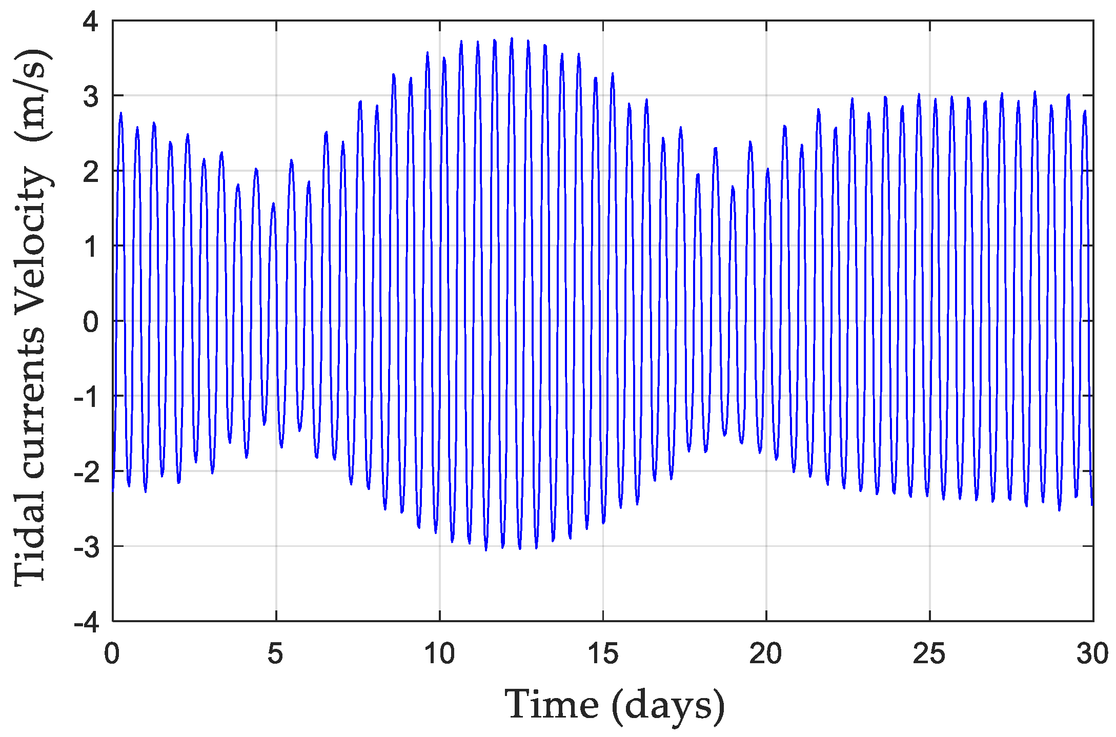
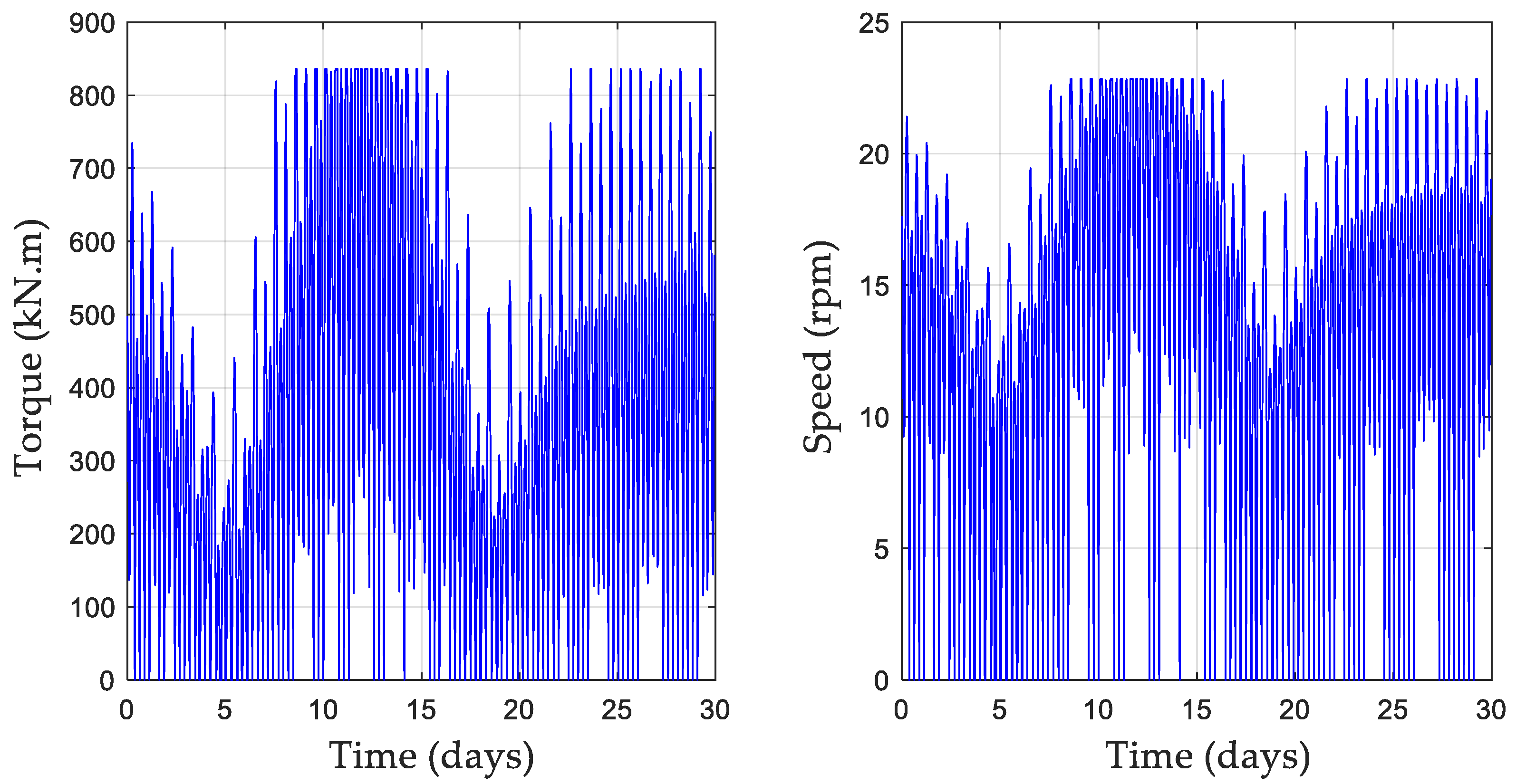
In this section, we present the result of the design optimization based on the method presented in Section 3 and applied to size a 2 MW generator. We have chosen the site at the French coast, in the Raz de Sein, for its high tidal currents velocity. Figure 7 shows the tidal speed profile for the month of highest production (September) made of 720 points (one point per hour) [38]. From these data and the AR200 tidal turbine specifications, the torque and the speed profiles of the generator can be obtained [39] (see Figure 8). The values of the main constant parameters used in this optimization are presented in the Appendix A.

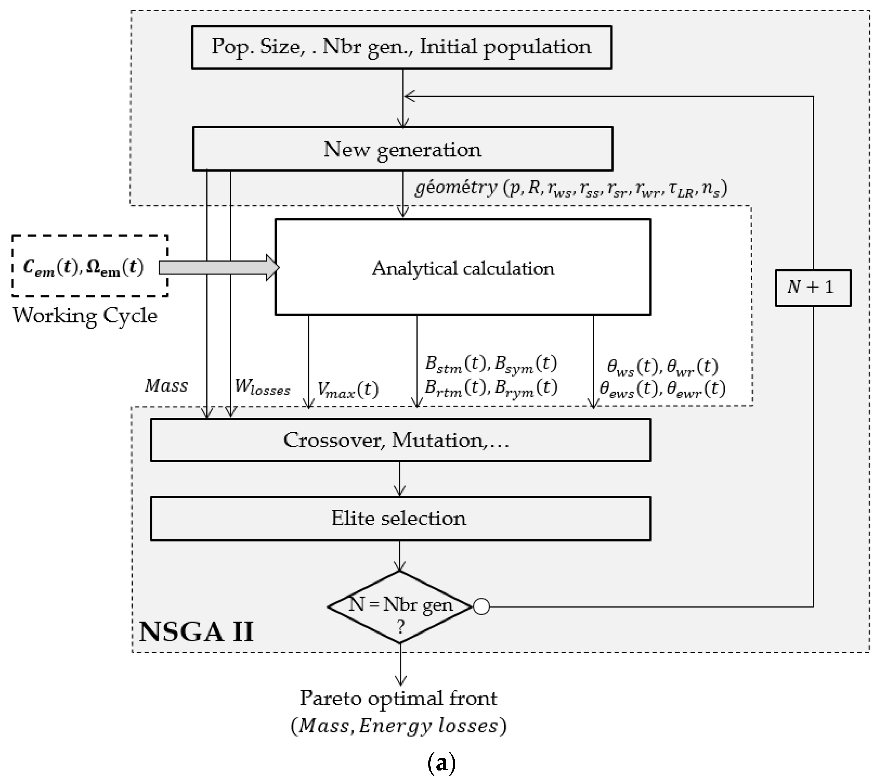
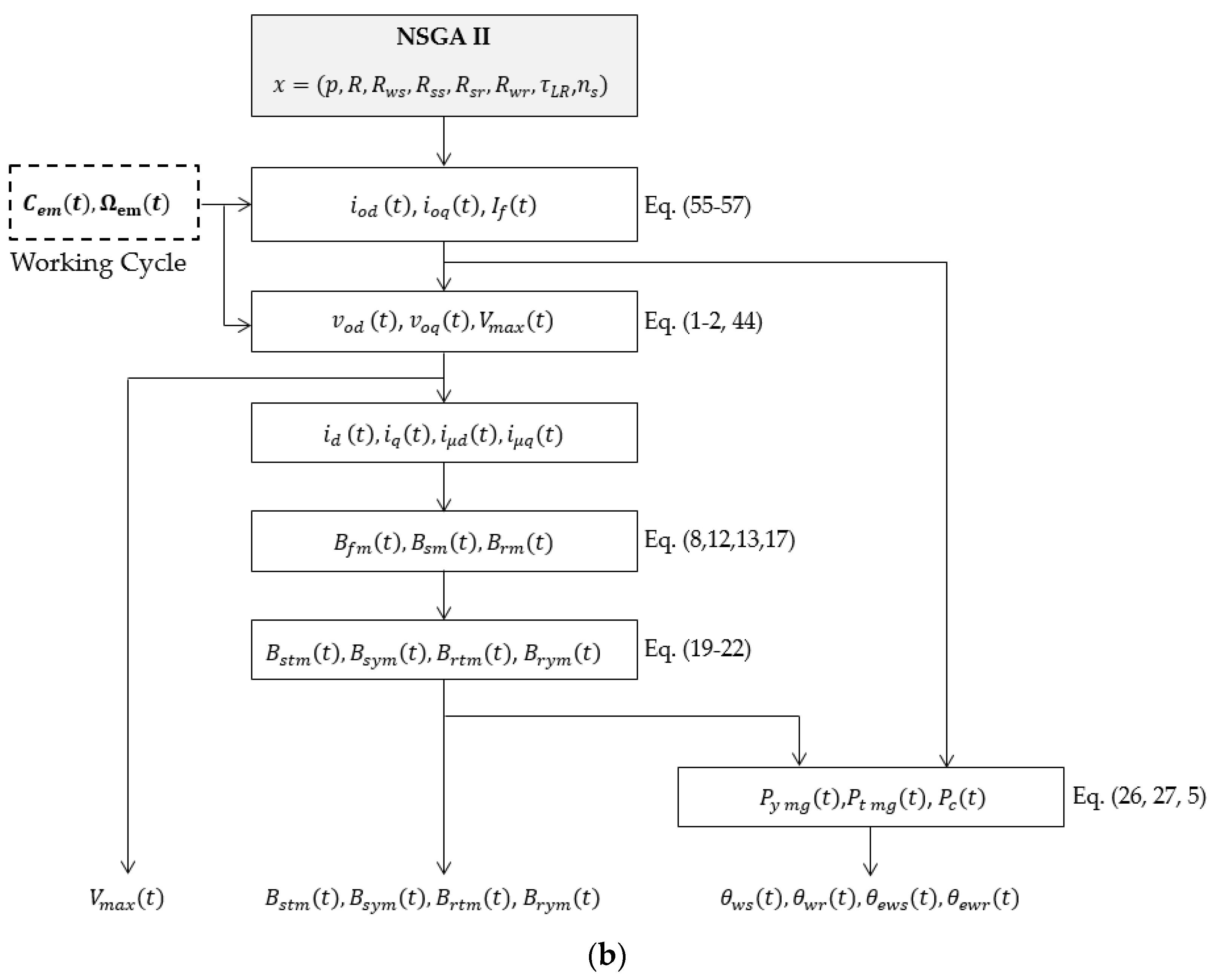
4.1. Optimization Results

The NSGA II has been used with a number of generations and a population size respectively chosen from 2000 to 300. The result is obtained with an acceptable computation time (less than 30 min).

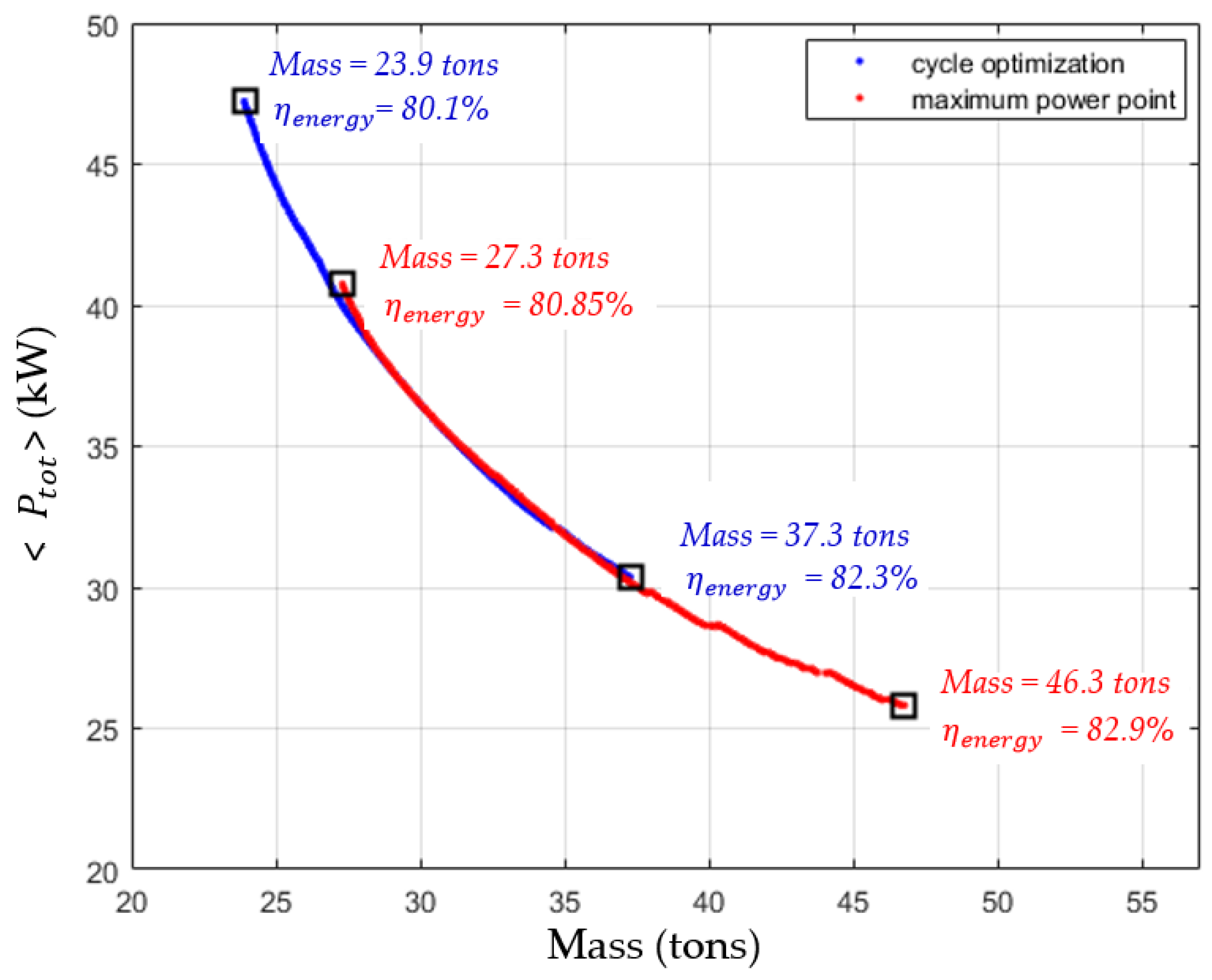
Figure 9 gives the Pareto optimal front obtained. To compare this result with conventional sizing and show the interest of the proposed method, the result of an optimization considering the maximum power point is given (red curve). It can be seen that the optimization at the nominal operating point for this application leads to oversize the generator. For the lightest machines, the difference in mass is greater than 18%. Conversely, the best energy efficiency is obtained for a design at the nominal operating point, but the difference is not significant (less than 2%).

The choice of the optimal geometry is the result of a compromise between mass and efficiency. Such a choice would be the result of a study comparing the manufacturing cost (related to the mass) to the production gains over the life of the machine. Such a study, made possible by the presented method, however, falls outside the scope of the paper and will be developed in a future publication. We will therefore present the result for the lightest optimal machine.

Then, the optimal geometry and the main characteristics of the selected generator are summarized in

Table 3. Optimal generator parameters.

Generator Parameter	Value
$p$	69
$R$	3 m
$n_s$	1
$L$$({\tau }_{LR})$	0.91 m (0.30)
$R_{ws}/R$	0.992
$R_{ss}/R$	0.966
$R_{sr}/R$	0.960
$R_{wr}/R$	0.940
$W_{sy}$	20 mm
$W_{ry}$	20 mm
$e$	6.8 mm
$B_{stm}$	1.5 T
$B_{sym}$	1.49 T
$B_{rtm}$	1.5 T
$B_{rym}$	1.5 T
Total active material weight	23.9 tons
Iron weight	18.15 tons
Copper weight	5.75 tons
Average losses	47 kW
Average copper losses	42 kW
Average iron losses	5 kW
$\mathrm{Nominal}\mathrm{voltage}{V}_s$	1154 V
$\mathrm{Nominal}\mathrm{current}{I}_s$	1323 A
$\mathrm{Self}\mathrm{inductances}{ℒ}_d/{ℒ}_q$	3.6 mH/2.7 mH
$\mathrm{Maximal}\mathrm{stator}\mathrm{current}\mathrm{density}{J}_s$	3.20 A/mm2
$\mathrm{Maximal}\mathrm{rotor}\mathrm{current}\mathrm{density}{J}_r$	2.50 A/mm2
$\mathrm{Nominal}\cos \phi$	0.861

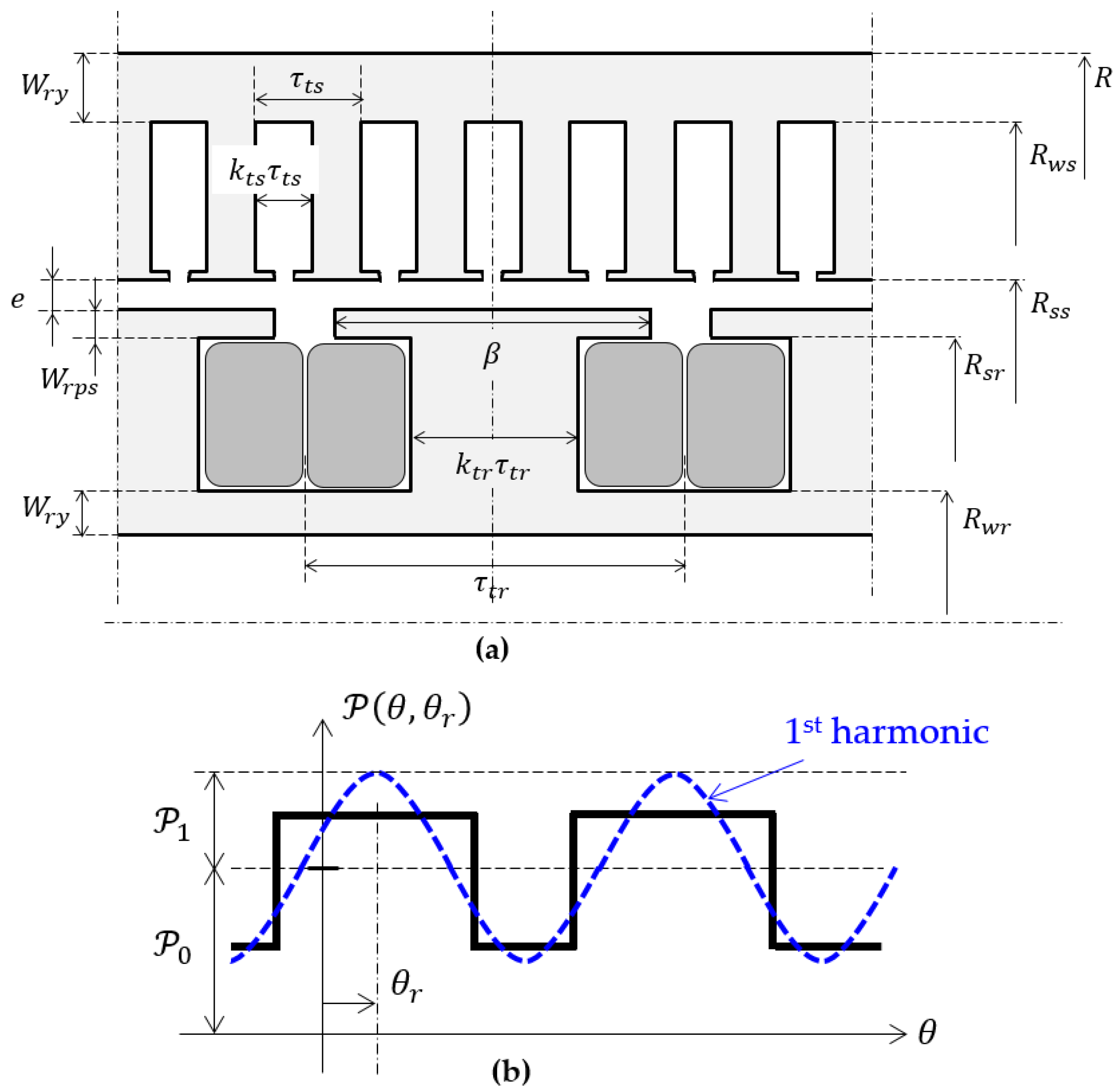
. For this optimization, the saturation and manufacturing constraints (minimum thickness of the yokes) are reached. From the optimal variables ($p,R,R_{ws},R_{ss},R_{sr},R_{wr},{\tau }_{LR}$,$n_s$) found with the NSGA II, which are given in Table 3, the optimal magnetomotive forces $n_s{i}_{od opt}\left(t\right)$, $n_s{i}_{oq opt}\left(t\right)$ and $n_f{I}_{f opt}\left(t\right)$ are calculated afterwards with Equations (49)–(57) such as represented in Figure 6b with $x=x_{opt}$. 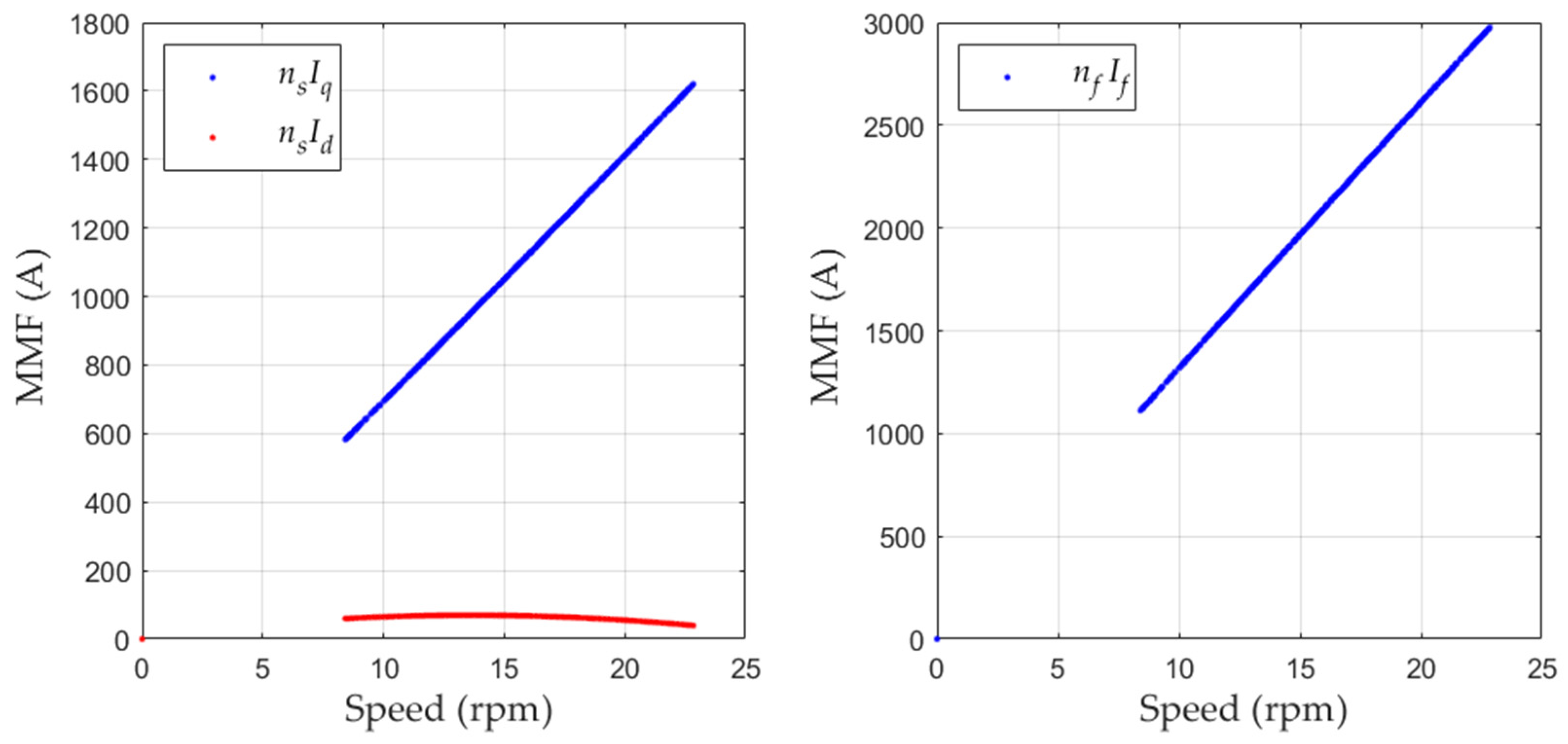In Figure 10, the optimal magnetomotive forces (related to d-q axis stator currents and rotor current) are represented as a function of the mechanical speed. We can observe that the flux weakening is obtained on both the excitation current and the d-axis stator current. However, we can see that the flux weakening is mainly obtained by the rotor winding. In this case, the low value of the $i_d$ component would make it possible to consider a control at $i_d=0$, which would simplify the control of the generator.

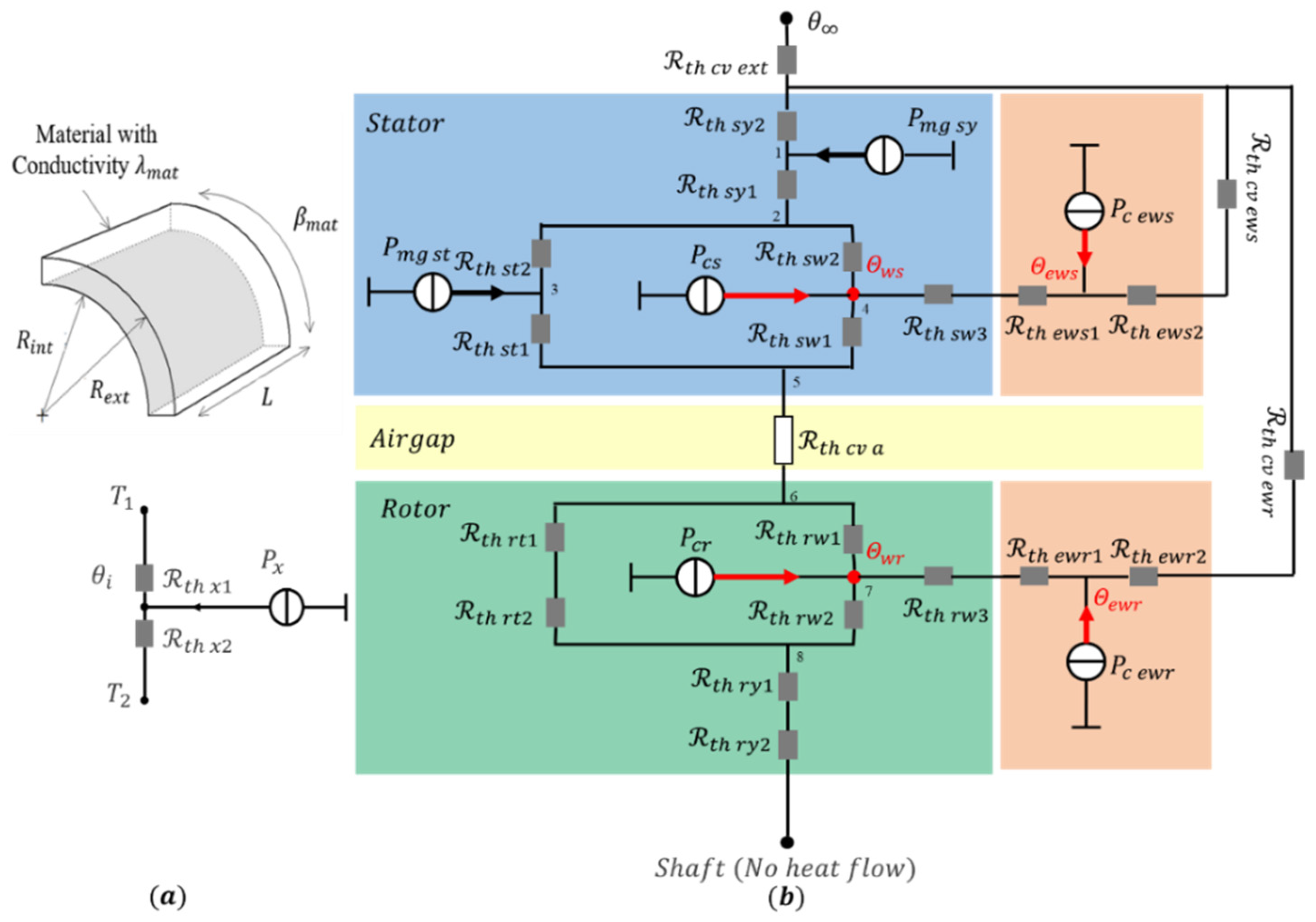
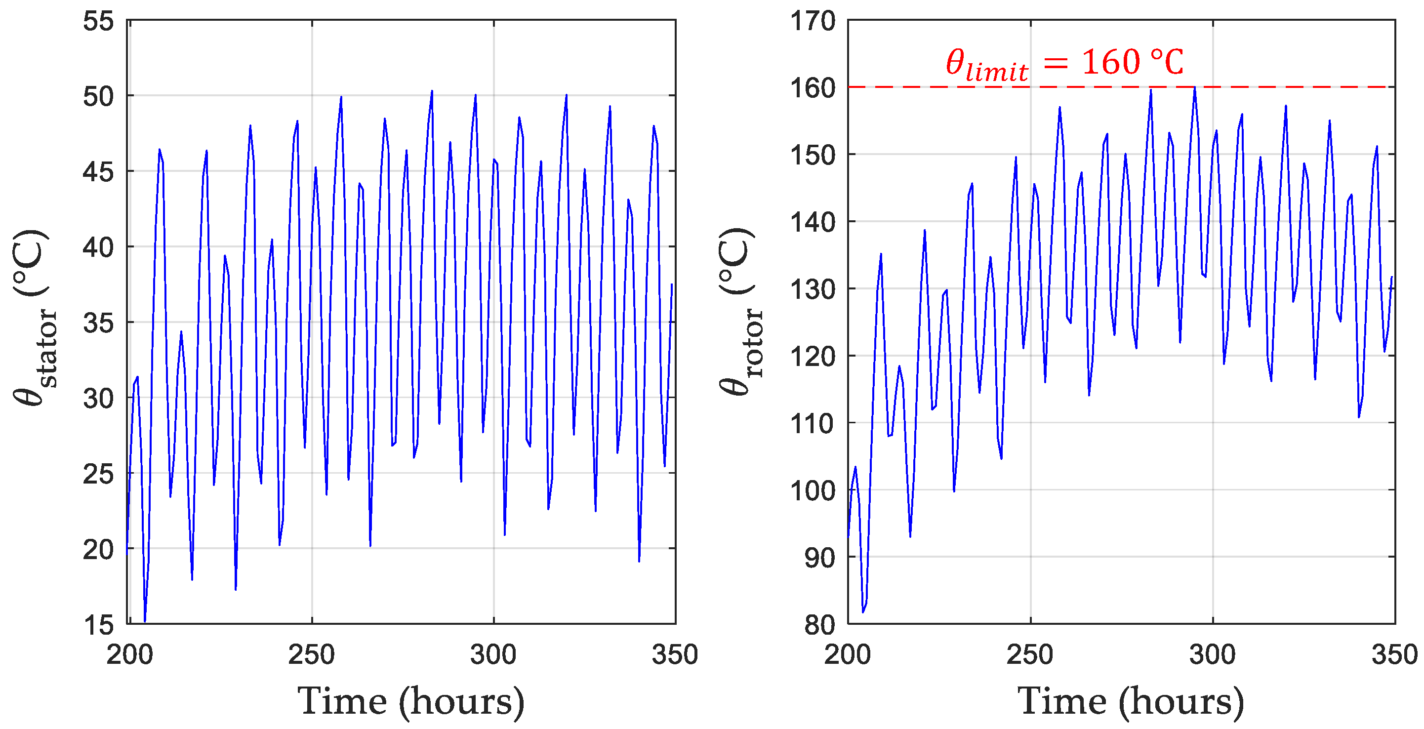
Finally, Figure 11 shows the evolution temperature in the stator and rotor windings during the sequence where the machine is the warmest. This calculation is conducted by solving Equation (42) applied to the thermal network. It can be noted that the optimization algorithm respects the temperature limit even if the steady state is not reached throughout the working cycle.

4.2. 2D Validation

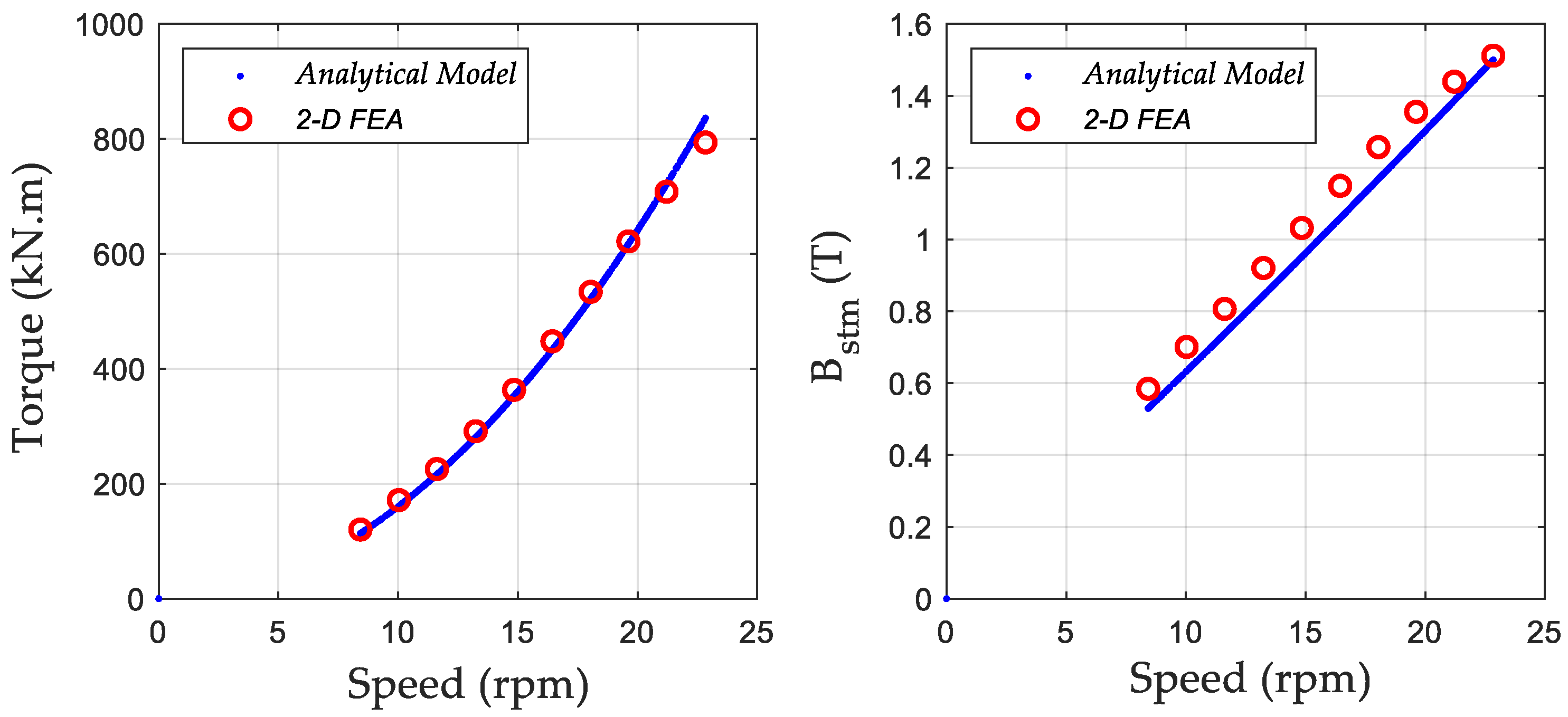
In this section, the analytical model used in our optimization is validated for the optimal selected design. The magnetics field and the electromagnetic torque calculated from the analytic model are compared to their values extracted from a 2D finite element analysis (FEA).

Table 4. Maximum torque and magnetic field at the minimal and the nominal operating points.

Quantity	Min				Max
	AM	2D	Variation	AM	2D	Variation
$B_{stm}$	0.57	0.62	8.06%	1.5	1.58	5.06%
$B_{rtm}$	0.57	0.55	3.64%	1.5	1.46	2.74%
$B_{sym}$	0.56	0.59	5.08%	1.49	1.48	0.68%
$B_{rym}$	0.56	0.59	5.08%	1.5	1.53	1.96%
Torque (MNm)	0.11	0.12	8.3%	0.83	0.79	4.8%

presents these results obtained for the flux densities and the torque at the minimal power and the maximal power. Figure 12 presents this comparison of the torque and the stator teeth for all operating points represented by their mechanical speed. The variations between the models remain always lower than 10%. Such a result validates either the 1D analytical model used and the magnetic saturation constraint.

Table 5. Losses of the optimal generator at the maximal power (2 MW).

	Analytical Model	FEA	Variation
Iron losses in the stator yoke	4.5 kW	4.3 kW	−4.6%
Iron losses in the rotor teeth	10.2 kW	9 kW	−13.3%
Total iron losses	14.7 kW	13.3 kW	−10.5%
Copper losses	67.9 kW

gives the iron losses obtained from the FEA considering the seventh first harmonics of the flux density at nominal power, regularly taken in the teeth and in the yoke. It shows a relatively low influence of the spatial components neglected by the 1D analytical model. Their magnitude remains low compared to the main component, and their location is limited to areas of limited cross-section (the border area between the tooth and yoke).

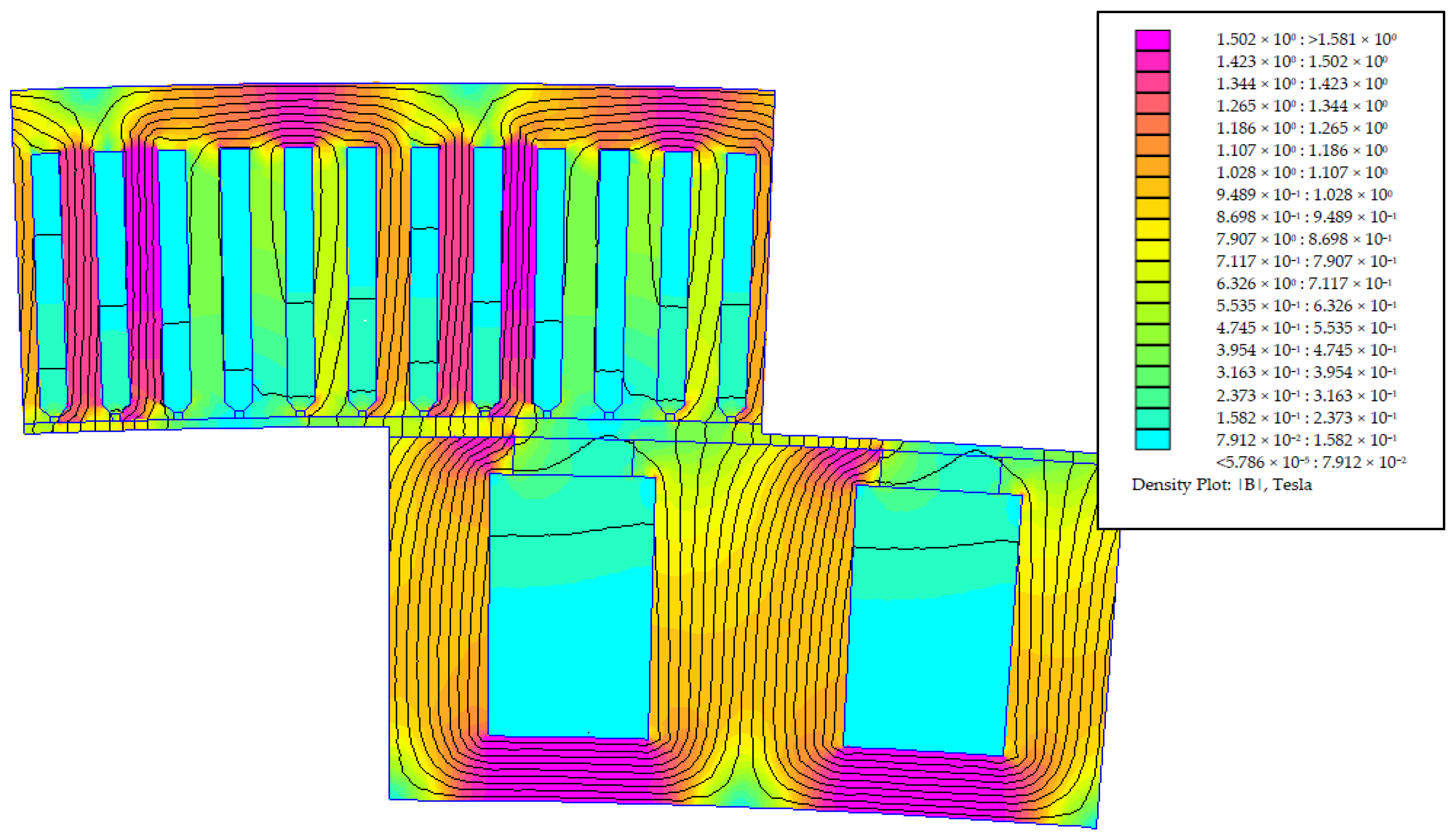
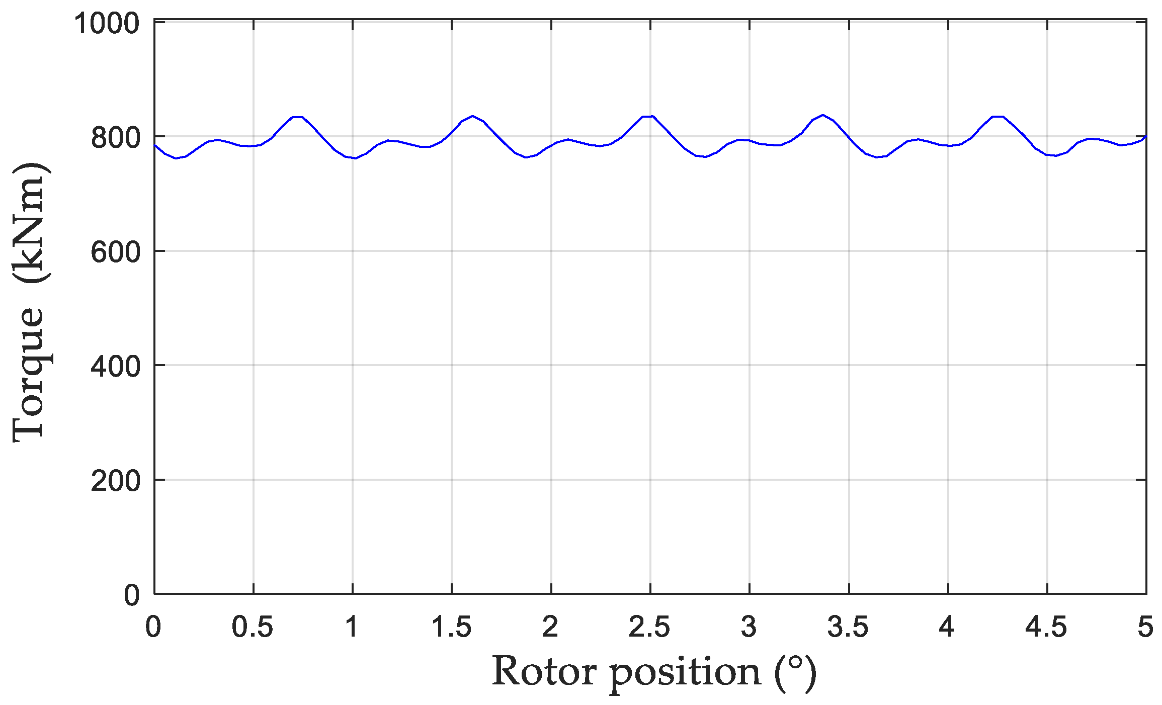
Figure 13 displays the flux lines and flux density obtained with the FEA at the nominal working point. Figure 14 shows the torque evolution with the rotor position at the maximum power. The torque ripple measured is lower than 5% which can be considered satisfactory for a first result.

5. Conclusions

In this paper, we have presented a new method to solve with a reduced computation time the sizing problem of an EESG that works at variable speed and torque. This method is particularly useful and efficient when the machine works at a transient thermal regime. In addition, the method presented allows optimization of the control strategy, optimizing for all operating points of the stator current ($i_d\left(t\right)$ and $i_q\left(t\right))$ and the excitation filed current ($I_f\left(t\right))$, which cannot be conducted by classical solutions. It can be seen that the minimization of electrical losses is achieved by a flux weakening acting on both $i_d$ and $I_f$. For the particular case of the tidal application studied here, a control at $i_d=0$ may be implemented and the flux weakening performed by the excitation filed current alone. The results obtained also showed that the method lead to reduce the mass by 18% compared to a conventional sizing at the nominal operating point while controlling the losses by an optimization of the currents. The FEA shows that, despite a simple 1D magnetic model, the design obtained is already acceptable. Among the possible improvements, the authors work to develop a magnetic model with saturation which will be presented in future works.