Data-Driven State Prediction and Analysis of SOFC System Based on Deep Learning Method

Abstract

A solid oxide fuel cell (SOFC) system is a kind of green chemical-energy–electric-energy conversion equipment with broad application prospects. In order to ensure the long-term stable operation of the SOFC power-generation system, prediction and evaluation of the system’s operating state are required. The mechanism of the SOFC system has not been fully revealed, and data-driven single-step prediction is of little value for practical applications. The state-prediction problem can be regarded as a time series prediction problem. Therefore, an innovative deep learning model for SOFC system state prediction is proposed in this study. The model uses a two-layer LSTM network structure that supports multiple sequence feature inputs and flexible multi-step prediction outputs, which allows multi-step prediction of system states using SOFC system experimental data. Comparing the proposed model with the traditional ARIMA model and LSTM recursive prediction model, it is shown that the multi-step LSTM prediction model performs better than the ARIMA and LSTM recursive prediction models in terms of two evaluation criteria: root mean square error and mean absolute error. Thus, the proposed multi-step LSTM prediction model can effectively and accurately predict and evaluate the SOFC system’s state.

1. Introduction

Human beings are striving to make low-carbonization energy systems and gradually decarbonize them to cope with energy problems and ecological degradation. With the ability to effectively convert chemical energy into electrical energy [1] and the advantages of near-zero emissions, low noise, superior energy efficiency and high power density [2,3,4,5], solid oxide fuel cell (SOFC) technology has huge potential for application in new energy vehicles, distributed power generation and military equipment [6]. Due to the complex coupling relationships in SOFC systems, performance degradation or even failure can easily occur during actual operation, which makes the durability and long-term performance of SOFC system poor, and hinders its large-scale commercialization [7].

To ensure that SOFC systems operate safely and efficiently in the long term, system-level prediction and health management (PHM) is a necessary and effective measure. The prediction and evaluation of the SOFC system operation state is the foundation of the system PHM, which is conducive to control and reduce maintenance costs of the system [8,9]. Therefore, SOFC system state prediction and evaluation is a key prerequisite to extend the working life of the system.

In recent years, there has been an increased interest in the development of prediction strategies for FCs. Various prediction approaches are generally classified into three types: model-based, data-driven and hybrid. As for model-based prognostics, also known as white-box models, mathematical methods are used to establish mechanistic models of FCs to predict the fuel cell states [10,11,12,13,14,15,16]. However, most of these studies are on proton exchange membrane fuel cells (PEMFC) or just SOFC stacks, which are the core component of SOFC systems. No literature, as far as we know, studies prediction methods for SOFC systems. Model-based prediction methods are intuitive and do not require large amounts of experimental data, but it is actually difficult to build an accurate model because the fuel cell is a non-linear, multi-physics (electrochemical, thermal, mechanical, fluidic) and multi-scale (space, time) complex coupled system [17,18,19,20]. Model-based prediction methods are often based on assumptions and approximations, limited by the knowledge of the actual system, which greatly increases the uncertainty of SOFC system prediction, and one system corresponds to one model, making the model poorly adaptable.

In contrast, data-driven prediction is called a black box model. It learns the system behavior from the system’s sensor monitoring data and predicts the future system state without any physical understanding of the system behavior and complex mathematical equations. Data-based prediction models tend to have better adaptability and accuracy and are easy to implement, but they require a large amount of SOFC system monitoring data. Such methods convert historical state-monitoring data into corresponding information and system behavior model through statistical techniques or machine learning techniques, such as the artificial neural network model [21], the hidden semi-Mark model [22], the Elman neural network model [23], the similarity of phase space trajectory [24], and the neural network autoregressive model [25]. From the literature review, the research on data-driven prediction methods for SOFC systems is still limited and far less than that for PEMFC system [26,27,28,29,30,31,32]. Moreover, the data used in many proposed prediction models are simulation data, not actual experimental data, and the prediction is often a one-step prediction, which is often limited to analysis and has little application value.

Hybrid methods are methods that integrate model-based and data-driven approaches. Dolenc et al. [33] used a hybrid approach to estimate the trend of future degradation and the remaining useful life (RUL) of the SOFC. Firstly, the author developed a lumped stack model, and then used an unscented Kalman filter to estimates the current area specific resistance (ASR) value. Then the authors used a linear Kalman filter to recursively identify the drift model, which is used to describe the time evolution in the ASR, to predict the future time evolution in the ASR and finally obtained the RUL. Obviously, the object of this research is only the stack, a core component of the SOFC system.

Based on the above discussion, the main research gaps are as follows:

• The mechanism of the SOFC system has not been fully revealed. Model-based prediction methods are often based on assumptions and approximations. These methods have low accuracy and are poorly adaptable, and these studies tend to focus on SOFC stacks rather than SOFC systems.
• Current data-based SOFC prediction studies are often single-step prediction studies, which do not meet the requirements of practical applications. Moreover, many studies use inaccurate simulation data rather than high-quality experimental data.

The SOFC system state prediction problem can be viewed as a time series prediction problem. The recurrent neural network (RNN) is an artificial neural network with the nodes being connected in a directed loop. Its internal state can show dynamic temporal behavior, which is very effective for processing data with sequential features. The Long Short-Term Memory network (LSTM) is a special kind of RNN that avoids the problems of gradient exploding and gradient vanishing of the RNN [34]. The simple LSTM network structure can handle the problem of time series prediction, but it is usually used for one-step prediction and has little application value in SOFC system state prediction. Recursive prediction using LSTM network structure can achieve multi-step prediction, but this operation is more complicated and can only perform single-series prediction single sequence prediction, and the prediction accuracy is not satisfactory.

In this paper, a deep learning model for state prediction of SOFC systems based on LSTM cells is developed. The model adopts a two-layer LSTM structure, which supports multiple sequence feature inputs and flexible multi-step prediction outputs. Firstly, the raw experimental data is simply filtered to remove redundant and invalid features, and the sequence forward selection (SFS) method is used to obtain the best feature subset to reduce the computational complexity, and some preprocessing is performed to fit the prediction model. Then, the multi-step LSTM prediction model is established to predict the state of the SOFC system (such as output voltage value). Finally, specific evaluation criteria are used to evaluate the prediction accuracy of the multi-step LSTM prediction model and compare it with the traditional ARIMA model and the LSTM recursive prediction model. The main contributions of this paper can be listed as follows:

• A data-based multi-step LSTM state prediction model is proposed for the first time to perform state prediction for SOFC systems.
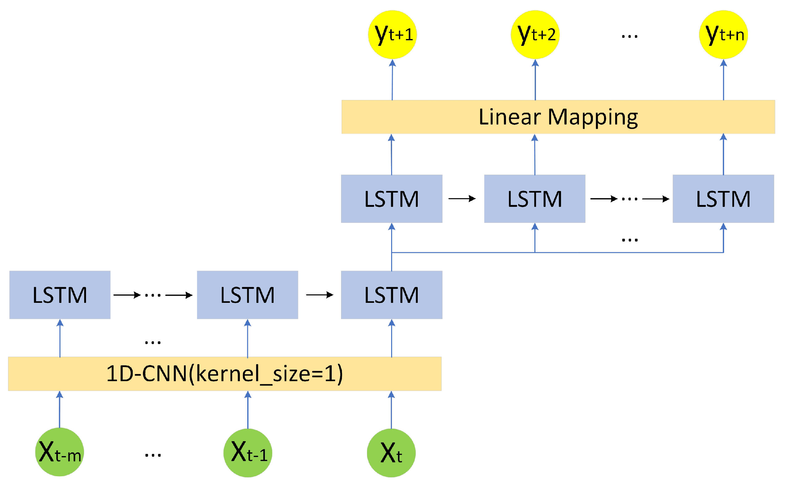
• The unique two-layer LSTM structure of the proposed model allows the model to support multiple sequence feature inputs and flexible multi-step prediction outputs.
• Experiments were conducted on a 1kW SOFC power generation system, and the proposed model was trained and tested with the experimental data.

This paper is organized as follows. Section 2 introduces the structure of the SOFC system in which the experiments are conducted, system experimental scheme and the raw monitoring data. Section 3 puts forward the prediction framework of the multi-step LSTM state prediction of the SOFC system. Section 4 presents the state prediction results and the comparison of different prediction models and the concluding remarks are introduced in Section 5.

2. Experimental Scheme and Data Implementation

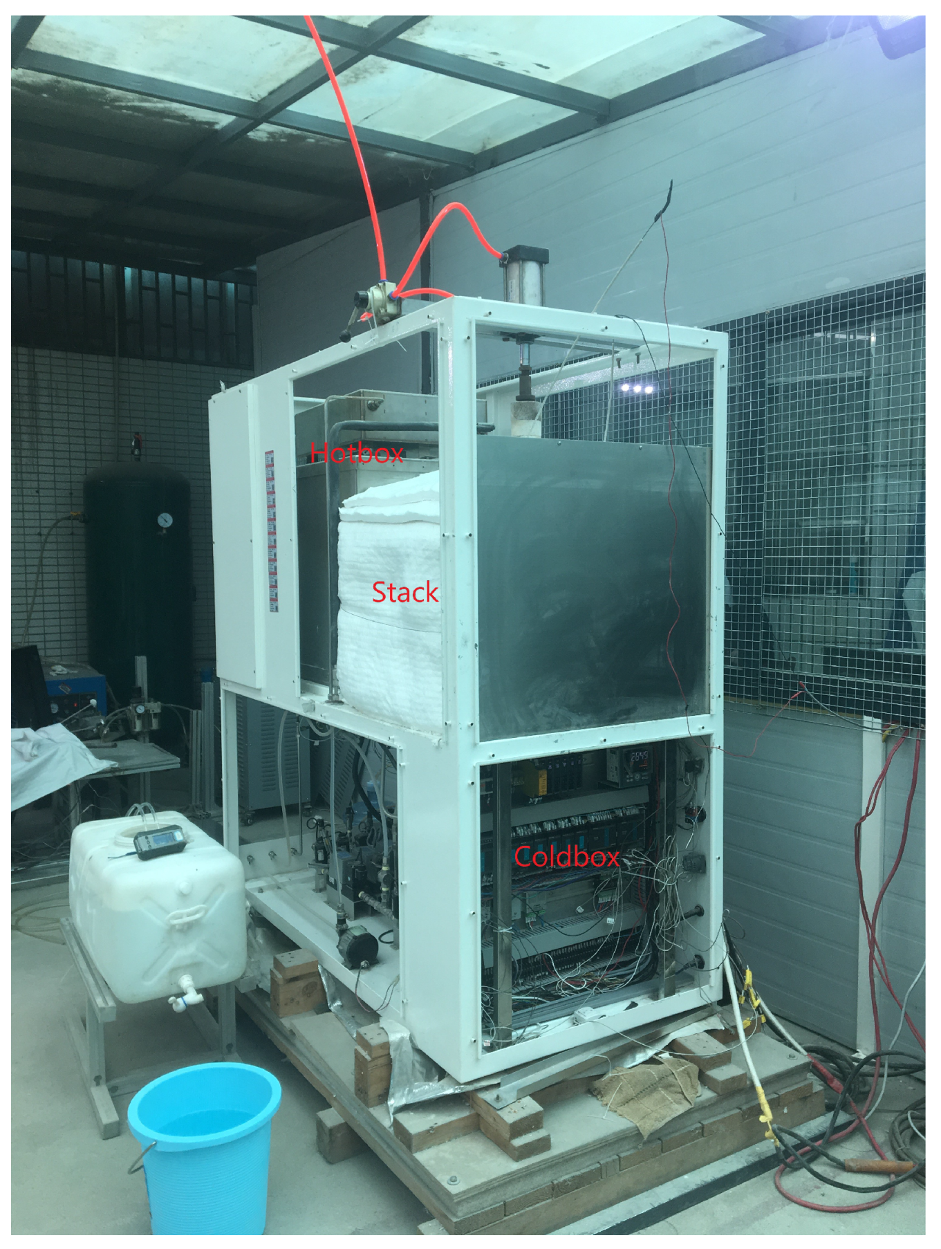
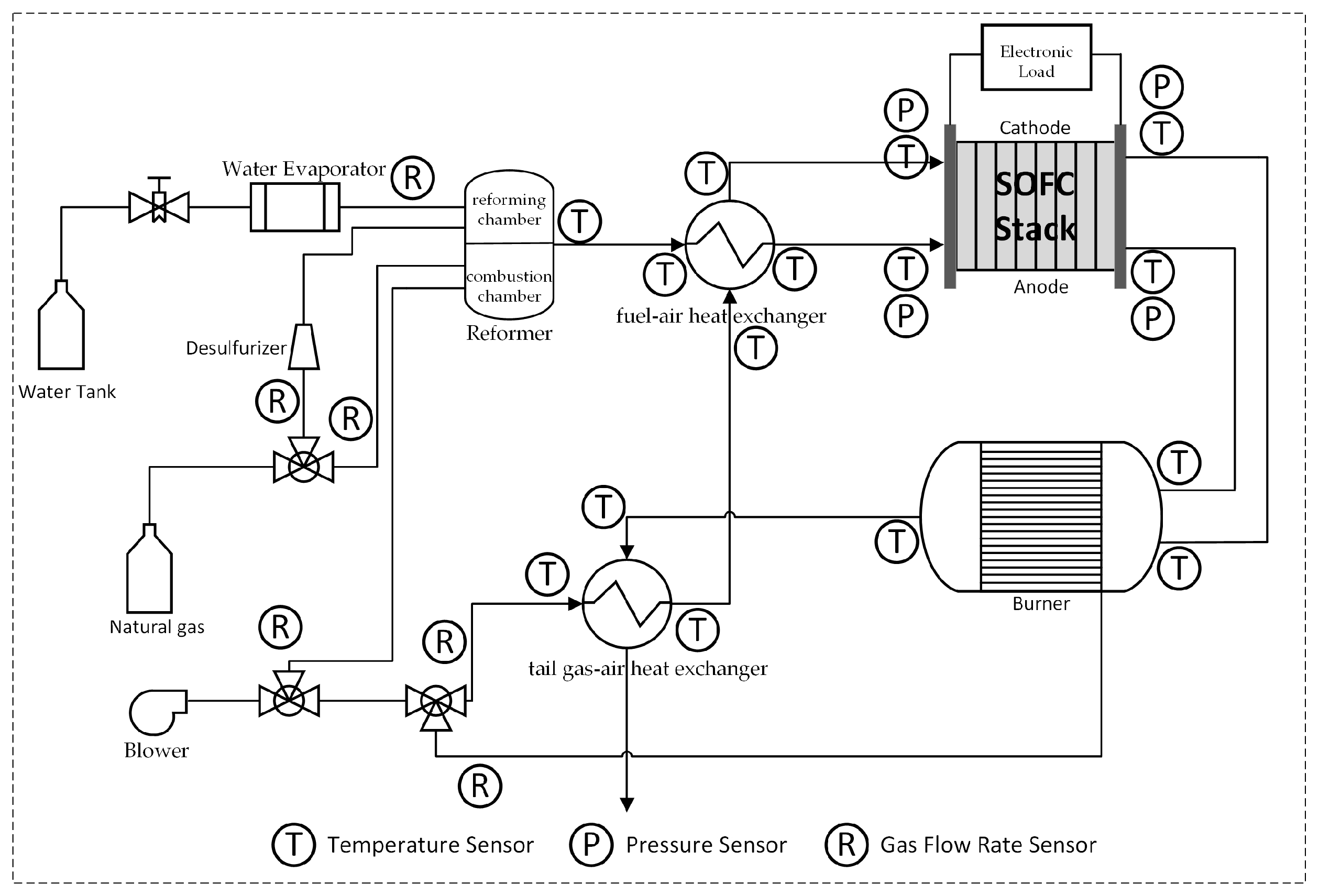
2.1. System Structure

The experimental device for this study is a 1 kW SOFC power generation system [35], as shown in Figure 1. The SOFC system, which has a good fuel flexibility, directly uses hydrocarbon fuels to generate electricity [36] and the most common are methane and hydrogen. In this experiment, the fuel for the 1 kW SOFC power generation system is methane, which is reflected in the auxiliary components of the SOFC system. As shown in Figure 2, a complete SOFC system is composed of its core component SOFC stack and other equipment supported by the balance of plant (BOP). There are multiple single cells in a SOFC stack with the anode connected to the fuel and the cathode connected to oxygen or air. The following electrochemical reactions will occur in the single cell to convert chemical energy into electrical energy.

$${\mathrm{H}}_2+\frac{1}{2}{\mathrm{O}}_2\to {\mathrm{H}}_2\mathrm{O}+\mathrm{heat}+\mathrm{electricity}$$

(1)

$$\mathrm{CO}+\frac{1}{2}{\mathrm{O}}_2\to {\mathrm{CO}}_2+\mathrm{heat}+\mathrm{electricity}$$

(2)

The stack used in the system consists of 27 single cells with a size of 15 × 15 cm² and an effective working area of 13 × 13 cm². There is a cross-flow structure in the flow field of the stack. The BOP components of SOFC system mainly include reformer, heat exchanger, exhaust burner, water evaporator, blower, electronic load, controller, etc. The SOFC system operates in a high-temperature environment. In the fuel path, part of 99.5% pure methane is mixed with the water vapor at the outlet of water evaporator and enters the reformer reforming chamber for reforming reaction, and the other part is burned with air in the reformer combustion chamber to provide continuous high-temperature conditions of 600–700 °C for reforming reaction. The reforming reaction produces hydrogen (H₂) and carbon monoxide (CO), which then enter the fuel–air heat exchanger to control the temperature difference between cathode and anode gas. After that, the fuel gas enters the anode of the high-temperature SOFC stack and reacts, completing the conversion from chemical energy to electric energy, and the unreacted gas enters the exhaust burner. In the air path, part of the air enters the combustion chamber of the reformer, part of the air passes through the tail gas–air heat exchanger to exchange heat with the high-temperature tail gas, which comes out of the exhaust burner, to raise the air temperature, and part of the air directly enters the exhaust burner to ensure full combustion of the unreacted fuel gas. The high temperature air at the outlet of the tail gas–air heat exchanger passes through the fuel–air heat exchanger and enters the cathode of the SOFC stack. Similarly, unreacted air passes into the exhaust burner and is mixed with unreacted fuel gas to generate high-temperature tail gas. The high-temperature tail gas can be directly discharged after passing through the tail gas–air heat exchanger.

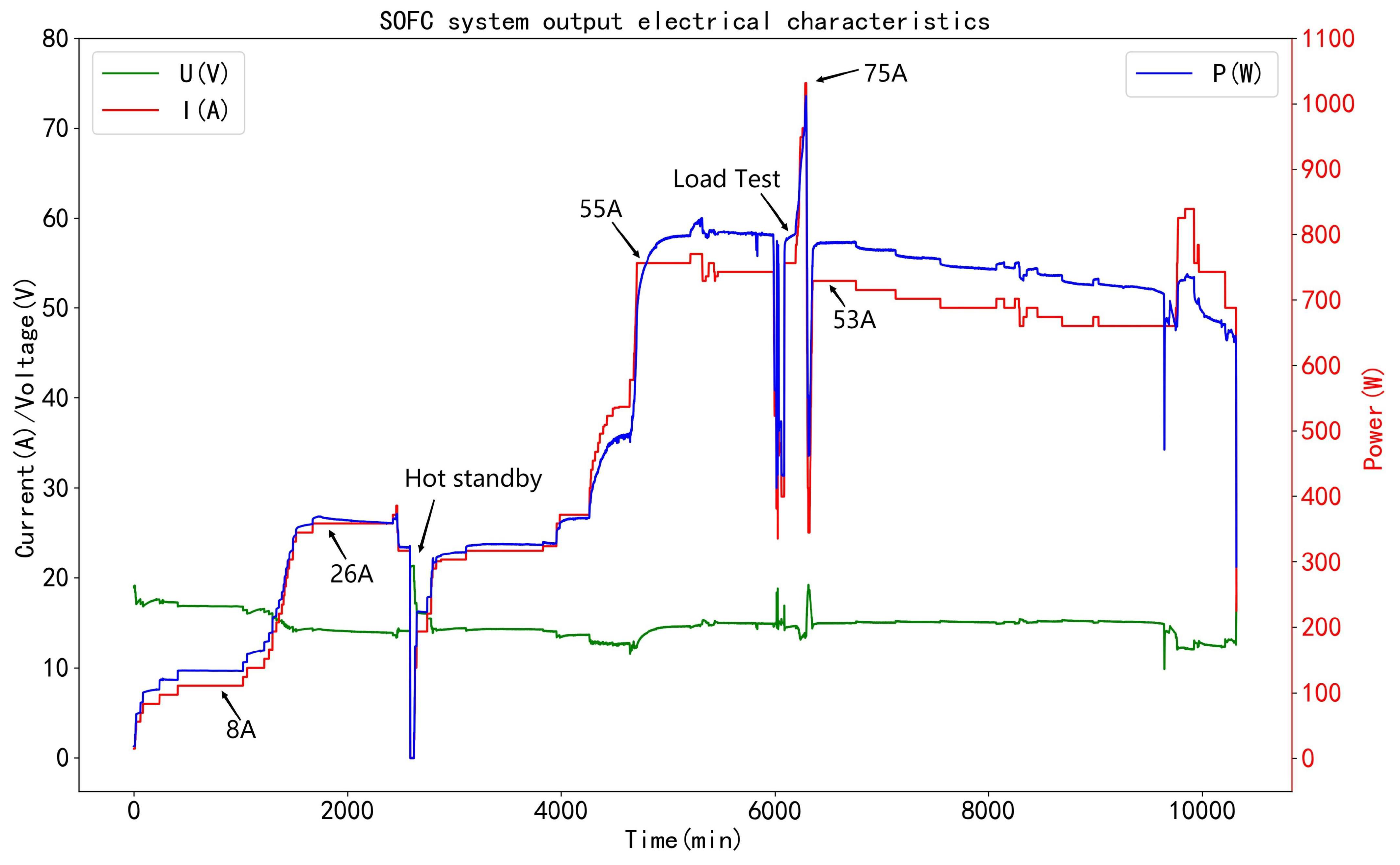
2.2. Experimental Scheme and Data Collection

As the SOFC stack temperature rises to a temperature range that can generate electricity, the electronic load is turned on, and the SOFC system starts to generate electricity. With a sudden increase of the load, there may not be enough fuel and heat available to the SOFC system to maintain that it can operate under the new load condition [37]. Therefore, the electronic load is slowly increased, giving the system enough time to react. During this process, the output current of the SOFC system slowly rises and the system output voltage gradually decreases from the open-circuit voltage. During the first current rise phase, the system output current is maintained at 8 A and 26 A, respectively, for a period of time, and then the system enters the hot standby state, which means that the output electrical characteristics behave as open-circuit voltage and 0 A current and that the stack stays at a high temperature. When the hot standby state ends, the system enters the second current rising stage, and the output current is gradually pulled up to 55 A. Then, the load test is performed on the SOFC system and the peak of the system output current rises to 75 A. Then the load test ends, and the system current recovers to 53 A and enters the long-term stable operation phase. The system stack temperature remains relatively stable, while the output current shows a downward trend, and the SOFC stack is in a degradation period. During the whole experiment, the output electrical characteristics of the SOFC system are shown in Figure 3.

During the experiment, a total of 82 original variables were monitored, of which 8 were Boolean variables and 74 were numerical variables. The numerical variables are mainly current, voltage, power, temperature, pressure and gas flow rate, etc. The data acquisition included the SOFC system stack and various BOP components of the SOFC system. The sampling time of each group of data was 1s, and a total of 629,873 groups of data were collected. As one of the most important and valuable state characteristics [38], the output voltage of the SOFC system will be used as a typical demonstration of state prediction in this paper.

3. State Prediction of the SOFC System

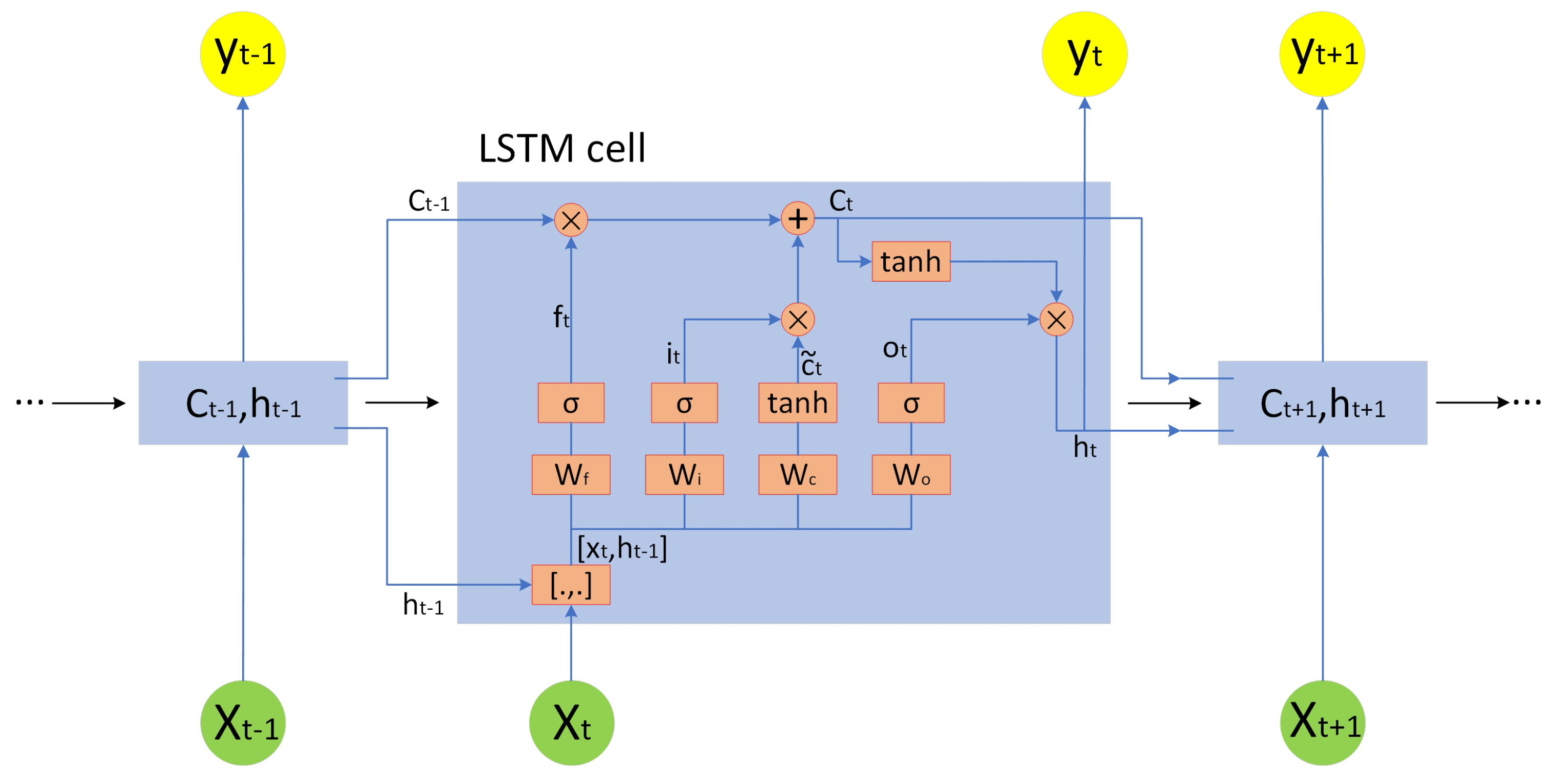
3.1. LSTM Architecture

LSTM networks were first proposed in 1997 [39]. Compared to traditional RNNs, each LSTM cell adds a “processor” consisting of a forget gate, an input gate and an output gate [40] to filter the information. The forget gate determines the extent to which the LSTM cell can remember the cell state of the previous moment; the input gate determines the extent to which the input of the current cell affects the cell state; and the output gate determines the extent to which the current cell state affects the output value of the cell. Like the traditional RNN, during the gradient backpropagation of LSTM, the gradient is not only propagated between the neural network layers, but also between the recurrent neurons in the hidden layer. However, the gradient of RNN becomes too large or too small when the time series is too long and the gradient propagates forward in the recurrent neurons of the hidden layer, which is called gradient exploding and gradient vanishing. The unique structure of the LSTM cell can solve the gradient exploding and gradient vanishing problems of RNN effectively.

As shown in Figure 4 and Figure 5, consisting of an input layer, a hidden layer and an output layer, the output of a simple LSTM neural network is either a combination of the outputs of each cell or the output of the last cell. When the LSTM neural network’s output is a combination of the output of each cell, the model structure fixes the time step of the output, that is, the historical features of n time steps are used to predict future n time steps of the outcome. When the LSTM neural network’s output is the output of the last cell, only one-step prediction can be performed, that is, the historical features of n time steps are used to predict future 1 time steps of the outcome. Simple LSTM neural networks are usually used to make single-step predictions and cannot make flexible multi-step predictions.

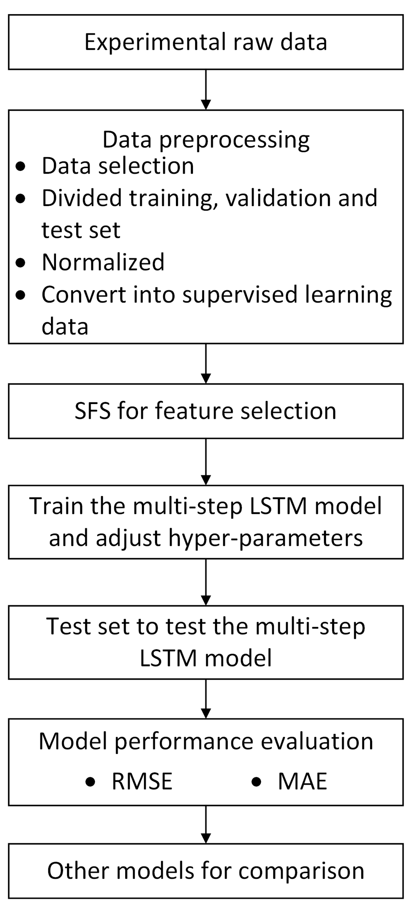
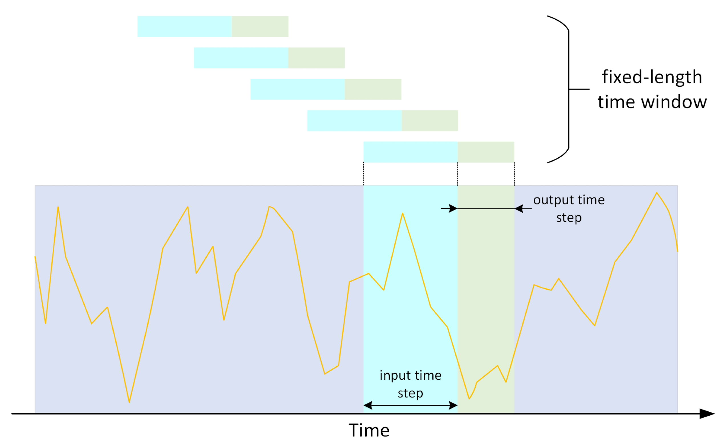
3.2. Multi-Step LSTM State Prediction Framework

The framework of the multi-step LSTM state prediction model is shown in Figure 6. The specific contents will be introduced in detail below.

3.2.1. Data Preprocessing

The sampling time of the raw experimental data is 1 s, so the data is too dense and will lead to a heavy computational burden. Considering that a sampling time of 1 min does not appear too data-intensive but allows to retain enough experimental data for use, a suitable start-up time should be chosen to collect a valid set of data at one-minute intervals after removing invalid data before the SOFC generation system is started and after it is switched off. In this way, 10,323 groups of data were selected from the raw data. There were 82 monitored variables in the raw data, of which 8 boolean variables were not helpful for system state prediction and should be discarded. The remaining 74 numerical variables also had plenty of invalid variables, especially a large number of redundant temperature variables, because in the experiment, temperature sensors were arranged at the inlet and outlet of almost every component of the SOFC system. Therefore, as shown in

Table 1. The preliminarily selected variables of the SOFC system.

	Variables
Output voltage	Output current	Cathode air flow rate
Bypass air flow rate	Methane flow rate	Input methane pressure
Cathode air pressure	Bypass air pressure	Anode input pressure
Cathode input pressure	Anode output pressure	Cathode output pressure
Reformer temperature	Anode inlet temperature	Cathode inlet temperature
Anode outlet temperature	Cathode outlet temperature	Fuel inlet temperature of burner
Air inlet temperature of burner	Burner temperature	Fuel-air heat exchanger temperature

, according to the prior knowledge of the SOFC system and experimental experience, 21 system state variables were preliminarily reserved.

Then, the data need to be divided into three sets: training set (first 7000 groups of data), validation set (next 1000 groups of data) and test set (the rest of the data). For the purpose of adapting to the characteristics of the LSTM neural network, all data need to be normalized by min-max scaling, that is, 21 system state variables should be processed by the following formula respectively.

$$X_{scaled}=\frac{X-Min}{Max-Min}$$

(3)

where $X_{scaled}$ is the normalized system state variable, X is the raw state variable, and $Max$ and $Min$ denote the maximum and minimum values of the state variable respectively.

Data leakage tends to occur during the data pre-processing phase. Therefore, the $Min$ and $Max$ used for the normalization of the validation set and the test set should be the $Min$ and $Max$ of the training set. Time sequence data cannot be used directly for trainning the model, so it is necessary to convert time sequence data into supervised learning data with input data and output data using a fixed-length sliding time window (Figure 7).

3.2.2. SFS for Feature Selection

Sequential forward selection (SFS) is a search method that generates a subset of features during the feature selection process. In this experiment, the RMSE of the multi-step LSTM prediction model is used as the evaluation criterion, and the search starts with that feature subset as a empty set. Add one feature to this feature subset each time, and use the features in the feature subset to train the multi-step LSTM prediction model until the evaluation function reaches an optimal value. Finally, an optimal feature subset with seven features is obtained and they are output voltage, output current, input methane pressure, cathode air pressure, anode input pressure, anode output pressure and cathode output pressure.

3.2.3. Multi-Step LSTM State Prediction Model

As shown in Figure 8, the multi-step LSTM prediction model adopts a two-layer LSTM structure, in which the output of the last cell of the first LSTM layer is the input of all cells in the second LSTM layer. In this way, the time steps of input and output can be flexibly adjusted to realize flexible multi-step prediction. The prediction model also adds a one-dimensional convolution layer with a kernel size of 1 between the input layer and the first LSTM layer, which is to adjust the input data’s feature dimension of the LSTM layer without changing the time series characteristics of the input data.

3.3. Other Models for Comparison

The Autoregressive Integrated Moving Average Model (ARIMA) is a well-known model for time series forecasting. ARIMA is a model established by eliminating trend and seasonality to obtain time series data that is considered stationary, and then regressing the dependent variable only on its lagged values and the present and lagged values of random error terms [41]. An ARIMA model is usually specified by a tuple (p, d, q), with p being the order of the autoregressive term, q the order of the random error moving average term, and d the number of difference operations when the time series becomes a stationary series. The classical ARIMA model is a single sequence prediction model. Therefore, when the ARIMA model predicts the output voltage of a SOFC system, only the output voltage is valuable, and other variables should be discarded.

While simple LSTM neural network models are usually used for single-step prediction, we can achieve multi-step prediction by recursive prediction. Recursive multi-step prediction is still essentially simple single-step prediction. The recursive strategy is to use the predicted value as a feature and then make a single-step prediction again. Recursive prediction accumulates prediction errors due to the use of predicted values instead of true values. As the prediction time step increases, the predictive performance of the model may rapidly deteriorate. Similar to the ARIMA model, the LSTM recursive prediction model is also a single sequence model.

3.4. Evaluation Criteria of Prediction Performance

In this study we use two evaluation criteria to assess the prediction performance of the SOFC system state prediction model: root mean square error (RMSE) and mean absolute error (MAE). When the values of MAE and RMSE are smaller, we consider that the more accurate the predicted value is and the smaller the error is.

$$\mathrm{RMSE}=\sqrt{\frac{1}{N}\sum _1^N{(y\left(t\right)-\widehat{y}\left(t\right))}^2}$$

(4)

$$\mathrm{MAE}=\frac{1}{N}\sum _1^N|y\left(t\right)-\widehat{y}\left(t\right)|$$

(5)

where $y\left(t\right)$ denotes the measured real value of the SOFC system output voltage, $\widehat{y}\left(t\right)$ is the predicted voltage value of the prediction model output, and N is the total number of predicted outputs.

4. Results and Discussion

4.1. Hyper-Parameters of the Multi-Step LSTM Prediction Model

In this experiment, mean squared error (MSE) regression loss and Adam optimizer are used during model training. We set the number of output channels of the 1D convolutional layer to 32 and the hidden size of both LSTM layers to 32. In addition, batch size and learning rate are two important hyper-parameters of the model. We study the effect of these two hyper-parameters on the RMSE and MAE of the validation set when they are set to different values, and the results are presented in

Table 2. Results of validation set prediction with different learning rates.

Batch Size	Learning Rate	RMSE	MAE
10	0.001	0.0290	0.0233
	0.0001	0.0239	0.0136
	0.00001	0.0307	0.0223

and

Table 3. Results of validation set prediction with different batch sizes.

Learning Rate	Batch Size	RMSE	MAE
0.0001	30	0.0314	0.0224
	20	0.0240	0.0156
	10	0.0239	0.0136
	5	0.0226	0.0134

. The number of training epochs for the model is fixed at 30, and the input and output time steps are 20 and 10 respectively.

When the learning rate is 0.0001, the RMSE and MAE are 0.0239 and 0.0136 respectively, which showed the best performance for the validation set prediction. In contrast, when the learning rate is 0.001 or 0.00001, the prediction performance on the validation set decreases. It can be seen that too large or too small a learning rate has a negative impact on the prediction performance of the multi-step LSTM prediction model. When the batch size is varied among 30, 20, 10 and 5, the smaller the batch size, the smaller the RMSE and MAE of the validation set, but also the longer the training time of the model. We consider a learning rate of 0.0001 and a batch size of 10 to be appropriate.

4.2. Performances Analysis Based on Comparison

To evaluate the performance of the multi-step LSTM prediction model on multi-step prediction, we use the model to predict the output voltage of the SOFC system on the test set for 10 time steps, 30 time steps and 60 time steps respectively, that is, to predict the output voltage in the next 10 min, 30 min and 60 min respectively. To eliminate the fortuity of the model prediction results, we train the model five times and take the average of the five prediction results. The predicted results are shown in Figure 9.

As can be seen from Figure 9, the prediction evaluation criteria RMSE and MAE for the test set are both less than 0.5, which shows that there is excellent prediction performance when the multi-step LSTM prediction model is used to predict the output voltage of the SOFC system. However, it is clear from the variation of the performance evaluation criteria that for the multi-step LSTM prediction model the prediction performance decreases as the number of prediction time steps increases.

It can be noticed that the RMSE of the test set is significantly greater than the MAE regardless of the prediction time step. The analysis shows that at approximately 9700 min, the operating conditions change dramaticall, y and there is a significant drop in the output voltage of the system. During the shift in operating conditions, a large error in prediction occurred. Because the RMSE squares each error, some of the larger errors have a greater impact on the RMSE value, which results in the RMSE being significantly larger than the MAE value.

For the purpose of verifying the superiority of the proposed model, we compare its prediction results with those of the LSTM recursive prediction model and the ARIMA model. The results are summarized in

Table 4. Comparison results of the three models at different output time steps.

Model	10 Time Steps		30 Time Steps		60 Time Steps
	RMSE	MAE	RMSE	MAE	RMSE	MAE
multi-step LSTM	0.1952	0.0462	0.2644	0.1066	0.3444	0.1691
ARIMA	0.2222	0.0588	0.3272	0.1121	0.3877	0.1756
recursive LSTM	0.2144	0.0941	0.4117	0.3181	0.6731	0.5403

. Figure 10 and Figure 11 show the comparison results based on RMSE and MAE respectively. It should be noted that the ARIMA model parameters are determined using the Bayesian Information Criterion (BIC), with p and q taking values ranging from 0 to 15, and its parameters are finally determined to be (13, 1, 2).

Comparing the performance evaluation criteria of the three models at different time steps, whether RMSE or MAE, the multi-step LSTM prediction model has the lowest value. The comparison results demonstrate the significant advantage of the proposed multi-step LSTM prediction model for the SOFC system state prediction problem.

Although slightly inferior to the proposed multi-step LSTM prediction model, the ARIMA model also performs well on the SOFC system state prediction problem. This is mainly because the operating conditions of the SOFC system do not change frequently in the test set and the system output voltage is generally stable, which is a prerequisite for the ARIMA model to make reliable predictions. However, the disadvantages of the ARIMA model are that it can only perform single-sequence prediction, cannot utilise multi-dimensional features, and can basically only capture linear relationships, not non-linear relationships, which limits the application of the ARIMA model to the SOFC system state prediction problem.

We can notice that when the output time step is 10, the performance of the LSTM recursive prediction model is not significantly inferior to the other two models. However, when the output time step is 60, the RMSE and MAE of the LSTM recursive prediction model increase by 214% and 474% respectively, while those of the multi-step LSTM prediction model increase by 76% and 266% respectively, and those of the ARIMA model increase by 74% and 199% respectively, making the LSTM recursive prediction model’s RMSE and MAE significantly greater than these two criteria for the other two models. The performance of the LSTM recursive prediction model decreases rapidly with increasing prediction time steps because recursive prediction will accumulate prediction errors, incorrectly giving a large upward or downward trend to the generally stable system output voltage in the test set. In addition to the disadvantages caused by recursive prediction, the LSTM recursive prediction model can only perform single-sequence prediction too.

Based on the present findings, the proposed framework of SOFC system state prediction based on multi-step LSTM prediction model can be considered as effective and has application value.

5. Conclusions

Prediction studies of SOFC systems are one of the most important initiatives to ensure their efficient and long-term operation. Unlike common prediction studies based on mechanistic models, in this paper, a state prediction framework of the SOFC system based on the multi-step LSTM prediction model is proposed. Experimental data with 82-dimensional features from a 1kW SOFC system are used to validate the proposed model. Meanwhile, the proposed model is compared with the LSTM recursive prediction model and the ARIMA model. The main conclusions obtained are as follows:

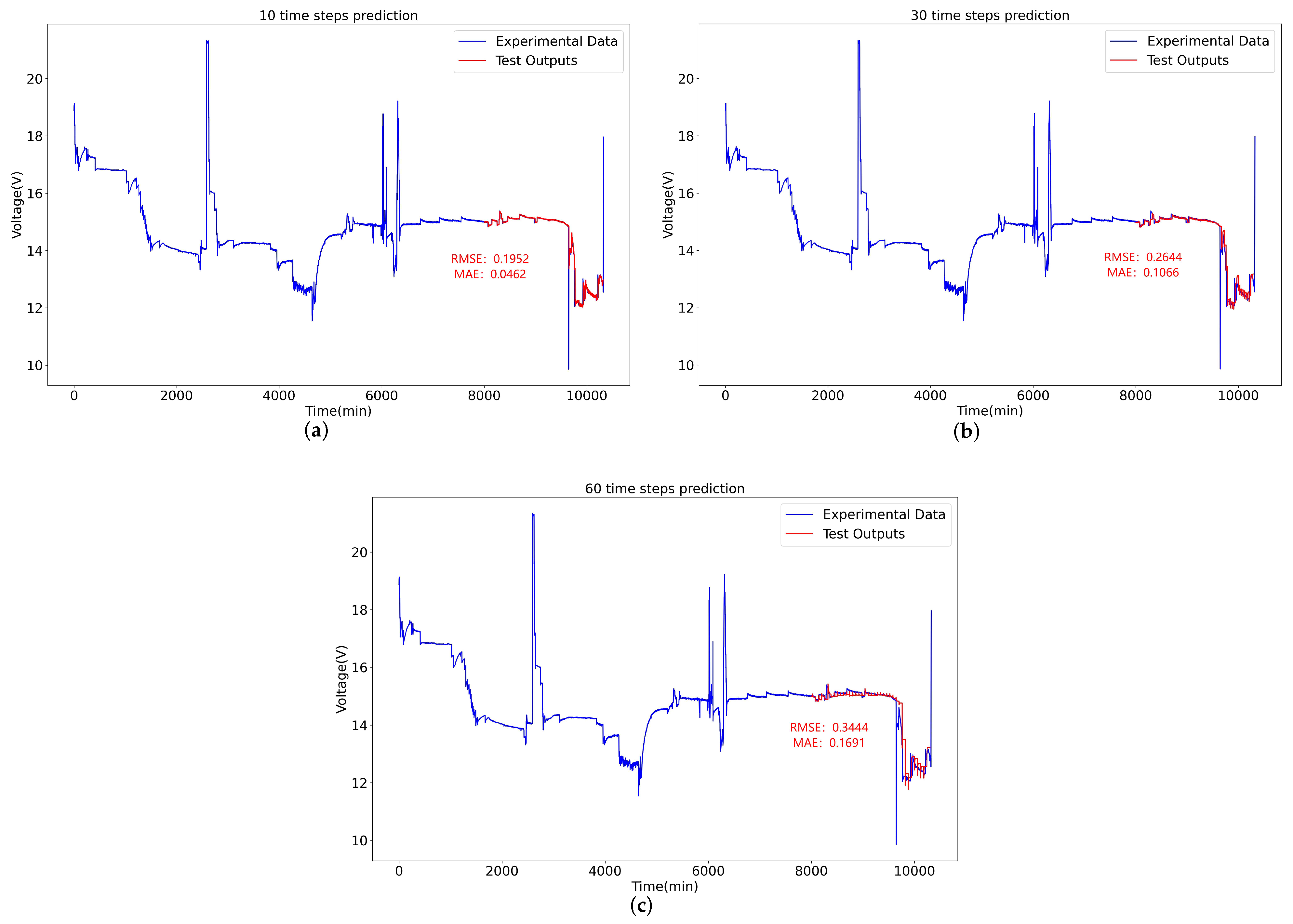
• RMSE and MAE of the multi-step LSTM prediction model on the test set are both less than 0.5 indicating that the model can learn the state properties of the system and predict system’s future state based on the experimental data;
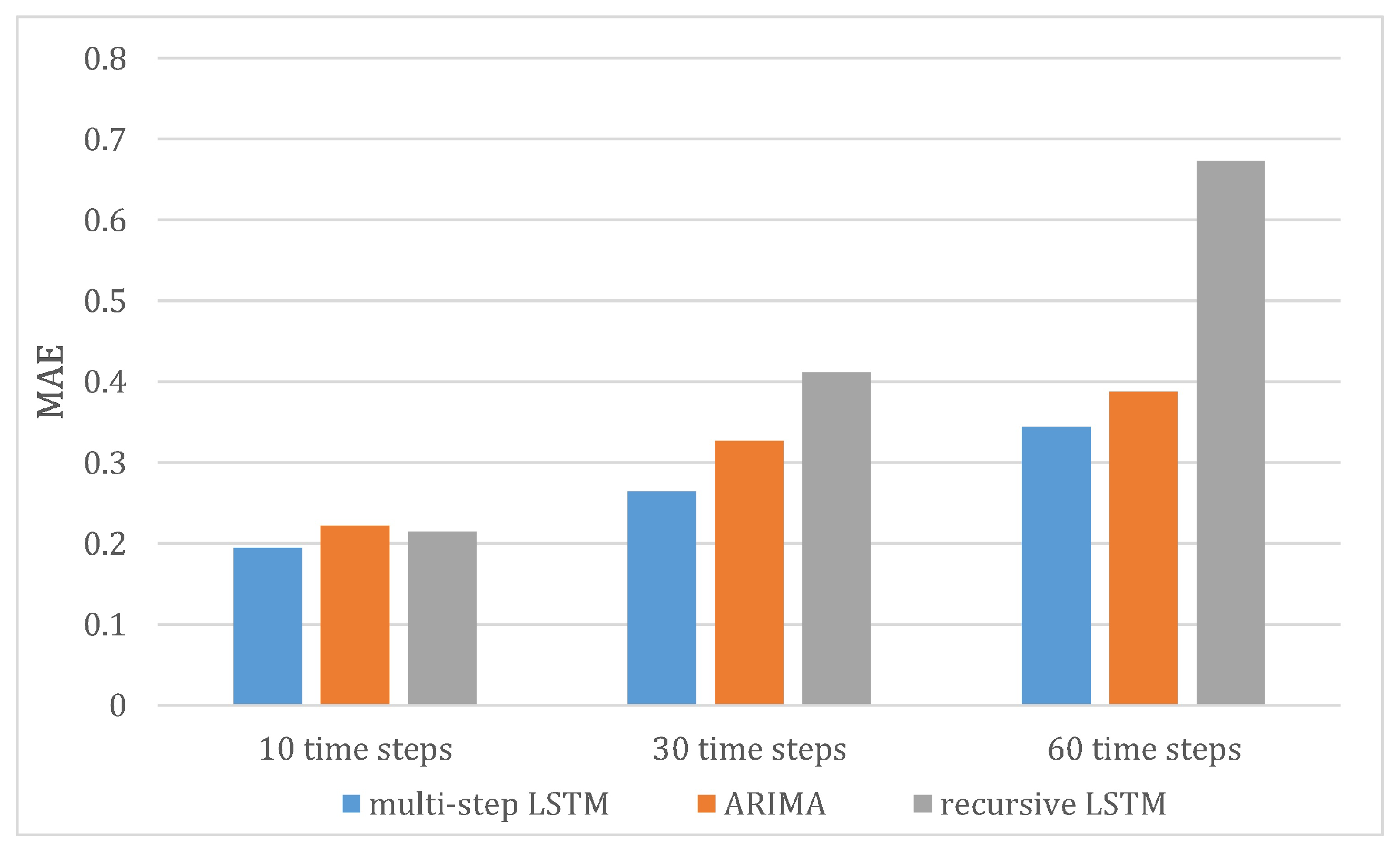
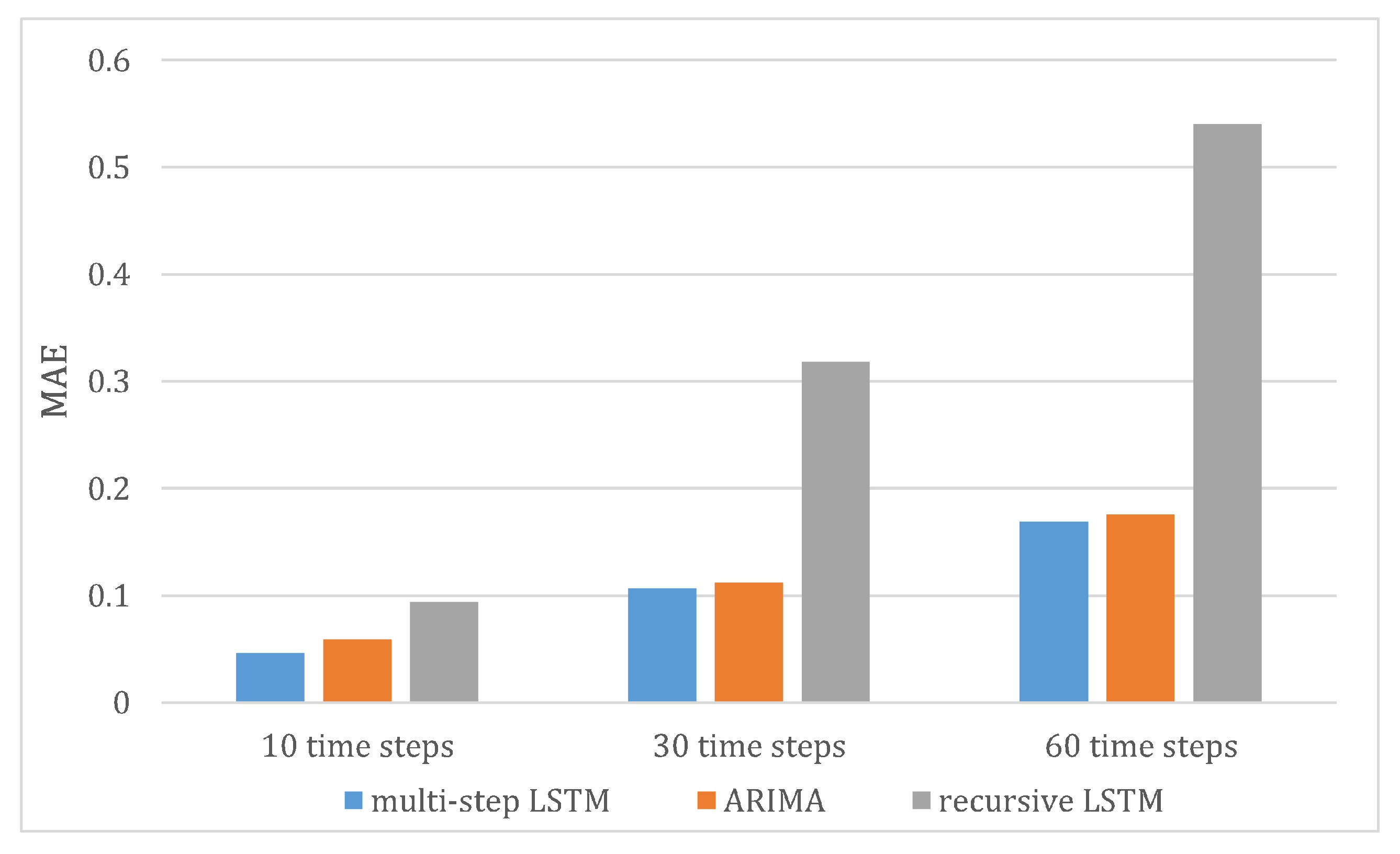
• The multi-step LSTM prediction model allows flexible adjustment of the output time step, and the prediction performance of the model decreases as the number of output time steps increases;
• The comparison results of the three models show that the multi-step LSTM prediction model has excellent prediction performance in the multi-step prediction of SOFC system states, outperforming the other two models.

In this study, the SOFC system output voltage was selected as the predicted state variable. In future studies, other system state variables will be considered as targets for prediction.

References

1. Yang, B.; Guo, Z.; Wang, J.; Wang, J.; Zhu, T.; Shu, H.; Qiu, G.; Chen, J.; Zhang, J. Solid oxide fuel cell systems fault diagnosis: Critical summarization, classification, and perspectives. J. Energy Storage 2021, 34, 102153. [Google Scholar] [CrossRef]
2. Damo, U.M.; Ferrari, M.L.; Turan, A.; Massardo, A.F. Solid oxide fuel cell hybrid system: A detailed review of an environmentally clean and efficient source of energy. Energy 2019, 168, 235–246. [Google Scholar] [CrossRef] [Green Version]
3. Wu, X.L.; Xu, Y.W.; Xue, T.; Shuai, J.; Jiang, J.; Deng, Z.; Fu, X.; Li, X. Control-oriented fault detection of solid oxide fuel cell system unknown input on fuel supply. Asian J. Control. 2019, 21, 1824–1835. [Google Scholar] [CrossRef]
4. Xu, H.; Ma, J.; Tan, P.; Chen, B.; Wu, Z.; Zhang, Y.; Wang, H.; Xuan, J.; Ni, M. Towards online optimisation of solid oxide fuel cell performance: Combining deep learning with multi-physics simulation. Energy AI 2020, 1, 100003. [Google Scholar] [CrossRef]
5. Yang, B.; Wang, J.; Zhang, M.; Shu, H.; Yu, T.; Zhang, X.; Yao, W.; Sun, L. A state-of-the-art survey of solid oxide fuel cell parameter identification: Modelling, methodology, and perspectives. Energy Convers. Manag. 2020, 213, 112856. [Google Scholar] [CrossRef]
6. Peng, J.X.; Huang, J.; Wu, X.L.; Xu, Y.W.; Chen, H.C.; Li, X. Solid oxide fuel cell (SOFC) performance evaluation, fault diagnosis and health control: A review. J. Power Sources 2021, 505, 230058. [Google Scholar] [CrossRef]
7. Lo Faro, M.; Antonucci, V.; Antonucci, P.L.; Aricò, A.S. Fuel flexibility: A key challenge for SOFC technology. Fuel 2012, 102, 554–559. [Google Scholar] [CrossRef]
8. Zhang, D.; Cadet, C.; Yousfi-Steiner, N.; Druart, F.; Berenguer, C. PHM-oriented Degradation Indicators for Batteries and Fuel Cells. Fuel Cells 2017, 17, 268–276. [Google Scholar] [CrossRef]
9. Gasperin, M.; Boskoski, P.; Debenjak, A.; Petrovcic, J. Signal Processing and Stochastic Filtering for EIS Based PHM of Fuel Cell Systems. Fuel Cells 2014, 14, 457–465. [Google Scholar] [CrossRef]
10. Chen, H.; Pei, P.; Song, M. Lifetime prediction and the economic lifetime of Proton Exchange Membrane fuel cells. Appl. Energy 2015, 142, 154–163. [Google Scholar] [CrossRef]
11. Hu, Z.; Xu, L.; Li, J.; Ouyang, M.; Song, Z.; Huang, H. A reconstructed fuel cell life-prediction model for a fuel cell hybrid city bus. Energy Convers. Manag. 2018, 156, 723–732. [Google Scholar] [CrossRef]
12. Park, J.; Oh, H.; Ha, T.; Lee, Y.I.; Min, K. A review of the gas diffusion layer in proton exchange membrane fuel cells: Durability and degradation. Appl. Energy 2015, 155, 866–880. [Google Scholar] [CrossRef]
13. Urchaga, P.; Kadyk, T.; Rinaldo, S.G.; Pistono, A.O.; Hu, J.; Lee, W.; Richards, C.; Eikerling, M.H.; Rice, C.A. Catalyst Degradation in Fuel Cell Electrodes: Accelerated Stress Tests and Model-based Analysis. Electrochim. Acta 2015, 176, 1500–1510. [Google Scholar] [CrossRef]
14. Virkar, A.V. A model for solid oxide fuel cell (SOFC) stack degradation. J. Power Sources 2007, 172, 713–724. [Google Scholar] [CrossRef]
15. Zaccaria, V.; Tucker, D.; Traverso, A. A distributed real-time model of degradation in a solid oxide fuel cell, part I: Model characterization. J. Power Sources 2016, 311, 175–181. [Google Scholar] [CrossRef] [Green Version]
16. Wang, Z.; Deng, Z.H.; Zhu, R.J.; Zhou, Y.H.; Li, X. Modeling and analysis of pumping cell of NOx sensor—Part I: Main oxygen pumping cell. Sens. Actuators B Chem. 2022, 359, 131622. [Google Scholar] [CrossRef]
17. Jiang, H.; Xu, L.; Struchtrup, H.; Li, J.; Gan, Q.; Xu, X.; Hu, Z.; Ouyang, M. Modeling of Fuel Cell Cold Start and Dimension Reduction Simplification Method. J. Electrochem. Soc. 2020, 167, 044501. [Google Scholar] [CrossRef]
18. Shao, Y.; Xu, L.; Zhao, X.; Li, J.; Hu, Z.; Fang, C.; Hu, J.; Guo, D.; Ouyang, M. Comparison of self-humidification effect on polymer electrolyte membrane fuel cell with anodic and cathodic exhaust gas recirculation. Int. J. Hydrogen Energy 2020, 45, 3108–3122. [Google Scholar] [CrossRef]
19. Xia, Z.; Deng, Z.; Jiang, C.; Zhao, D.Q.; Kupecki, J.; Wu, X.L.; Xu, Y.W.; Liu, G.Q.; Fu, X.; Li, X. Modeling and analysis of cross-flow solid oxide electrolysis cell with oxygen electrode/electrolyte interface oxygen pressure characteristics for hydrogen production. J. Power Sources 2022, 529, 231248. [Google Scholar] [CrossRef]
20. Liu, G.; Zhao, W.; Li, Z.; Xia, Z.; Jiang, C.; Kupecki, J.; Pang, S.; Deng, Z.; Li, X. Modeling and control-oriented thermal safety analysis for mode switching process of reversible solid oxide cell system. Energy Convers. Manag. 2022, 255, 115318. [Google Scholar] [CrossRef]
21. Arriagada, J.; Olausson, P.; Selimovic, A. Artificial neural network simulator for SOFC performance prediction. J. Power Sources 2002, 112, 54–60. [Google Scholar] [CrossRef]
22. Wu, X.J.; Ye, Q.W. Fault diagnosis and prognostic of solid oxide fuel cells. J. Power Sources 2016, 321, 47–56. [Google Scholar] [CrossRef]
23. Wu, X.L.; Xu, Y.W.; Xue, T.; Zhao, D.Q.; Jiang, J.H.; Deng, Z.H.; Fu, X.W.; Li, X. Health state prediction and analysis of SOFC system based on the data driven entire stage experiment. Appl. Energy 2019, 248, 126–140. [Google Scholar] [CrossRef]
24. Wu, X.J.; Xu, L.F.; Wang, J.H.; Yang, D.A.; Li, F.S.; Li, X. A prognostic-based dynamic optimization strategy for a degraded solid oxide fuel cell. Sustain. Energy Technol. Assess. 2020, 39, 100682. [Google Scholar] [CrossRef]
25. Cheng, S.J.; Li, W.K.; Chang, T.J.; Hsu, C.H. Data-Driven Prognostics of the SOFC System Based on Dynamic Neural Network Models. Energies 2021, 14, 5841. [Google Scholar] [CrossRef]
26. Bressel, M.; Hilairet, M.; Hissel, D.; Bouamama, B.O. Remaining Useful Life Prediction and Uncertainty Quantification of Proton Exchange Membrane Fuel Cell Under Variable Load. IEEE Trans. Ind. Electron. 2016, 63, 2569–2577. [Google Scholar] [CrossRef]
27. Liu, J.W.; Li, Q.; Han, Y.; Zhang, G.R.; Meng, X.; Yu, J.X.; Chen, W.R. PEMFC Residual Life Prediction Using Sparse Autoencoder-Based Deep Neural Network. IEEE Trans. Transp. Electrif. 2019, 5, 1279–1293. [Google Scholar] [CrossRef]
28. Ma, R.; Yang, T.; Breaz, E.; Li, Z.; Briois, P.; Gao, F. Data-driven proton exchange membrane fuel cell degradation predication through deep learning method. Appl. Energy 2018, 231, 102–115. [Google Scholar] [CrossRef]
29. Wu, Y.M.; Breaz, E.; Gao, F.; Miraoui, A. A Modified Relevance Vector Machine for PEM Fuel-Cell Stack Aging Prediction. IEEE Trans. Ind. Appl. 2016, 52, 2573–2581. [Google Scholar] [CrossRef]
30. Wu, Y.M.; Breaz, E.; Gao, F.; Miraoui, A.; IEEE. Prediction of PEMFC Stack Aging Based On Relevance Vector Machine. In Proceedings of the IEEE Transportation Electrification Conference and Exposition (ITEC), Dearborn, MI, USA, 14–17 June 2015. [Google Scholar]
31. Wu, Y.M.; Breaz, E.; Gao, F.; Paire, D.; Miraoui, A. Nonlinear Performance Degradation Prediction of Proton Exchange Membrane Fuel Cells Using Relevance Vector Machine. IEEE Trans. Energy Convers. 2016, 31, 1570–1582. [Google Scholar] [CrossRef]
32. Xue, X.L.; Hu, Y.Y.; Qi, S.; IEEE. Remaining Useful Life Estimation for Proton Exchange Membrane Fuel Cell Based on Extreme Learning Machine. In Proceedings of the 31st Youth Academic Annual Conference of Chinese-Association-of-Automation (YAC), Wuhan, China, 11–13 November 2016; pp. 43–47. [Google Scholar]
33. Dolenc, B.; Boskoski, P.; Stepancic, M.; Pohjoranta, A.; Juricic, D. State of health estimation and remaining useful life prediction of solid oxide fuel cell stack. Energy Convers. Manag. 2017, 148, 993–1002. [Google Scholar] [CrossRef]
34. Wu, Y.; Yuan, M.; Dong, S.; Lin, L.; Liu, Y. Remaining useful life estimation of engineered systems using vanilla LSTM neural networks. Neurocomputing 2018, 275, 167–179. [Google Scholar] [CrossRef]
35. Zheng, Y.; Wu, X.L.; Zhao, D.; Xu, Y.W.; Wang, B.; Zu, Y.; Li, D.; Jiang, J.; Jiang, C.; Fu, X.; et al. Data-driven fault diagnosis method for the safe and stable operation of solid oxide fuel cells system. J. Power Sources 2021, 490, 229561. [Google Scholar] [CrossRef]
36. Jiang, J.; Li, X.; Li, J. Modeling and Model-based Analysis of a Solid Oxide Fuel Cell Thermal-Electrical Management System with an Air Bypass Valve. Electrochim. Acta 2015, 177, 250–263. [Google Scholar] [CrossRef]
37. Zhang, L.; Jiang, J.; Cheng, H.; Deng, Z.; Li, X. Control strategy for power management, efficiency-optimization and operating-safety of a 5-kW solid oxide fuel cell system. Electrochim. Acta 2015, 177, 237–249. [Google Scholar] [CrossRef]
38. Jouin, M.; Bressel, M.; Morando, S.; Gouriveau, R.; Hissel, D.; Péra, M.C.; Zerhouni, N.; Jemei, S.; Hilairet, M.; Ould Bouamama, B. Estimating the end-of-life of PEM fuel cells: Guidelines and metrics. Appl. Energy 2016, 177, 87–97. [Google Scholar] [CrossRef] [Green Version]
39. Hochreiter, S.; Schmidhuber, J. Long Short-Term Memory. Neural Comput. 1997, 9, 1735–1780. [Google Scholar] [CrossRef] [PubMed]
40. Wu, N.; Green, B.; Xue, B.; O’Banion, S. Deep Transformer Models for Time Series Forecasting: The Influenza Prevalence Case. arXiv 2020, arXiv:2001.08317. [Google Scholar]
41. Durbin, J.; Koopman, S.J. Time Series Analysis by State Space Methods; OUP Oxford: Oxford, UK, 2012; Volume 38. [Google Scholar]
Figure 1. Physical diagram of 1kW SOFC power generation system.
Energies 15 03099 g001
Figure 2. The SOFC system structure.
Energies 15 03099 g002
Figure 3. The SOFC system output electrical characteristics.
Energies 15 03099 g003
Figure 4. The LSTM neural network’s output is a combination of the outputs of each cell.
Energies 15 03099 g004
Figure 5. The LSTM neural network’s output is the output of the last cell.
Energies 15 03099 g005
Figure 6. Flow chart of multi-step LSTM model for SOFC system state prediction.
Energies 15 03099 g006
Figure 7. Using sliding time window to convert time sequence data into supervised learning data.
Energies 15 03099 g007
Figure 8. This is the multi-step LSTM prediction model.
Energies 15 03099 g008
Figure 9. Multi-step LSTM prediction model prediction curves for SOFC systems output voltage at different output time steps. (a) Prediction curve for 10 time steps. (b) Prediction curve for 30 time steps. (c) Prediction curve for 60 time steps.
Energies 15 03099 g009
Figure 10. RMSE of three models at different output time steps.
Energies 15 03099 g010
Figure 11. MAE of three models at different output time steps.
Energies 15 03099 g011