Economic Evaluation of Oil and Gas Projects: Justification of Engineering Solutions in the Implementation of Field Development Projects

Abstract

The condition of the oil and gas sector is characterized by the complication of geological settings, and there is more competition in energy markets due to the current trend towards decarbonization. These circumstances require oil and gas companies to become more flexible and improve their project economic feasibility studies. The purpose of the research was to develop a methodological approach for the economic evaluation of oil and gas projects that includes choosing and substantiating the choice of engineering solutions that can be used to make decisions on subsequent investing. A comparative analysis of various economic evaluation methods applied to oil and gas projects included the DCF model, DPNV model with modifications, binary discounting, and reverse discounting. Taking into account the specific features of oil and gas projects, the authors provide a rationale for using a risk-free rate to calculate project outflows and a combination of reverse rates to calculate inflows. In addition, the theory of real options was applied to assess and account for geological and technical risks. These risks cause changes in the production rate when making engineering decisions. Using the proposed methodological approach, oil and gas companies will be able to evaluate in more detail and explain the influence of engineering solutions on the net present value of the project. This is the result of better consideration of geological and technical risks. The proposed approach is relevant both before project implementation and during production.

1. Introduction

Oil and gas projects have their distinguishing features, which are described in Russian industry-based normative documents [1,2] and in the literature of the subject [3,4,5,6,7,8,9,10,11,12,13,14] and include the following:

• Uniqueness. What makes each project unique [6] is the combination of the geological conditions in the reservoir (including such parameters as permeability, porosity, pressure, and fracture density), the physical and chemical properties of produced fluids, and the equipment used in specific conditions.
• Long-term nature [3]. Oil and gas fields are operated for a period of 15 to 30 years [4], with their life cycles sometimes reaching 50 years (for example, at the Samotlor field) [7,8].
• Capital intensity [3,4,5]. For example, it is stated in [2] that the capital costs of the Constellation-X project in Malaysia (an oil and gas field with 250 billion cubic feet of reserves) amount to almost 400 million dollars. Many sources, including [5], state that drilling a single well costs several million dollars.
• Being influenced by oil and gas price volatility [6]. According to the authors’ calculations, daily price volatility for Brent oil has increased by 1.43%, and annual price volatility has grown by 27.3% over the past 10 years (Independent Statistics and Analysis. US Energy Information Administration. Petroleum and other liquids. Available online: https://www.eia.gov/dnav/pet/hist/LeafHandler.ashx?n=PET&s=RBRTE&f=D (accessed on 29 March 2022)).The authors of [9,10,11] state that is both difficult and necessary to factor in oil price fluctuations in the future to create effective plans for the development of oil and gas fields. They also attempt to provide a rationale for price-forecasting methods.
• Knowledge accumulation on the features of the oil and gas field in the development process. At the exploration and testing stage, information on the oil and gas field is rather limited due to the uniqueness of both the geological properties of reservoirs and the physicochemical properties of fluids. As more data are obtained on the field, it may lead to making changes to the initial engineering decisions. For example, Ref. [11] presents an example of a transition from vertical and deviated to horizontal wells.
• Interest on part of the government in producing as much as possible [4], which goes against the company’s interest. The company is interested in maximizing the economic effect of the project, while the government wants more tax money.
• Complexities of project implementation. This is associated with the complexity of the physical processes occurring in the reservoir during the extraction of fluids [7,8] and requires both highly qualified personnel and the company’s exper that oil companies face, an approach is widely ience in applying engineering solutions in specific conditions [13,14].
• Numerous risks, including geological, technical, engineering, operational, financial, political risks, etc. [3]. Risk assessment is an independent and rather complex problem.

An important feature of oil and gas project implementation is the need to develop and rationalize engineering solutions aimed at achieving the highest possible hydrocarbon recovery factors. In Russian practice, such a requirement is enshrined in legislation [1,2]. The key features of engineering solutions in the development of oil and gas fields are:

• The need to implement solutions throughout the reservoir life [1,2].
• The opportunity to improve or change decisions already made at the design stage in the process of project implementation [15].
• A wide range of possible engineering solutions and their optionality [16,17,18].
• The high technological intensity and complexity of engineering solutions [19].
• The objects are fluids, the reservoir, and the production facility.
• The ability to respond to market conditions [20].

As a result, projects for the development of hydrocarbon deposits that include additional engineering solutions associated with changes in the operating conditions of the deposit stand out from all other projects, which necessitates adjusting the already known methods for the economic evaluation of projects and assets.

Thus, a special object of economic evaluation is a project for the development of a hydrocarbon deposit with additional engineering solutions related to changes in the field’s operating conditions, which requires the clarification of known methods of economic evaluation of assets (oil and gas fields) and projects (engineering solutions).

Among the tools used to make economic evaluation of assets and projects, the discounted cash flow concept (DCF) is currently the most widely used.

The DCF concept was developed for analyzing financial assets in the middle of the 20th century [21,22] but is used massively to evaluate all kinds of projects. There are modifications of this concept for oil and gas projects that factor in fluctuations in natural resource prices (oil and gas prices) and production capacity. As the importance of engineering services and requirement of engineering solutions for oil and gas development field operations is growing [23,24,25], both the DCF concept and its modifications are losing their relevance because of technological complexity and expansion in the number of risks.

Many experts in the industry have pointed at the disadvantages of using the DCF method and its many modifications [26,27,28,29]. The theory of economic evaluation recognizes the fact that the net present value (NPV) of projected cash flows associated with investment project is affected by two key factors: cash flow periods and cash flow uncertainty. Discounting is directly affected by risk and time. In the DCF method, these two factors are taken into account in the form of the discount rate. The problem of merging risk and the time value of money when calculating the NPV of a project is that this approach presents the value of cash flows that will be generated in the distant future as too small and exaggerates the value of earlier cash flows [30,31].

Experts in the analysis of oil and gas projects agree that the standard DCF method often distorts project efficiency metrics, as it does not differentiate between various risks associated with projects of this category. Among other things, the long-term value of natural reserves is regularly underestimated, metrics often show that it is necessary to reach very high production rates at the initial stages, and they often underestimate future costs, which leads to an underestimation of the benefits from the use of advanced technologies with low operating costs [11].

To analyze and take into account the risks that oil companies face, an approach is widely used that combines economic evaluations, probabilistic methods [32,33,34,35], Monte Carlo simulations [36], scenario planning, fuzzy set analysis, and others [37]. The key problem associated with this powerful and useful analytical tool is that it relies on the DCF method, meaning that the imperfections of the latter, which were inherited from the financial sector, are still there. Consequently, management decisions are made based on distorted economic evaluations.

The use of a constant discount rate throughout the whole life of the project, as well as for projects of different types, has been criticized in the DCF method. The typology of engineering solutions is also highly manifold, which leads to the conclusion that it is necessary to use distinct rates.

The series of papers [11,38,39,40,41] presented the modern asset pricing (MAP) model. The key feature of this model is that different discount rates, or binary discounting, are used to calculate revenues and expenses within cash flows. To calculate inflows, the risk discount factor (RDF) is used, which takes into account pricing risks by reverting discounting. To calculate outflows, the time discount factor (TDF) is used, which takes into account risk-free rate and inflation rates. The authors of [42,43,44] developed MAP ideas and tested them on real assets. Therefore, MAP is a fairly successful attempt to make DCF more objective and is relatively easy to use. However, MAP in this form factors in only oil market risks and does not provide for considering non-market risks.

To account for non-market risks in the binary discounting system, the concept of Decoupled Net Present Value (DNPV) was developed [45,46,47]. According to this concept, the risks associated with both revenues and expenses are presented as the costs of the project. The cost of risk is subtracted from potential revenues (if the risk is associated with revenues) or added to expenses (if the risk is associated with them) and discounted at the risk-free rate.

The most commonly used method for quantifying technical and market uncertainties is presented in [48], where a stochastic process is applied to modeling these two types of uncertainties. To optimize the computational effort and create an intuitive model that can help decision makers on the project, a linearization method has been proposed for problems involving only technical uncertainty [49]. The authors [50] show how companies can reduce technical uncertainties in some cases by acquiring extra information and successively adjusting parameter values to perform project valuation.

For oil and gas projects, it is necessary to take into account the uncertainties arising in the production process, as well as those associated with the adoption of engineering solutions that may undergo significant changes relative to the initial project due to changes in the conditions of reservoir development. In other words, oil and gas development projects require evaluation methods that factor in technological uncertainties [51].

It should be recognized that the methods for project performance evaluation in the oil and gas sector are imperfect, as they do not factor in the complexity of production conditions. In the current situation, engineering solutions are becoming more sophisticated, and the methods of their economic evaluation do not keep up with their progress.

Engineering solutions are used to determine the system and technology for the development of an oil and gas field and for their subsequent changes for the following reasons: deviation of actual production levels from the project values in excess of permissible values; positive results of pilot works carried out at the field and the possibility of their application at the development site; the need to change the technology and system of field development.

Capital-intensive engineering solutions lead to the generation of non-ordinary cash flows. The limitations of the DCF model for estimating non-ordinary cash flows are considered in [43,52], which distorts the results of the economic evaluation of the project.

It is of fundamental importance that, with the help of engineering solutions, it is possible to increase this value by:

• Reducing costs;
• Choosing optimal production technologies while acquiring new information during operation;
• Adjusting production volumes depending on the situation on global markets, etc.

This means that an oil and gas company can add value to the project by collecting, interpreting, and analyzing information about uncertainties—hydrocarbon price volatility and reservoir capacity—while implementing the development project. Net value is added by means of finding and implementing an engineering solution that is most applicable in the conditions that have changed compared to the investment stage. By making fitting and timely decisions regarding engineering solutions, companies can increase the value of their assets, while not making such decisions can negatively affect it. However, the static nature of the standard DCF method [46] does not allow us to identify the added value of the project created by an engineering decision made after the start of the project implementation in the structure of the total discounted effect.

As an attempt to make the methods used in the financial sector more applicable to real projects, Myers [53,54] proposed the concept of real options valuation (ROV), which spreads financial option pricing models to the valuation of non-financial assets (i.e., projects). ROV is seen as an assessment tool that takes into account not only the changing nature of risk, but also the flexibility that underlies investment decisions in the area of real projects. There have been studies devoted to the process of economic evaluation of mineral deposits using real options valuation [9,15,55,56,57,58].

Despite a number of advantages that ROV has, various authors, among them Damodaran [58], discussed some drawbacks of this method. Most ROV studies focus on estimating the costs of management flexibility in expanding, downsizing, postponing, and/or abandoning projects. The ability of ROV to model the changing nature of risk, even in cases where there is little or no flexibility, has not been well studied [47].

The purpose of the study is to develop a methodological approach to the economic evaluation of engineering solutions for subsequent management decisions on investing in the implementation of projects for the development and production of hydrocarbon resources. The objectives of this study are:

• To analyze the bias of the DCF model, which limits the economic evaluation of engineering solutions in the implementation of oil and gas field development projects.
• To analyze the tools of economic evaluation of investment projects to eliminate the bias of the DCF model and identify the advantages and limitations of these tools.
• To develop a methodological approach to the economic evaluation of oil and gas projects, taking into account engineering solutions, and to test the resulting approach on a conditional example of an oil and gas field development project with the justification of an engineering solution.

The article consists of four sections. Section 2 describes the conceptual framework and describes in detail the developed methodological approach. The limitations of the DCF model for the economic evaluation of oil and gas projects are considered; to eliminate the limitations of the DCF model, it is proposed to use binary and reverting discounting models, and it is also proposed to apply the ROV method to calculate the absolute values of risk premiums and to justify an engineering solution in the future of the field development project. Section 3 presents the main results of the calculations performed according to the developed methodological approach and presents their interpretation. In Section 4, the main conclusions of this work are formulated.

2. Materials and Methods

The methodological approach developed by the authors for the economic evaluation of an oil and gas project with an engineering solution includes the following steps:

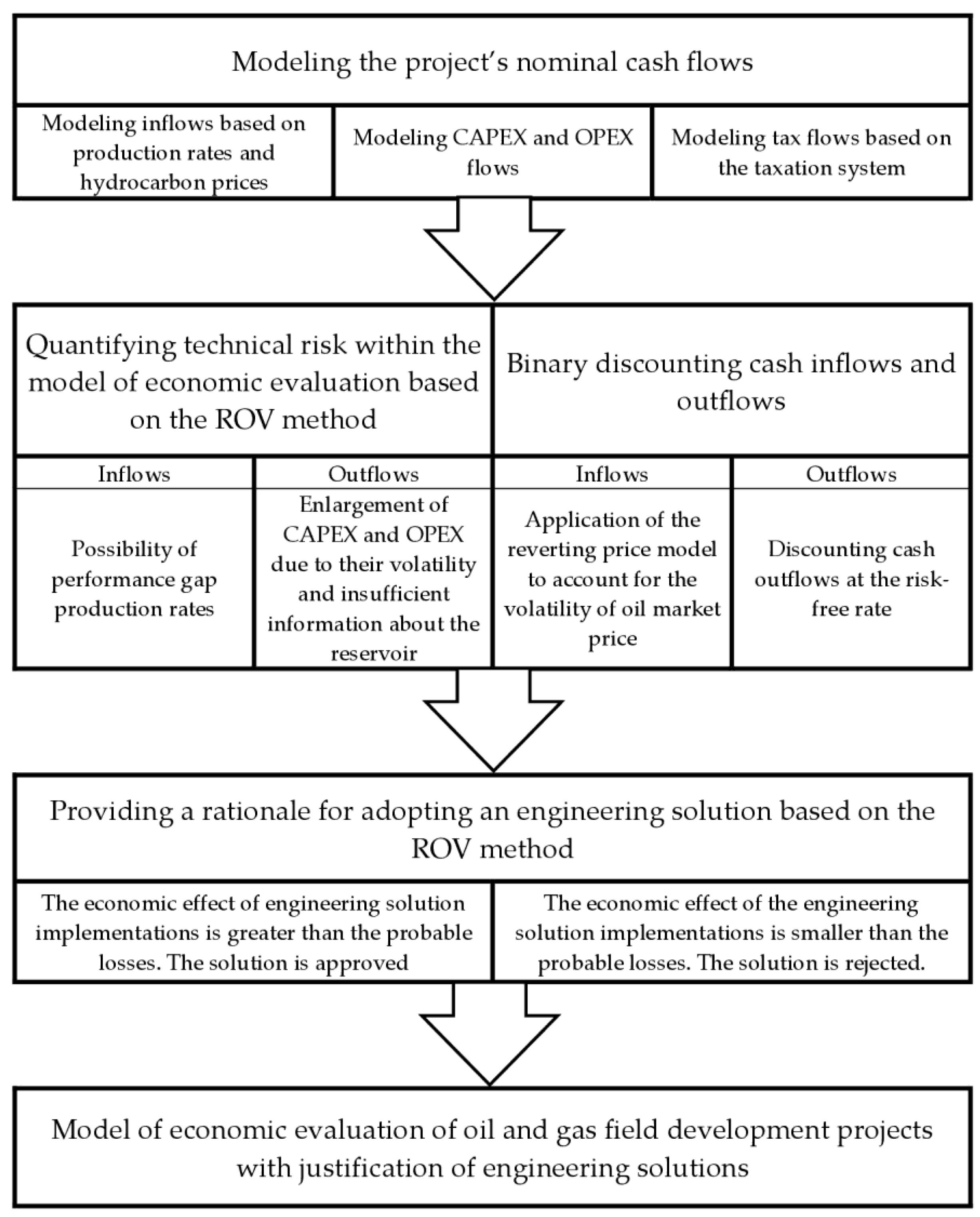
• Justification for each year of the forecast period of nominal values (excluding discounting) of cash inflows and outflows: revenue, operating costs, capital costs, taxes, etc.
• The use of binary discounting, i.e., separate discounting of inflows and outflows of the project at different rates. For inflows, the discount rate consists of two components: the risk-free rate (reflects the time factor) and the risk rate (reflects the change in the price of oil), which is calculated using a reverting price model. Outflows are discounted at a risk-free rate.
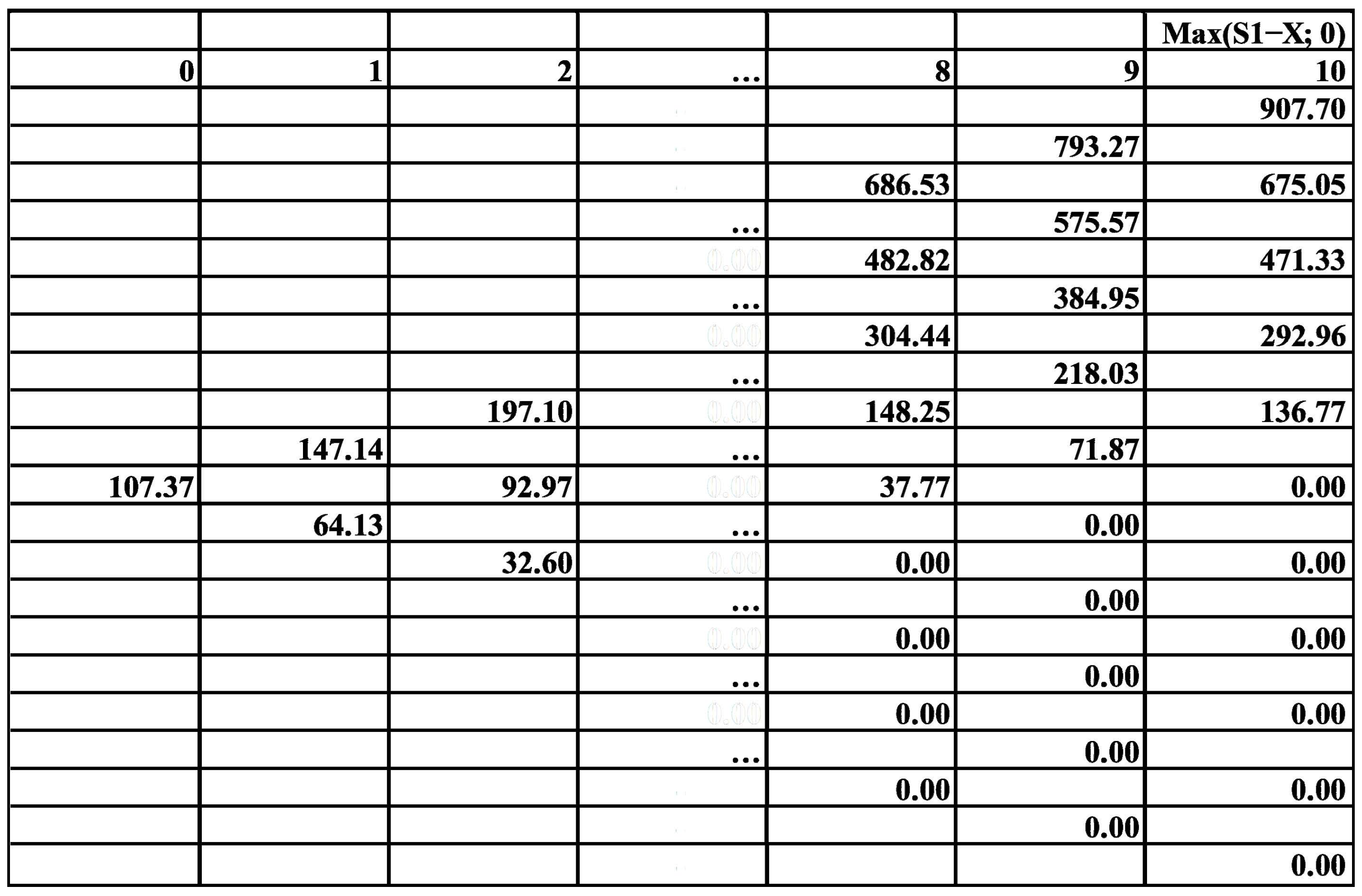
• Application of the real options valuation to calculate the absolute values of premiums for technical risks in the implementation of the project. For the inflows of each year of the project, the calculation of premiums is based on the projected change in production volumes. For outflows, capital expenditure premiums are calculated based on their volatility.
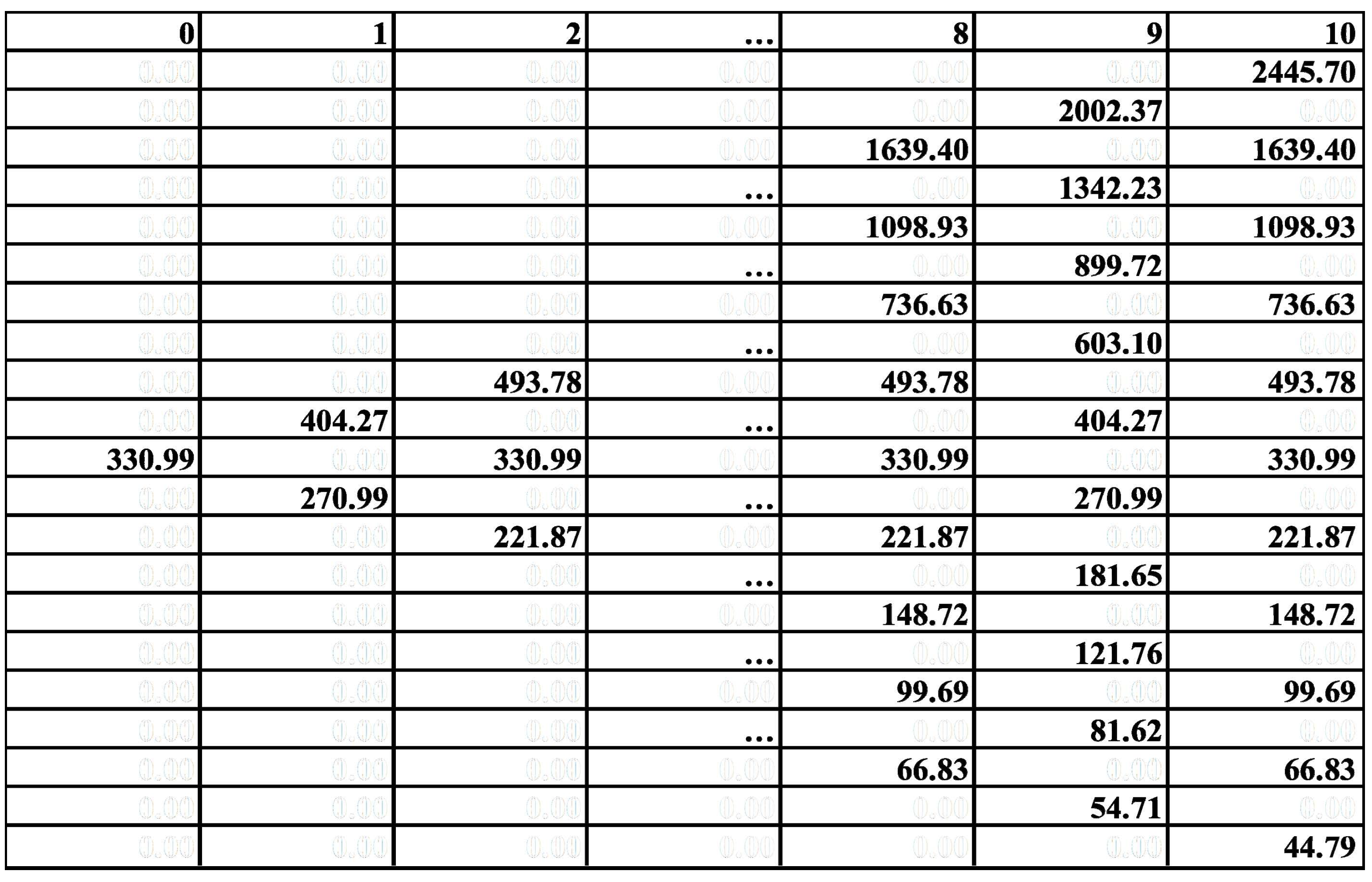
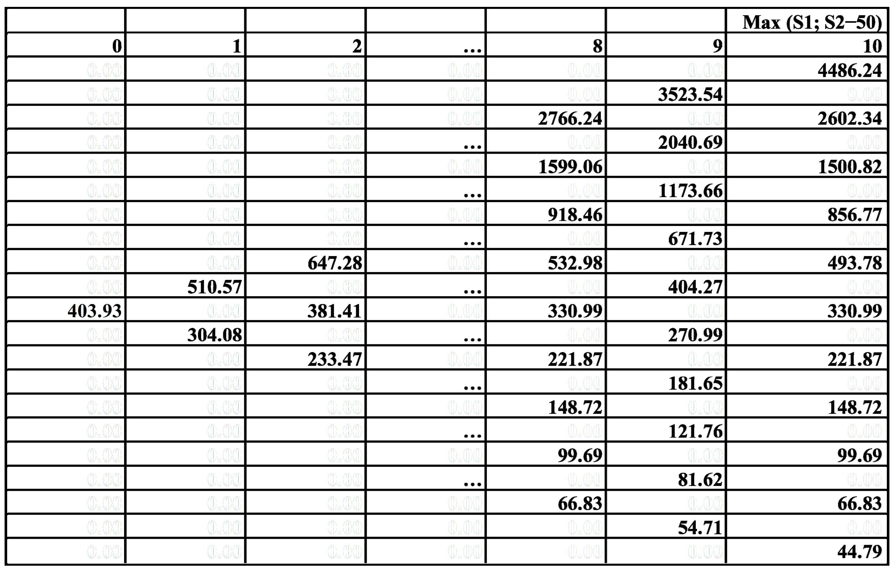
• The use of the real options valuation method to justify engineering decisions that can be made in the future of the project, from the available range of alternatives.

Further, these actions are considered in more detail.

2.1. Economic Evaluation of Oil and Gas Projects as Real Assets: Limitations of the DCF Method

Economic evaluation using the standard DCF method takes place in three steps. In the first step, the projected net cash flow is calculated for each period using the values of the determinants in the calculation model. In the second step, the net cash flows of the project are discounted using a certain rate (the rate of return or the discount rate). In the third step, the discounted value of the project’s cash flows is summed up. This approach leads to a reduction in future cash flows by a factor that grows exponentially over time by the same discount rate.

There are two approaches to finding the discount rate. The first approach is based on the value of the opportunity cost of capital (OCC), the weighted average cost of capital (WACC), or a similar indicator.

The second approach to determining the discount rate is to add the amount of project risk to the discount rate, i.e., to use a risk-adjusted rate. Any additional uncertainty not included in the cost of capital is offset by a yield premium, which is added to the rate. Therefore, the discount rate usually consists of two components: an expected risk-free rate and a risk rate. Within this framework, investors can calculate the discount rate using different methods:

• The capital asset pricing model (CAPM);
• Classifying projects by their basic parameters and assigning a different discount rate for each category (for example, one value for exploration projects, another for R&D projects, a third for development projects, etc.).

Regardless of how the rate of return is found, the traditional DCF method can be thought of as a top-down algorithm in which investors choose an appropriate discount rate, usually neglecting the specific features of individual projects. This is why no matter which of the two approaches is used, the model of economic evaluation will not change much. A significant problem in applying the DCF method to the valuation of real assets is project risks are assessed using economic and mathematical models covering a variety of net present values but not having any impact on the process of calculating the net present value.

Although providing certain decision-making criteria for all projects, the DCF method has a number of conceptual limitations [15]:

• It implies that the project is not changed, and the management follows the original plan regardless of changing circumstances without striving to eliminate uncertainties and increase the value of results;
• It assumes that future cash flows are predictable, which, as a rule, leads to the overestimation or underestimation of some types of projects;
• Insufficient consideration of the specific risks of the project, the need for adjustments increases the initial errors in the choice of the parameter and increases with the increase in the duration of the project.

The use of a single discount rate for the economic evaluation of an oil and gas project leads to a situation where an increase in the discount rate to account for market or non-systemic risk makes the impact of negative cash flows (for example, losses, expenses, unforeseen liabilities) that will arise in the distant future unreasonably insignificant. Additionally, regardless of the source of risk, risk factors are always represented by exponentially decreasing functions of time; hence, any error in estimating the discount rate will exponentially “fade” over time, which, for long-term mining projects, can lead to a significant accumulated error value [47]. Among other things, the application of a single rate causes a systematic error in the economic assessment process. This error can be proved using the principle of value additivity [59].

Summarizing the above, the biggest disadvantages of the DCF method associated with assuming the discount rate can be formulated as follows. The choice of the rate of return as a proxy for risk is largely arbitrary; the rate is chosen depending on investors’ preferences and experience [60,61]. Contradictory results (i.e., the higher the risk, the higher the NPV) can be obtained in cases where there is a cost-related risk. Once selected, the discount rate is assumed to be constant, even though the risk profile of the project usually changes over time, for instance, in relation to technical risk. The same rate of return applies to discounted assets (or liabilities) with different risk profiles. For high-risk projects (especially long-term ones) with a high rate of return, the DCF method greatly underestimates the impact of future cash flows [62].

2.2. Binary Model and Reverting Discounting for the Economic Evaluation of Oil and Gas Projects

For inflows and outflows of oil and gas projects, it is proposed to apply different discount rates [30], which are due to the change in rates over time of the project, taking into account the reduction in technical risks [40].

1. The proposed methodological approach assumes the use of distinct discount rates for variable determinants (revenue, royalties, operating costs, capital costs, capital cost allowance) and cash inflows and outflows of the project.

• It eliminated the systematic error that occurs when the single discount rate used by the company is applied to evaluate projects of different nature.
• Through discounting the individual determinants of the project, it removes the limitations that total cash flow discounting has.
• It combines risk and cost analyzes of a project by calculating the net present value of a project as the endpoint of all possible scenarios grouped together, as opposed to calculating the cost for each of the scenarios, and then by using this combination of costs in the economic evaluation process.

Mathematically, these limitations can be represented as follows. Present value of cash flow at time t is presented as:

PV_t = NCF_t/(1 + r)^t = NCF_t·1/(1+r)^t = NCF_t·DF_t,

(1)

where r is discount rate, which includes time and risk factors; DF_t is discount factor.

The discount factor (DF_t) for the cash flow of assets at time t could be presented as the ratio of the expected present value of cash flow to the most expected net cash flow:

DF_t = PV_t/NCF_t.

(2)

DF_t represents the proportionate decline in the value of the net cash flows of assets due to risk and time adjustments. Net cash flow is found as:

NCF_t = P_t·Q_t − OpEx_t − CapEx_t,

(3)

where NCF_t is the net cash flow in period t; P_t is the current expected selling price; Q_t is the volume of products sold; OpEx_t is operating expenditures; and CapEx_t is capital expenditures.

The same expression can be written as:

NCF_t = (P_t − UOpEx_t)·Q_t − CapEx_t,

(4)

where UOpEx_t is unit operating costs.

As mentioned earlier, the DCF method uses an aggregated risk and time adjustment approach that generates a DF_t for the cash flow at time t:

DF_DCFt = (((P_t − UOpEx_t)·Q_t − CapEx_t)·RiskDF_DCFt·TimeDF_t)/
/((P_t − UOpEx_t)·Q_t − CapEx_t),

(5)

where RiskDF_DCFt is the risk discount factor, which can be represented as e^{−Riskrate·t}; TimeDF_t is the time discount factor, which can be represented as e^{−Risklessrate·t}.

This expression can be simplified by reducing the net cash flow term as follows:

DF_DCFt = RiskDF_DCFt·TimeDF_t = e^{−Risk rate·t}·e^{−Risklessrate·t} = e^−RADR·t> 0

(6)

The equation shows that DF_DCF does not vary depending on the asset structure unless the RADR varies from asset to asset to reflect differences in asset risks, which is unlikely because many companies use the same RADR. However, it may not be possible to adequately adjust cash flows for risk, even using a RADR that tends to infinity. This becomes apparent once the DF_t is analyzed to discount the inflow and outflow determinants rather than the entire cash flow at once (DF_Det). Considering that the method under consideration adjusts the risk in the source of uncertainty (in this case, the price of hydrocarbons) and adjusts the time in the net cash flow, the following is true:

DF_Det = (((P_t·RiskDF_Det − UOpEx_t)·Q_t − CapEx_t)·TimeDF_t)/((P_t − UOpEx_t)·Q_t − CapEx_t)=
=TimeDF_t·(((F_t − UOpEx_t)·Q_t − CapEx_t)/((P_t − UOpEx_t)·Q_t − CapEx_t)),

(7)

where RiskDF_Det is the discount factor for price uncertainty in period t, which can be represented as e^{−Priceriskrate·t}; F_t is the forward price to period t.

This ratio cannot be simplified. The only case in which DF_Det = DF_DCF is when the elements of the cash flow are associated with equal risks. In most resource projects, the market risk in operating costs and capital costs is different, and there is usually less uncertainty in costs than in returns.

With a significant deviation from the discount curve in the standard DCF method, DCF DF_Det can become negative in situations where, for example, the forward price is less than unit operating costs, even though the expected cash flow on the asset may be positive. The standard DCF method does not produce a comparable result because the DF_DCF is always positive since the very risky cash flow with a positive expected value is capped at a non-negative risk-adjusted present value. Thus, there may be net cash flows whose risk-adjusted present value cannot be calculated using a positive DCF discount rate. A case in point is a risky net cash flow that has an expected value of zero. The standard DCF method will always calculate this net cash flow at a present value of zero [43].

2. The market uncertainty of hydrocarbon prices in the proposed approach is taken into account in the discount factor of inflows. Inflows are discounted by means of a reverting price model, which is proposed in [63], and its relevance for the oil and gas industry is confirmed in [64,65]. The reverting model implies that the greatest uncertainty and, consequently, risks associated with the volatility of hydrocarbon prices are inherent in the first periods. Consequently, the risk premium taken into account in the discount rate of inflows will decrease over time.

Being the product of risk-free rate and the cost of risk and the uncertainty of the forecast, the risk discount rate for inflows preserves the dependence of forecast uncertainty on the forecast period, and in this model, decreases for each year are added to the forecast period. The instant short-term rate is calculated [11] using the equation:

r = r_f + PRisk·σ,

(8)

where PRisk is the cost of risk arising from uncertainties in the hydrocarbon market [11]; σ is the uncertainty of the short-term forecast of the price of hydrocarbons.

To calculate the discount factor, the amount of uncertainty reduction with an increase in the planning horizon is taken into account [64], determined using the equation:

γ = ln(2)/HL,

(9)

where γ is the magnitude of the decrease in uncertainty with an increase in the planning horizon; HL is the length of time during which the uncertainty will decrease by half; in the current model, this is one year.

The time-varying discount factor for the price of hydrocarbons for the constant cost of risk is calculated by the equation:

DF_t = DF_f,t·e^{−PRiskσ/γ·(1 − s)},

(10)

where s = e^−γ·t; DF_f,t is risk-free discount factor; t is the year for which the factor is calculated. The ways in which the percolation effect, endogenous receipt of information from dynamic markets, and the influence of externalities affect information gathering incentives are described in more detail in the paper [66]. Treatment of the percolation in other branches of knowledge, for instance, in the study of network diffusion, is presented in the paper [67].

Costs are discounted at a risk-free rate. This moment can be attributed to the limitation of the model, since there is a risk of increased costs, which must be taken into account; in this regard, the discount rate for outflows should be less than risk-free, so that the deterministic values of outflows become larger, since they are adjusted for the amount of risk.

2.3. Application of the Theory of Real Options Valuation to Find the Cost of Risks of an Oil and Gas Development Project

The evaluation of oil and gas projects is associated with the growing uncertainty of their future profitability due to long life cycles. In addition to general market risks, oil and gas companies are influenced by geological and engineering risks. Therefore, investment projects for the development of oil and gas fields are assets that require the use of methods that account for the uncertainty factor as much as possible. Now, we will supplement the economic evaluation framework described above to account for technical uncertainties.

As previously noted, problems caused by using the DCF method can be avoided if the uncertainty associated with future cash flows and costs is decoupled from the time value of money, which will result in a more consistent project evaluation. As a rule, the biggest investment risks for any uncertain project are that the asset (i.e., cash inflow) may be worth less than expected and/or the cost of the asset (i.e., cash outflow) may be higher than expected. Instead of relying on investors’ risk preferences, an approach is proposed that combines risk assessment with the cost of risk. If we express the decrease in expected revenue and/or increase in expected expenditures in absolute terms, then the net present value equation can be written as follows:

NPV_t = ((CFR_r − S_CFRt) − (CFC_r + S_CFCt))/(1 + r)^t = ((CFR_t − CFC_t) − (S_CFRt + S_CFCt))/(1 + r)^t,

(11)

where NPV_t is the NPV of the project in period t, and the variables S_CFRt and S_CFCt are the expected fair values that represent the costs associated with the risk of income (i.e., asset value) falling below expected and that of costs exceeding the expected values, respectively, at some future moment t. As shown in Equation (11), these risk costs are accounted for separately and included in the analysis as extra project costs. Equation (11) can thus be written in a more general form as:

NPV_t = (CFR_t− CFC_t− S_t)/(1 + r)^t.

(12)

S_t = S_CFRt + S_CFCt represents the expected total cost of risk (in absolute terms) at time t as the sum of all risks that can be identified and considered.

Note that, unlike Equation (1), the discount rate r is risk-free. Thus, the factor of the time value of money is taken into account. The risk associated with the project is accounted for separately by the expected total cost of risk S_t. Factors of time and risk have been separated in Equation (13). It leads to their more correct accounting. In this regard, the higher the risk, the larger the value of S_t and, consequently, the lower the NPV value.In this form, the cost of risk actively encourages the company to analyze uncertainties associated with the geological and technical features of the project. The introduction of the concept of the absolute value of risk in Equation (12) reflects the acceptable amount of uncertainty for investors, i.e., the likelihood that revenue will be higher than expected and/or expenditures will be lower than expected. In other words, Equation (12)acquires the characteristics of an option and can be rewritten as(it is noted that Equation (12) simply represents the project’s NPV calculated using the risk-free rate minus the present value of the risk premium calculated in each period):

NPV_t (CFR_t; CFC_t; S_t; r) = NPV_t (CFR_t; CFC_t; r) − S_t/(1 + r)^t.

(13)

Volatility in the NPV of an oil and gas development project stems from:

• The influence of geological and technical conditions, which cause changes in the levels of production and costs;
• The situation in hydrocarbon production and transportation sectors;
• Market conditions in energy markets;
• The quality of the hydrocarbons produced at the given field;
• Local tax system, etc.

This is why projects for the development of hydrocarbon deposits can be classified as assets similar to options. The option characteristics of oil and gas projects produce uncertainties that arise during their implementation, which is mathematically expressed in Equation (13). To assess these characteristics, or the risks of the project, it is now possible to use the theory of real options, the methodological aspects of which are discussed in Appendix A.

The calculated risks components from Equation (13) in terms of the theory of real options can be expressed by applying the characteristics of put and call options. Put options (Equation (A2)) are used to account for uncertainties in the revenue stream, and call options (Equation (A1)) are used to account for uncertainties in the cost stream. The risk values calculated in this way are included in Equation (13), in the form of absolute, not relative values.

When using ROV methods, a question is how to determine volatility. This indicator should reflect both economic and technical uncertainties in the value of the underlying asset and how these uncertainties change over time. Some ROV experts argue that it is better to separate technical and market uncertainties, especially when decision making deals with technical uncertainty. In the discounting model presented above, the market risk is already represented by the reverse pricing model. Thus, only technical uncertainty will be determined.

Based on works by Dixit et al. and Espinoza et al. [49,68], technical volatility can be expressed as follows:

σ = ν·(α·β)^1/2,

(14)

where

α = (I/Q) = 1/T_c;

(15)

β ≅ (2 − T/T_c)/2;

(16)

ν = (2·v^2/(1 + v²))^1/2;

(17)

T_c is the expected completion time of the project; T is time to project completion; v is the time-independent factor of variation in flow cost estimated at t = 0.

The methodological approach to the evaluation of the oil and gas field development project, taking into account the engineering solution, is shown in Figure 1.

3. Results

Let us examine the possibility of deterministic estimation based on binary discounting and reverting discounting. A project for the development of some oil and gas condensate field (designated as A) is considered an asset subject to valuation. The basic version has the following production and cost parameters (

Table 1. Initial parameters.

Parameter	Value	Note
1. Development and production expenses, million RUB	962.87	In Year 0
2. Planning horizon, years	10	Starting from Year 1
3. Annual decrease in production, %	10	-
4. Initial production rate, million m3/year	254.52	-
5. Fixed operating expenditures, million RUB/year	119.16	0 in Year 0
6. Variable operating expenditures, RUB/m3	0.13	0 in Year 0

Source: Data on a conditional example of an oil and gas condensate field.

).

Fiscal conditions of the Russian Federation required for the calculation.

The income tax rate is 20%, the property tax is 2.2%, and the royalty is 1391 RUB/1000 m³. The price of the export netback of gas is conditionally assumed to be 4277 RUB/thousand m³. The price of gas is assumed to be the only source of market uncertainty in the cash flows of the project. Nominal cash flows and net present value of the project are calculated for r = 15% (

Table 2. Project evaluation by means of standard DCF, million RUB.

Parameter	0	1	2	3	4	…	7	8	9	10
Revenue		1 037.2	928.36	830.38	742.21	…	527.15	469.30	417.23	370.37
Operating expenditures		152.30	148.99	146.00	143.32	…	136.77	135.01	133.42	132.00
Capital expenditures	962.87					…
Depreciation		183.39	183.39	183.39	183.39	…	22.95	-	-	-
Taxes		371.19	331.75	295.85	263.14	…	188.15	169.33	152.40	137.16
Profit		330.34	264.23	205.14	152.36	…	179.28	164.96	131.41	101.21
Corporate tax		66.07	52.85	41.03	30.47	…	35.86	32.99	26.28	20.24
Net profit		264.27	211.39	164.11	121.89	…	143.42	131.96	105.13	80.97
Cash flow	−962.87	447.66	394.78	347.50	305.28	…	166.38	131.96	105.13	80.97
Discount factor	1.00	0.87	0.76	0.66	0.57	…	0.38	0.33	0.28	0.25
Discounted cash flow	−962.87	389.27	298.51	228.49	174.55	…	62.55	43.14	29.88	20.01
Accumulated discounted cash flow	−962.87	−573.60	−275.09	−46.60	127.94	…	409.62	452.76	482.64	502.65

Source: calculated by the authors.

).

At the next stage, the values of the discount rate for cash inflows and outflows of the project according to the binary model are justified. In Russian practice, a discount rate of 15% [1] is used, which is considered a risk-free rate plus a risk premium. As a risk-free rate for Russian conditions, the yield of 10-year bonds of the Russian Federation is used, the value of which at the valuation date, December 2020, is 6.14% (Bank of Russia. Russian Government Bond Zero Coupon Yield Curve, Values (% per annum). Available online: https://www.cbr.ru/hd_base/zcyc_params/?UniDbQuery.Posted=True&UniDbQuery.From=01.02.2019&UniDbQuery (accessed on 29 March 2022). Accordingly, the discount rate of 15% is considered as a risk-free rate (6.14%) plus a risk premium.

To forecast revenue, taking into account the influence of the price factor, the following assumptions are made. With short-term forecasts, there is uncertainty (σ) for oil price volatility of 27.28% per year (1.43% in daily terms). The values are calculated as the standard deviation of relative changes in oil prices over a 10-year period to 31 December 2020. The uncertainty of the forecast is halved for each subsequent year; accordingly, the uncertainty of the short-term forecast (σ) is calculated at the level of 0.273, and the cost of risk (PRisk) is assumed at the level of 0.3 [11].

A reverting model is used for discounting flows (Equations (8)–(10)); the values of discount rates (r) and discount coefficients (DF) are presented in

Table 3. Values of rates and discount factors for inflows.

T	0	1	2	3	4	5	6	7	8	9	10
DF	1.00	0.89	0.81	0.75	0.71	0.66	0.62	0.59	0.55	0.52	0.49
r, %	-	12.59	10.94	9.86	9.12	8.60	8.22	7.93	7.71	7.54	7.40

Source: calculated by the authors.

.

The economic evaluation and calculation of the NPV of the project were carried out using binary discounting and reversed discounting (

Table 4. Project evaluation by means of binary discounting and reverting discounting, million RUB.

Parameter	0	1	2	3	4	…	7	8	9	10
Revenue		921.20	754.23	626.29	523.53	…	308.96	259.03	216.92	181.39
Operating expenditures		143.49	132.25	122.10	112.92	…	90.12	83.82	78.04	72.74
Capital expenditures	962.87					…
Depreciation		172.78	162.79	153.37	144.50	…	15.13	0.00	0.00	0.00
Taxes		349.71	294.48	247.42	207.33	…	123.98	105.13	89.14	75.59
Profit		255.21	164.71	103.40	58.77	…	79.74	70.08	49.74	33.07
Corporate tax		51.04	32.94	20.68	11.75	…	15.95	14.02	9.95	6.61
Net profit		204.17	131.77	82.72	47.02	…	63.79	56.07	39.79	26.46
Cash flow	−962.87	376.95	294.56	236.09	191.52	…	78.91	56.07	39.79	26.46
Discount factor	1	1	1	1	1	…	1	1	1	1
Discounted cash flow	−962.87	376.95	294.56	236.09	191.52	…	78.91	56.07	39.79	26.46
Accumulated discounted cash flow	−962.87	−585.92	−291.36	−55.27	136.25	…	474.22	530.29	570.08	596.53

Source: Calculated by the authors.

), the project revenue was discounted at rates (Table 3), and costs were discounted at a risk-free rate of 6.14%.

Table 5. Comparison of NPV magnitudes for a project with different calculation methods.

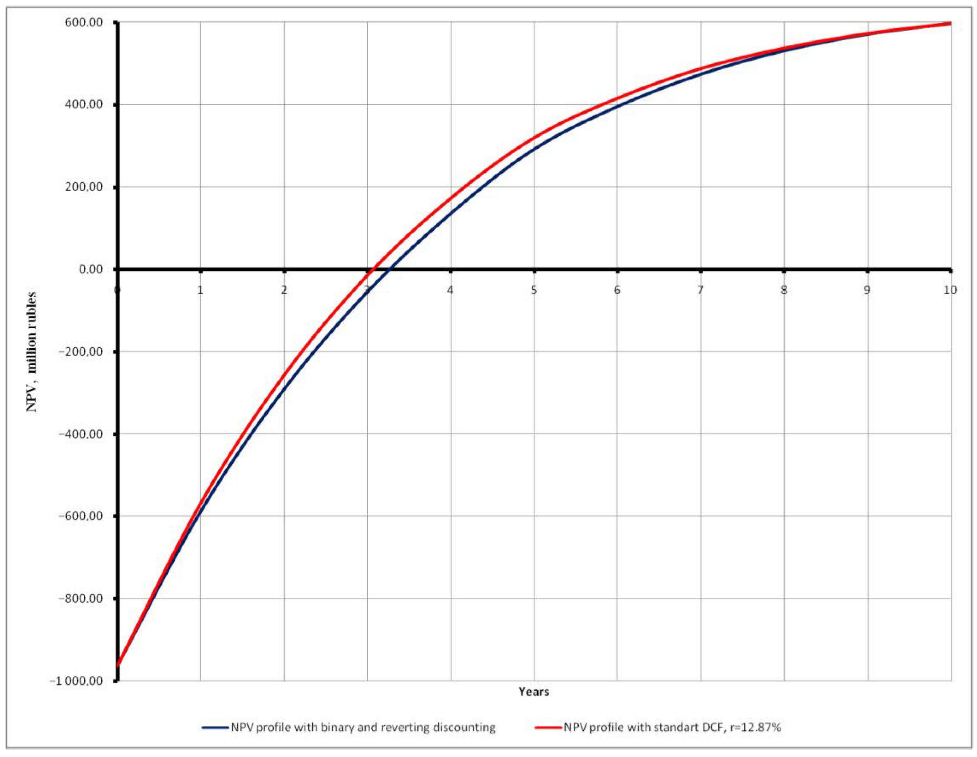
Standard DCF
Discount rate, %	15
NPV, million RUB	502.65
Reverting and binary discounting
Discount rate,%	12.87
NPV, million RUB	596.53

Source: Calculated by the authors.

shows the NPV magnitudes for the oil and gas field development project and their comparison for various calculation methods.

Figure 2 shows graphs of changes in the NPV of the project calculated at different rates. The bottom graph shows the dynamics of net present value with binary discounting of revenue at the rates of the reverting model (Table 3) and costs at the risk-free rate of 6.14%; the upper graph reflects the change in cash flow obtained using the classical DCF method with a discount rate of 12.87%. The NPVs are the same and equal to RUB 596.53 million. The graph corresponding to the classical calculation shows that the NPV build-up in the first few years is faster, and the later flows have a lower specific gravity compared to the second method. This confirms that the traditional discounting model downplays late cash flows and exaggerates early ones. This is one of the reasons why operating companies often intensify production, since the evaluation model shows that it is possible to make a big profit by extracting (and then selling) fluids as quickly as possible, rather than adhering to a systematic progressive development that implies producing as many resources as possible. The modified method means ‘softer’ discounting and equally distributed reduction in the future value. The classic DCF method underestimates projects with a long implementation horizon, while overestimating projects with extraordinary cash flows.

Next, an economic valuation of the technical risk of the development of a hydrocarbon deposit is carried out using the theory of real options. As uncertainties, the values of debits and the variability of capital expenditures are considered.

Table 6. Risk costs in the implementation of technical risk (drop in debits).

T, Period	0	1	2	3	4	5	6	7	8	9	10
σ (Equation (14))	20.0%	19.5%	19.0%	18.4%	17.9%	17.3%	16.7%	16.1%	15.5%	14.8%	14.1%
Risk component (Equation (A2)), million RUB	-	51.65	44.46	38.14	32.60	27.74	23.49	19.78	16.55	13.73	11.28
d1 (Equation (A3))	-	0.41	0.41	0.42	0.42	0.43	0.44	0.45	0.46	0.48	0.49
d2 (Equation (A4))	-	0.21	0.22	0.23	0.25	0.26	0.27	0.29	0.31	0.33	0.35

Source: calculated by the authors.

shows the calculation of the risk values for the revenue stream (put option, Equation (A2) of the Appendix A). At the same time, the coefficient of variation V of the flow rate array of appraisal wells is determined to be 0.5, the term of the option, T = 1 year, since it is calculated annually, the duration of the project has not changed for 10 years. Equations for calculations are presented in the Appendix A.

The capital expenditures of the project are RUB 962.87 million. This estimated value is for a year before starting production, so it may change. The company’s analysts, based on similar implemented projects and internal methods of the company, calculated the coefficient of variation for capital investments, V = 0.15. The premium for the technical risk of volatility of capital expenditures is equal to the value of the call option (Equation (13)), where S1 is the current value of the underlying asset, the values of which are presented in the extreme column in Figure 3; X is the strike price equal to the value of the initial capital costs.

Volatility is calculated for the next year (Equations (14)–(17), T_c = 1 years; T = 0 years) and will be 21%. A binomial lattice is used to calculate the call option, as the flow of costs is estimated. Binomial lattice parameters: u = 1.069, ΔT = 0.1, d = 0.936, r_f = 6% (yield of one-year, not ten-year, government bond), p = 0.53. The grid of the underlying asset and the evaluation grid are shown in Figure 3 and Figure 4.

The cost of the call option, i.e., the cost of the capital cost risk associated with the change in debits, amounted to RUB 107.37 million.

Table 7. NPV of the project taking into account the cost of price and technical risks.

Parameter	0	1	2	3	4	…	7	8	9	10
Revenue		1037.2	928.36	830.38	742.21	…	527.15	469.30	417.23	370.37
Revenue minus risk component (Table 6)		985.57	883.90	792.24	709.61	…	507.37	452.75	403.50	359.09
Discounted risk-free revenue (based on Table 3)		875.83	718.52	597.86	500.81	…	297.53	250.02	209.88	175.96
Operating expenditures		143.49	132.25	122.10	112.92	…	90.12	83.82	78.04	72.74
Capital expenditures (factoring in the risk component)	1070.27					…
Depreciation		172.78	162.79	153.37	144.50	…	15.13	0.00	0.00	0.00
Taxes		349.71	294.48	247.42	207.33	…	123.98	105.13	89.14	75.59
Profit		209.84	129.00	74,97	36.06	…	68.30	61.08	42.70	27.63
Net profit		167.87	103.20	59,98	28.85	…	54.64	48.86	34.16	22.10
Cash flow	−1070.2	340.66	265.99	213,35	173.35	…	69.76	48.86	34.16	22.10
Discount factor	1	1	1	1	1	…	1	1	1	1
Discounted cash flow	−1070.2	340.66	265.99	213,35	173.35	…	69.76	48.86	34.16	22.10
Accumulated discounted cash flow	−1070.2	−729.58	−463.59	−250,25	−76.90	…	225.85	274.72	308.88	330.99

Source: calculated by the authors.

presents an economic assessment of the oil and gas field development project at net present value, taking into account the values of risk values obtained. The cost of risk is deducted from the revenue in case of a possible drop in debits, and then the flow is discounted with coefficients according to the reversed model. Capital expenditures increased by a risk premium of RUB 107.37 million (Figure 4); then, outflows are discounted at a risk-free rate.

At the final stage, an economic evaluation of engineering solutions for the development of oil and gas fields using ROV is carried out.

An example of an engineering solution is the expansion of the array of producing wells in the 0th year of the project. The oil and gas company has two development options.

Option 1. The rejection of this engineering solution gives an NPV of RUB 330.99 million. The coefficient of variation V of the flow rate array of appraisal wells is determined to be 0.5, so the volatility in the zeroth year is 20%.

Option 2, the expansion of the production system, gives an NPV of RUB 310 million, excluding capital costs for drilling (X), RUB 50 million. When implementing this option, the fund of producing wells increases, which, accordingly, increases the coefficient of variation V of the array of well flow rates. The coefficient of variation is assumed to be 0.75, so the volatility is 26.83% (Equations (14)–(17)).

Calculations are presented in

Table 8. Parameters for evaluating an engineering solution for expanding the array of wells using the real options method.

Parameter	Option 1	Option 2
Volatility, σ	0.2	0.27
ΔT, years	1	1
u	1.22	1.31
d	0.818	0.765
rf	6.14%	6.14%
X, million RUB	-	50 (costs associated with the engineering solution)
NPV, million RUB	330.99	310 (without factoring in 50 m for drilling)

Source: compiled by the authors.

.

Option 2 with the expansion of the array of wells creates new opportunities for extracting more hydrocarbons. However, it also means a bigger probability of an increase in oil–water ratio, which, in turn, means a bigger volatility σ. In addition, the final NPV is affected by the physical, chemical, and geological conditions of the reservoir, of which more will be known in a year, when it is planned to introduce the solution. The decision is made here and now, and it is preferable to choose Option 1.

We interpret the engineering solution as an option. Then, the capital cost of drilling is the exercise price of the option. To carry out the analysis using the ROV method, two grids of the underlying asset are constructed (Figure 5 and Figure 6) with an estimate of the array of probable values of the net value of the asset, when it is estimated for 10 years of project implementation using traditional DCF.

Let us interpret the engineering solution as an option. Then, drilling costs are the strike price of the option. To use the ROV method, two underlying asset lattices are made (Figure 5 and Figure 6) with an assessment of the array of probable values of the net asset value, as if the asset was assessed in Year 10 using the standard method.

For Option 2, the boundary condition is used. Drilling costs are subtracted from the expected distributed NPV (RUB 50 million; all other cash flows that emerge after the implementation of the solution are taken into account in the model and affect the NPV array). It is assumed that in 10 years, the company will choose the best of the nodes of the net asset value. If the global events and the inherent risks correspond to the values in the upper nodes (the most positive ones), then the option with an engineering solution will become more valuable than without it. Additionally, if the company preferred Option 1 in Year 0, it means it missed out on the value added by the engineering solution. Additionally, if the conditions follow the path of the lower bound, then Option 1 will still be preferable in ten years’ time.

To find the possible value added by an engineering solution, it is necessary to complete the assessment by making a valuation lattice (Figure 7). For each node, the maximum of the two possible values is selected.

Using the ROV method showed that the probable value added by the decision to expand on drilling is RUB 72.94 million (403.93 million minus 330.99 million). This is the added value of the project that can be created by an engineering solution. Probable losses amount to RUB 70.99 million (330.99 minus 310 with 50 for drilling). Having compared the probable value added and the probable losses, the company will decide to implement an engineering solution, i.e., choose Option 2.

4. Discussion

The paper proposes a methodological approach to the economic evaluation and justification of engineering solutions in the implementation of oil and gas field development projects, developed on the basis of a comprehensive application of binary discounting methods, reverting discounting based on the DNPV method using the theory of real options.

The developed methodological approach makes it possible to determine the probable net added value of the project when making an engineering decision, allowing avoiding the bias of the financial model for evaluating real projects.

The increase in the added value of the project can be provided by taking into account the following factors:

• Optimization of the reservoir model at the design phase with the emergence of new opportunities to respond to technological and geological challenges through engineering solutions;
• Rationalization of the field development system during production by improving reservoir parameters through engineering solutions, covering a larger area, or improving fluid movement in the reservoir, thereby reducing technical uncertainties and creating prerequisites for increasing the recovery factor;
• Taking into account changes in macroeconomic indicators, in particular, the situation of global energy markets.

Using the proposed methodological approach to validate the adoption of engineering solutions, companies will align their actual and planned performance indicators. Deviations of indicators associated with insufficient geological knowledge of the object, an unsuccessfully chosen field development system, necessitates changes, adjustments to design documents, geological and hydrodynamic models, and the choice of measures to regulate the development of an operational object. This is where evaluation and substantiation of engineering solutions need to be an integral part of the process.

The optimization of the engineering solution can improve the parameters of the hydrocarbon production process, reduce technical uncertainties, and improve the financial performance indicators of oil and gas projects (in addition, the adoption of certain engineering decisions (for example, drilling injection wells) during the development of oil and gas fields may indirectly affect factors including a social significance factor such as groundwater resources management [69]). It is important to note that this does not depend on some external factors, such as oil prices or the productive capacity of the reservoir, which the oil and gas company cannot change, but on the company itself.

5. Conclusions

The standard DCF model for the economic evaluation of oil and gas projects has conceptual limitations, such as static character, deterministic character of future cash flows, and insufficient consideration of specific project risks. In addition, the use of a single discount rate has the following disadvantages: the rate is chosen depending on the preferences of investors, the inconsistency of the results for discounting negative flows, the rate is considered constant, and for long-term projects, the contribution of future cash flows is significantly minimized. These limitations lead to distortion of the economic assessment of the investment project, including subsequent engineering decisions.

In order to eliminate the biases of the DCF method of economic evaluation of oil and gas projects with engineering solutions, it is proposed to apply models of binary discounting, reverting pricing and the real options valuation. The use of binary discounting makes it possible to eliminate the disadvantages of applying a single rate of return. The reverting pricing model takes into account market risks when evaluating an oil and gas field development project. The discount rate for inflows becomes dynamically variable. In the first year of the project, it has the largest value, and then it decreases for each subsequent period, which reflects the peculiarities of oil price volatility.

The use of the real options valuation makes it possible to calculate absolute premiums for investment risks that arise due to the variability of capital expenditures and for technical risks, which are produced by possible decreases in production well rates. The theory of real options is also used to determine the added value of an engineering solution that arises during the implementation of a project.

The considered tools are implemented in the developed methodological approach to the economic evaluation of oil and gas projects and the justification of engineering solutions. The proposed approach has been tested on a conditional example of an oil and gas field development project. The application of the approach justified the adoption of an engineering decision to expand the grid of producing wells. Such a decision at the initial analysis had a negative economic effect within the framework of the project.

The main contribution and scientific novelty of the manuscript are:

• The methodological approach to substantiating various discount rates for inflows and outflows during the development of oil and gas fields makes it possible to more realistically take into account the specifics of oil and gas fields development projects, including both long terms and the requirement to intensify production through the use engineering solutions and oil price volatility.
• The implementation of a combination of binary discounting and reverting discounting. By itself, binary discounting allows us to correctly take into account, first of all, the risks of outflows, and reverting discounting—the risks of inflows. Thus, the discount model, which is elaborated due to their combination, enables us to correctly take into account the risks of both types.
• Reasonable choice of the discount rate for inflows, taking into account the reduction in oil price volatility, enables us to obtain more correct values of discounted inflows and improve the economic efficiency of the oil and gas fields’ development project.
• Reasonable choice of the discount rate for outflows, taking into account the absolute magnitudes of risks, including investment flows of engineering solutions produced over a number of years, allows us to obtain more correct values of discounted outflows and make more valid conclusions about the economic efficiency of the oil and gas fields’ development project, including the reduction in economic efficiency.

The methodological approach proposed by the authors assumes consideration of price, technical, mining, and geological risks. The main limitations of the study are:

• The reduction in oil price volatility in the long term is estimated using a logarithmic model. This is an assumption that may not correspond to real conditions in the global market. In modern conditions, in addition to economic factors, the situation on the oil market is influenced by the ESG agenda. That is, the model can be refined and expanded because of the new factors.
• The sensitivity analysis of the results obtained has not been performed, taking into account the structure of cash flows in the financial model for various oil and gas fields: the ratio between inflows and outflows by year, the distribution of cash flows by year, the non-negativity of cash flows by year, the composition of inflows and outflows, the marginality of products, and the composition of taxes.
• The calculation was made for one case. Therefore, it is necessary to continue the economic evaluation of deposits with various types and sizes, with different investment structures and under different tax conditions.
• There is incomplete accounting of the spectrum of risks accompanying the implementation of oil and gas projects.

The authors consider further promising research in the following areas: a deeper study of the relationship between various types of oil and gas project risks that may be influenced by engineering decisions to include them in the economic evaluation model; a study of the impact of the uncertainties identified in the article on the financial performance of oil and gas development projects; classification of engineering solutions in terms of their impact on the change in flow rates, capital and operating expenditures, and cash flows in oil and gas projects.

The authors are not aware of cases of practical implications of this methodological approach in the economic evaluation and justification of engineering solutions in the implementation of projects for the development of oil and gas fields. The authors see the prospect of this approach for evaluating not only oil and gas projects, but also mineral production projects and construction and agricultural projects, i.e., projects with a long implementation period and/or high volatility of prices for the final product.

References

- Ministry of Natural Resources and Environment of the Russian Federation. Rules on the Preparation of Technical Projects for the Development of Hydrocarbon Deposits; Ministry of Natural Resources and Environment: Moscow, Russia, 2019. [Google Scholar]
- Ministry of Natural Resources and Environment of the Russian Federation. Rules on the Development of Hydrocarbon Deposits; Ministry of Natural Resources and Environment: Moscow, Russia, 2016. [Google Scholar]
- Clews, R.J. Project Finance for the International Petroleum Industry, 1st ed.; Elsevier Inc.: Amsterdam, The Netherlands, 2016. [Google Scholar]
- Fermi, D.W.; Yusri, B.A.; Haeryip, S. Monte Carlo net present value for techno-economic analysis of oil and gas production sharing contract. Int. J. Technol. 2019, 10, 829–840. [Google Scholar]
- Jafarizadeh, B.; Bratvold, R.B. Project Economics in the Big-Bets Industry: The Integrated Valuation in Practice. J. Pet. Sci. Eng. 2021, 197, 108095. [Google Scholar] [CrossRef]
- Berntsen, M.; Bøe, K.S.; Jordal, T.; Molnár, P. Determinants of oil and gas investments on the Norwegian Continental Shelf. Energy 2018, 148, 904–914. [Google Scholar] [CrossRef]
- Kh, M.R. Nefteotdacha: Proshloe, Nastoyashchee, Budushchee (Optimizatsiya Dobychi, Maksimizatsiya KIN) (Oil Recovery: Past, Present, Future (Production Optimization, Maximization of Recovery Factor)); Kazan’: FEN Publishing House: Kazan, Russia, 2014; p. 750. [Google Scholar]
- Muslimov, R.K. History and prospects of hydrodynamic methods for oil fields development in Russia. Neftyanoe Khozyaystvo—Oil Ind. 2020, 12, 95–100. [Google Scholar] [CrossRef]
- Tang, B.-J.; Zhou, H.-L.; Chen, H.; Wang, K.; Cao, H. Investment opportunity in China’s overseas oil project: An empirical analysis based on real option approach. Energy Policy 2017, 105, 17–26. [Google Scholar] [CrossRef]
- Jafarizadeh, B.; Bratvold, R.B. Sequential Exploration: Valuation with Geological Dependencies and Uncertain Oil Prices. SPE J. 2020, 25, 2401–2417. [Google Scholar] [CrossRef]
- Salahor, G. Implications of output price risk and operating leverage for the evaluation of petroleum development projects. Energy J. 1998, 19, 13–46. [Google Scholar] [CrossRef]
- Yakupov, R.F.; Mukhametshin, V.S.; Khakimzyanov, I.N.; Trofimov, V.E. Optimization of reserve production from water oil zones of D3ps horizon of Shkapovsky oil field by means of horizontal wells. Georesursy 2019, 21, 55–61. [Google Scholar] [CrossRef]
- Muslimov, R.K. Fundamental problems of oil industry. Neftyanoe Khozyaystvo—Oil Ind. 2017, 1, 6–11. [Google Scholar]
- Adkins, R.; Paxson, D. Rescaling-contraction with a lower cost technology when revenue declines. Eur. J. Oper. Res. 2019, 277, 574–586. [Google Scholar] [CrossRef]
- Bailey, W.; Couët, B.; Bhandari, A.; Faiz, S.; Srinivasan, S.; Weeds, H. Unlocking the value of real options. Oilfield Rev. 2003, 15, 4–19. [Google Scholar]
- Bera, A.; Kumar, T.; Ojha, K.; Mandal, A. Adsorption of surfactants on sand surface in enhanced oil recovery: Isotherms, kinetics and thermodynamic studies. Appl. Surf. Sci. 2013, 284, 87–99. [Google Scholar] [CrossRef]
- Sedaghata, M.H.; Mohammadib, H.; Razmia, R. Application of SiO2 and TiO2 nanoparticles to enhance the efficiency of polymer-surfactant floods. Energy Sources Part A Recovery Util. Environ. Eff. 2016, 38, 22–28. [Google Scholar] [CrossRef]
- Rogachev, M.K.; Aleksandrov, A.N. Justification of a comprehensive technology for preventing the formation of asphalt-resin-paraffin deposits during the production of highly paraffinic oil by electric submersible pumps from multiformation deposits. J. Min. Inst. 2021, 250, 596–605. [Google Scholar] [CrossRef]
- Dvoynikov, M.V. Designing of well trajectory for efficient drilling by rotary controlled systems. J. Min. Inst. 2018, 231, 254–262. [Google Scholar]
- Wang, K.; Vredenburg, H.; Wang, T.; Feng, L. Financial return and energy return on investment analysis of oil sands, shale oil and shale gas operations. J. Clean. Prod. 2019, 223, 826–836. [Google Scholar] [CrossRef]
- Sharpe, W.F. Capital asset prices: A theory of market equilibrium under conditions of risk. J. Financ. 1964, 19, 425–442. [Google Scholar]
- Myers, S.C.; Turnbull, S.M. Capital budgeting and the capital asset pricing model: Good news and bad news. J. Financ. 1977, 32, 321–333. [Google Scholar] [CrossRef]
- Rogachev, M.K.; Mukhametshin, V.V.; Kuleshova, L.S. Improving the efficiency of using resource base of liquid hydrocarbons in jurassic deposits of western Siberia. J. Min. Inst. 2019, 240, 711–715. [Google Scholar] [CrossRef] [Green Version]
- Rogachev, M.K.; Mukhametshin, V.V. Control and regulation of the hydrochloric acid treatment of the bottomhole zone based on field-geological data. J. Min. Inst. 2018, 231, 275–280. [Google Scholar]
- Dvoinikov, M.V.; Kuchin, V.N.; Mintsaev, M.S. Development of viscoelastic systems and technologies for isolating water-bearing horizons with abnormal formation pressures during oil and gas wells drilling. J. Min. Inst. 2021, 247, 57–65. [Google Scholar] [CrossRef]
- Hawas, F.; Cifuentes, A. Valuation of projects with minimum revenue guarantees: A Gaussian copula-based simulation approach. Eng. Econ. 2017, 62, 90–102. [Google Scholar] [CrossRef]
- Shkatov, M.Y.; Sergeev, I.B. The evaluation of cost efficiency of mineral exploration and mining investment projects: Development of the income approach. Mineral Resources of Russia. Econ. Manag. 2007, 1, 38–44. [Google Scholar]
- Fama, E. Risk-adjusted discount rates and capital budgeting under uncertainty. J. Financ. Econ. 1977, 5, 3–24. [Google Scholar] [CrossRef]
- Philbrick, S.W. Accounting for risk margins. Casualty Actuar. Soc. Spring Forum 1994, 1, 1–87. [Google Scholar]
- Robichek, A.A.; Myers, S.C. Conceptual problems in the use of risk-adjusted discount rates. J. Financ. 1966, 21, 727–730. [Google Scholar]
- Viscusi, W.K. Rational discounting for regulatory analysis. Univ. Chic. Law Rev. 2007, 74, 209–246. [Google Scholar]
- Gert, A.A.; Suprunchik, N.A.; Nemova, O.G.; Kuzmina, K.N. Valuation of Oil and Gas Fields and Subsoil Plots, 2nd ed.; OOO Geoinformmark: Moscow, Russia, 2010; ISBN 978-5-98877-038-1. [Google Scholar]
- Gert, A.A.; Volkova, K.N.; Nemova, O.G.; Suprunchik, N.A. Methods and Practical Experience of Valuation of Oil and Gas Reserves and Resources; Science: Novosibirsk, Russia, 2007; ISBN 5-02-032557-0. [Google Scholar]
- Tugan, M.F.; Sinayuc, C. A new fully probabilistic methodology and a software for assessing uncertainties and managing risks in shale gas projects at any maturity stage. J. Pet. Sci. Eng. 2018, 168, 107–118. [Google Scholar] [CrossRef]
- Cherepovitsyn, A.; Metkin, D.; Gladilin, A. An algorithm of management decision-making regarding the feasibility of investing in geological studies of forecasted hydrocarbon resources. Resources 2018, 7, 47. [Google Scholar] [CrossRef] [Green Version]
- Zhu, L.; Zhang, Z.X.; Fan, Y. Overseas oil investment projects under uncertainty: How to make informed decisions? J. Policy Model. 2015, 37, 742–762. [Google Scholar] [CrossRef]
- Marinina, O.A. Classification and methods of the accounting of investment risks of oil and gas projects. J. Min. Inst. 2013, 205, 202–207. [Google Scholar]
- Laughton, D.G. The potential for use of modern asset pricing methods for upstream petroleum project evaluation: Introductory remarks. Energy J. 1998, 19, 1–11. [Google Scholar] [CrossRef]
- Bradley, P.G. On the use of modern asset pricing for comparing alternative royalty systems for petroleum development projects. Energy J. 1998, 19, 47–81. [Google Scholar] [CrossRef]
- Laughton, D. The management of flexibility in the upstream petroleum industry. Energy J. 1998, 19, 83–114. [Google Scholar] [CrossRef]
- Baker, M.P.; Scott Mayfield, E.; Parsons, J.E. Alternative models of uncertain commodity prices for use with modern asset pricing methods. Energy J. 1998, 19, 115–148. [Google Scholar] [CrossRef] [Green Version]
- Laughton, D.G.; Sagi, J.S.; Samis, M.R. Modern asset pricing and project evaluation in the energy industry. West. Cent. Econ. Res. 2000, 56, 3–46. [Google Scholar]
- Samis, M.; Davis, G.A.; Laughton, D.; Poulin, R. Valuing uncertain asset cash flows when there are no options: A real options approach. Resour. Policy 2006, 30, 285–298. [Google Scholar] [CrossRef]
- Guj, P.; Garzon, R. Modern Asset Pricing—A Valuable Real Option Complement to Discounted Cash Flow Modeling of Mining Projects. In Proceedings of the Project Valuation Conference, Melbourne, Australia, 19–20 April 2007. [Google Scholar]
- Espinoza, R.D.; Morris, J.W.F. Decoupled NPV: A simple, improved method to value infrastructure investments. Constr. Manag. Econ. 2013, 31, 471–496. [Google Scholar] [CrossRef]
- Espinoza, R.D. Decoupling time value of money and risk: A step toward the integration of risk management and quantification. Int. J. Proj. Manag. 2014, 32, 1056–1072. [Google Scholar] [CrossRef]
- Espinoza, R.D.; Rojo, J. Towards sustainable mining (Part I): Valuing investment opportunities in the mining sector. Resour. Policy 2017, 52, 7–18. [Google Scholar] [CrossRef]
- Pindyck, R. Investments of uncertain cost. J. Financ. Econ. 1993, 34, 53–76. [Google Scholar] [CrossRef] [Green Version]
- Espinoza, R.D. Contingency estimating using option theory: Closing the gap between theory and practice. Constr. Manag. Econ. J. 2011, 29, 913–927. [Google Scholar] [CrossRef]
- Armstrong, M.; Galli, A.; Bailey, W.; Couët, B. Incorporating technical uncertainty in real option valuation of oil projects. J. Pet. Sci. Eng. 2004, 44, 67–82. [Google Scholar] [CrossRef]
- Ponomarenko, T.V.; Sergeev, I.B. Valuation of mineral assets of a mining company on the basis of the option approach. J. Min. Inst. 2011, 191, 164–175. [Google Scholar]
- Galevsky, S.G. A binary model of discounting cash flows to correct risk assessment for real assets evaluation. Tomsk. State Univ. J. Econ. 2020, 49, 122–140. [Google Scholar] [CrossRef] [PubMed]
- Myers, S.C. Determinants of corporate borrowing. J. Financ. Econ. 1977, 5, 147–176. [Google Scholar] [CrossRef] [Green Version]
- Myers, S.C. Finance theory and financial strategy. Interfaces 1984, 14, 126–137. [Google Scholar] [CrossRef]
- Davis, G.A.; Samis, M. Using Real Options to Value and Manage Exploration. In Wealth Creation in the Minerals Industry: Integrating Science, Business, and Education; Doggett, M.D., Parry, J.R., Eds.; Society of Economic Geologists: Easton, MD, USA, 2006; pp. 273–294. [Google Scholar]
- Shafiee, S.; Topal, E.; Nehring, M. Adjusted real option valuation to maximise mining project value—A case study using century mine. Australas. Inst. Min. Metall. Publ. Ser. 2009, 3, 125–134. [Google Scholar]
- Kruk, M.N.; Nikulina, A.Y. Economic estimation of project risks when exploring sea gas and oil deposits in the Russian arctic. Int. J. Econ. Financ. Issues 2016, 6, 138–150. [Google Scholar]
- Damodaran, A. Investment Valuation: Tools and Techniques for Determining the Value of Any Asset, 2nd ed.; Wiley: Oxford, UK, 2002. [Google Scholar]
- Miller, M.H.; Modigliani, F. Dividend Policy, Growth and the Valuation of Shares. J. Bus. 1961, 34, 411–433. [Google Scholar] [CrossRef]
- Arnold, G.; Hatzopoulos, P.D. The theory practice gap in capital budgeting: Evidence from the United Kingdom. J. Bus. Financ. Account. 2000, 27, 603–626. [Google Scholar] [CrossRef]
- Davies, R.; Goedhart, M.; Koller, T. Avoiding a risk premium that unnecessarily kills your project. McKinsey Q. 2012, 2, 1–4. [Google Scholar]
- Gollier, C. Time horizon and the discount rate. J. Econ. Theory 2002, 107, 463–473. [Google Scholar] [CrossRef] [Green Version]
- Laughton, D.G.; Jacoby, H.D. Reversion, Timing Options, and Long-Term Decision-Making. Financ. Manag. 1993, 22, 225–240. [Google Scholar] [CrossRef]
- Schwartz, E.S. The stochastic behavior of commodity prices: Implications for valuation and hedging. J. Financ. 1997, 52, 923–973. [Google Scholar] [CrossRef]
- Jafarizadeh, B.; Bratvold, R.B. Project valuation: Price forecasts bound to discount rates. Decis. Anal. 2021, 18, 139–152. [Google Scholar] [CrossRef]
- Duffie, D.; Malamud, S.; Manso, G. Information percolation in segmented markets. J. Econ. Theory 2015, 158, 838–869. [Google Scholar] [CrossRef]
- Shang, Y.-L. Multi-type directed scale-free percolation. Commun. Theor. Phys. 2012, 57, 701–716. [Google Scholar] [CrossRef]
- Dixit, A.K.; Pindyck, R.S. Investment under Uncertainty; Princeton University Press: Princeton, NJ, USA, 1994. [Google Scholar]
- Golovina, E.; Pasternak, S.; Tsiglianu, P.; Tselischev, N. Sustainable Management of Transboundary Groundwater Resources: Past and Future. Sustainability 2021, 13, 12102. [Google Scholar] [CrossRef]