A Mixed-Integer Linear Programming Model for the Simultaneous Optimal Distribution Network Reconfiguration and Optimal Placement of Distributed Generation

Abstract

Distributed generation (DG) aims to generate part of the required electrical energy on a small scale closer to the places of consumption. Integration of DG into an existing electric distribution network (EDN) has technical, economic, and environmental benefits. DG placement is typically determined by investors and local conditions such as the availability of energy resources, space, and licenses, among other factors. When the location of DG is not a decision of the distribution network operator (DNO), the simultaneous integration of distribution network reconfiguration (DNR) and DG placement can maximize the benefits of DG and mitigate eventual negative impacts. DNR consists of altering the EDN topology to improve its performance while maintaining the radiality of the network. DNR and optimal placement of DG (OPDG) are challenging optimization problems since they involve integer and continuous variables subject to nonlinear constraints and a nonlinear objective function. Due to their nonlinear and nonconvex nature, most approaches to solve these problems resort to metaheuristic techniques. The main drawbacks of such methodologies lie in the fact that they are not guaranteed to reach an optimal solution, and most of them require the fine-tuning of several parameters. This paper recasts the nonlinear DNR and OPGD problems into linear equivalents to obtain a mixed-integer linear programming (MILP) model that guarantees global optimal solutions. Several tests were carried out on benchmark EDNs evidencing the applicability and effectiveness of the proposed approach. It was found that when no DG units are considered, the proposed model can find the same results reported in the specialized literature but in less computational time; furthermore, the inclusion of DG units along with DNR usually allows the model to find better solutions than those previously reported in the specialized literature.

1. Introduction

1.1. Background and Aim

The deregulation of electricity markets has opened up new possibilities for the distributed generation of electrical energy utilizing small-scale renewable energy sources. DG, also known as embedded generation, dispersed generation, or decentralized generation, is an electric power source that is directly connected to the electric distribution network or located at the customer location. Although the emergence of new technological alternatives allows DG technologies to present huge technical, economic, and environmental benefits in EDNs, insufficient DG planning may have negative implications, such as higher power losses and voltage rises.

EDNs are usually designed in a mesh way but keep a radial configuration for their operation. This practice is adopted to simplify protection coordination and reduce investment costs [1,2]. Two types of switches are normally used in EDNs, namely tie switches and sectionalizing switches. In normal operating conditions, the latter remain closed, whereas the former are kept open and are intended to provide flexibility and reliability to the EDN. Reconfiguration of EDNs consists of altering the states of ties and sectionalizing switches to improve system performance, such as mitigating constraint violations or reducing power losses.

Since the network configuration affects the system operational conditions, proper planning of the EDN must consider the simultaneous integration of DNR and DG placement. Thus, it is critical to determine the best feeder reconfiguration and DG unit installation locations in order to improve system performance, quality, and reliability. Given that DNR is a difficult combinatorial, non-differentiable, constrained optimization problem, and that choosing the best locations for DG units within EDNs is also a difficult combinatorial optimization procedure, achieving optimal DNR and DG placement at the same time is a difficult optimization problem.

1.2. Distribution Network Reconfiguration

Early reconfiguration studies [3,4,5] proved that it is possible to find a new radial topology by modifying the status of ties and sectionalizing switches, with the aim of minimizing power losses. Nonetheless, the first attempts to solve the DNR problem were limited to small-sized distribution systems. This is because DNR is a difficult combinatorial problem with discrete and continuous control variables. Additionally, ensuring a radial topology during the reconfiguration process is not an easy task, as reported by [6,7,8]. DNR has been applied with several objectives in mind, such as reducing power losses, enhancing voltage stability, reducing voltage deviations, improving load balance, and enhancing the reliability of the EDN. Two broad optimization paradigms have been applied to approach the DNR problem, namely mathematical programming methods and metaheuristic algorithms.

Metaheuristic techniques are search strategies usually inspired by physical and biological processes that have proven to be well suited to tackle nonlinear and nonconvex optimization problems [9,10,11]. A heuristic technique combined with optimal power flow (OPF) and sensitivity analysis is developed in [12] with the aim of minimizing active power losses in EDNs. The methodology starts by closing all circuits; then, from an OPF simulation, a heuristic is used to determine the loop to be separated by opening one switch. The process is repeated until a radial network is achieved. In this case, the status of each circuit (open/closed) is represented by continuous functions. In [13,14,15], the authors use Particle Swarm Optimization (PSO) to approach the DNR problem for active power loss minimization. An improved genetic algorithm (GA) is developed in [16] bearing the same purpose in mind; in this case, network configurations were represented through binary strings and new topologies were generated by the selection and mutation processes, keeping the radiality of the network. Other applications of GAs applied to the reconfiguration problem are proposed in [17,18,19,20,21]. Firefly optimization is proposed in [22,23] to approach the DNR problem for active power loss minimization. A simultaneous network reconfiguration and DG sizing is proposed in [22]; meanwhile, in [23], the authors implemented a technique for reducing the search space, as well as a disturbance step that resets the whole population once a pre-defined number of iterations has elapsed without improvement of the objective function. Tabu search is developed in [24,25,26] to solve the reconfiguration problem. In [24], a mutation operator is devised to escape from local optimal solutions; furthermore, the radiality is enforced by closing a tie switch of a given configuration, and then opening a sectionalizing switch of the same mesh. In [25], the authors propose a random move mechanism to escape from local optimal solutions, and the radiality constraint is checked by computing the determinant of the bus incidence matrix of the EDN. In this case, if the system is not radial, the determinant is null; otherwise, it is equal to 1 or $-1$. Harmony search (HS) is a metaheuristic inspired by the process of improvization of musicians in a musical group that searches for perfect harmony [27]. In [28,29], this metaheuristic is proposed to solve the DNR problem. In [28], the authors implemented the method proposed in [24] to account for network radiality, while in [29], an enhanced version of HS is proposed along with a process to detect islands to guarantee radiality.

Apart from metaheuristic techniques, several mathematical programming approaches are proposed in the literature to deal with the DNR problem. In [30], the authors proposed a multi-objective approach to solve the DNR problem considering minimization of power losses and reliability enhancement. The multi-objective model is solved through the epsilon-constrained method and the trade-off conditions are considered with a min–max fuzzy satisfying technique. Furthermore, a time-of-use demand response service is included in the model. The proposed nonlinear model is tested with a small-scale distribution system (IEEE 33-bus test system) and solved through the general algebraic modeling systems (GAMS) software. A master–slave modeling approach is proposed in [31] to solve the DNR problem to minimize power losses. In this case, the mixed-integer two-stage optimization formulation is solved through a decomposition algorithm in AMPL and solved using CPLEX. A mixed-integer nonlinear programming (MINLP) model for the DNR problem of EDNs is presented in [32]. Two linearization techniques were applied in the nonlinear programming model to obtain an equivalent MILP formulation. Finally, in [33], a mathematical model to solve the DNR problem in EDNs considering the system voltage profile is presented with the aim of power loss minimization.

1.3. Optimal Placement of DG

Optimal placement of DG is also a topic of current research. There are analytical, mathematical programming, and metaheuristic approaches to find the optimal locations of DG units in modern EDNs. Analytical expressions for the optimal allocation of DG in primary distribution networks are proposed in [34]. The main drawback of this approach is the fact that it oversimplifies the real characteristics of EDNs. Convex models are explored in [35] for optimal DG allocation in radial EDNs considering a risk-constrained optimization model. In [36], the authors propose an Enhanced Artificial Ecosystem-based Optimization (EAEO) approach for the optimal allocation of DG in EDNs with the objective of minimizing power losses. As a novelty, the search space is reduced using a G-operator and a sine–cosine function. In this case, the G-operator influences the balance between the intensification and diversification phases of the algorithm and it gradually decreases in the iterative process. The authors in [37] implemented a hybrid Grey Wolf Optimizer (GWO) to find the best DG locations in EDNs in order to minimize power losses and improve the voltage profile. The authors compare the performance of the GWO with other metaheuristic techniques. As an advantage, the GWO achieved high-quality solutions with no tuning of the algorithm, except for the specification of the population size. In [38], the authors propose a wild horse optimization technique for DG planning of radial distribution networks. In this case, it is analyzed how DG impacts the system’s voltage profile and energy losses. A GA is implemented in [39] for the optimal allocation of DG in radial EDNs considering uncertainties in load and generation, modeled by means of a fuzzy-based approach. In this case, the objective function consists of minimizing network power losses and voltage deviation. A multi-objective optimization approach is developed in [40] in order to identify the best locations for DG units within EDNs. The optimal location of DG units is carried out in order to minimize real power losses and voltage deviation, and to maximize a voltage stability index. In [41], the authors propose a PSO metaheuristic for the optimal placement of DG. The uncertainties associated with the intermittent behavior of photovoltaic and wind turbine output powers are considered using probability distribution functions. In [42], the authors present an MILP approach for solving the optimal sizing and allocation of DGs of different technologies in radial EDNs. In this case, the steady-state operation of radial EDNs is modeled through linear expressions. Furthermore, different types of DGs are represented by their capability curves, and linear expressions are used to model the short-circuit current capacity of the circuits.

1.4. Optimal DNR and DG placement

The simultaneous reconfiguration and DG placement problem is a non-differentiable, combinatorial, restricted optimization problem, so metaheuristic-based techniques or heuristic algorithms have been used to solve it. Thus, an Artificial Bee Colony algorithm (ABC) was proposed in [43] for the reconfiguration of distribution systems, and a loss sensitivity index was used to identify the best location for the placement of DG units. In [44], a pseudo-code-based tie switch placement is proposed at final nodes and then preceded by the placement and sizing of DG at the tie switch locations using an optimization methodology. Moreover, a search algorithm is proposed for the reconfiguration problem, considering tie switches and DG. The authors in [45] implemented a Fireworks Algorithm (FWA) to simultaneously optimally place DG units and reconfigure EDNs. In [46], a modified Hybrid Big Bang–Big Crunch (HBB-BC) algorithm is implemented; moreover, to solve the scaling issue of objective functions with multiple scales, a fuzzy membership is proposed. Based on the Harmony Search Algorithm (HSA) and the Particle Artificial Bee Colony algorithm, the authors in [47] present a hybrid heuristic search technique for DNR and optimal allocation of DG. In [48], a heuristic method based on the Uniform Voltage Distribution-Based Constructive Reconfiguration Algorithm (UVDA) for simultaneous DNR and DG placement was proposed. The authors in [49] offer a method for maximizing system loadability while simultaneously optimizing DG placement and tie switch allocation using a discrete Artificial Bee Colony algorithm. Ref. [50] uses a Modified Teaching–Learning-Based Optimization Algorithm to address the simultaneous DG siting and DNR. In [51], the authors handle the problem of optimal DG placement with a metaheuristic algorithm, and subsequently solve the network reconfiguration problem with a Binary Particle Swarm Optimization Technique (BPSO). In [52], the authors implement a metaheuristic Grasshopper Optimization Algorithm (GOA) inspired by the swarming behavior of grasshoppers in nature to solve the simultaneous optimal DNR and DG placement to minimize active power losses. The authors in [53] describe a combination of two metaheuristic-based algorithms, the Grey Wolf Optimizer (GWO) and the PSO, to reduce power losses by sizing and placing DG units optimally while considering network reconfiguration. In [54], the authors use Binary Particle Swarm Optimization (BPSO) to determine the optimal changes to the state of sectionalizing switches and tie switches, as well as PSO to determine the ideal location and size for DG. Ref. [55] employs an evolutionary technique called Strength Pareto Evolutionary Algorithm 2 (SPEA2) to address the problem of DNR concurrently with the DG placement and sizing, as well as a fuzzy set theory to select the best compromise solution among the produced Pareto set. In [56], the use of the Salp Swarm Algorithm (SSA) is proposed for the solution of the DNR and DG placement problems. In [57], a technique known as the Adaptive Shuffled Frogs Leaping Algorithm (ASFLA) was used to solve the DNR and DG location problems, and ref. [58] uses the Improved Shuffled Frog Leaping Algorithm (ISFLA) for the same purpose. In [59], the authors propose a metaheuristic approach known as the Comprehensive Teaching–Learning Harmony Search Optimization algorithm (CTLHSO) for the simultaneous DNR and optimal placement of DG units; the Teaching–Learning-Based Optimization (TLBO) and Harmony Search (HS) algorithms are combined in the suggested strategy. The authors of [60] describe a method for simultaneous DNR and DG siting based on the Coyote Algorithm (COA), which is inspired by coyotes’ social behavior. For DNR with the simultaneous placement of DG units, a metaheuristic sine–cosine algorithm paired with levy flights is described in [61]. For configuring power distribution networks with optimal allocation of multiple DG units, the authors of [62] present an Improved Equilibrium Optimization Algorithm (IEOA) combined with a recycling method.

1.5. Contributions

Most of the papers consulted in the literature review resort to nonlinear modeling of the distribution network and their applications are limited to small and medium-sized EDNs. Furthermore, the few research works that consider optimal allocation of DG units within the reconfiguration problem resort to metaheuristic approaches. The use of these techniques to solve the simultaneous DNR and DG placement problem do not guarantee a global optimal solution; also, they require the tuning of several parameters. In this context, the main contributions and features of this paper are as follows: (1) it presents a mixed-integer linear programming model to solve the simultaneous optimal DNR problem and optimal allocation of DG units; (2) due to its nature, the proposed model can be solved by commercially available solvers; (3) it guarantees global optimal solutions in short computing times, and (4) it can be applied to real size distribution networks. Furthermore, this paper aims to serve as a reference for future works regarding DNR studies, since several types of test systems are used for comparative purposes.

2. Proposed Mathematical Model

The proposed MILP model to solve the simultaneous optimal DNR problem and OPDG is presented in this section. It is worth mentioning that both problems can be solved either separately or together.

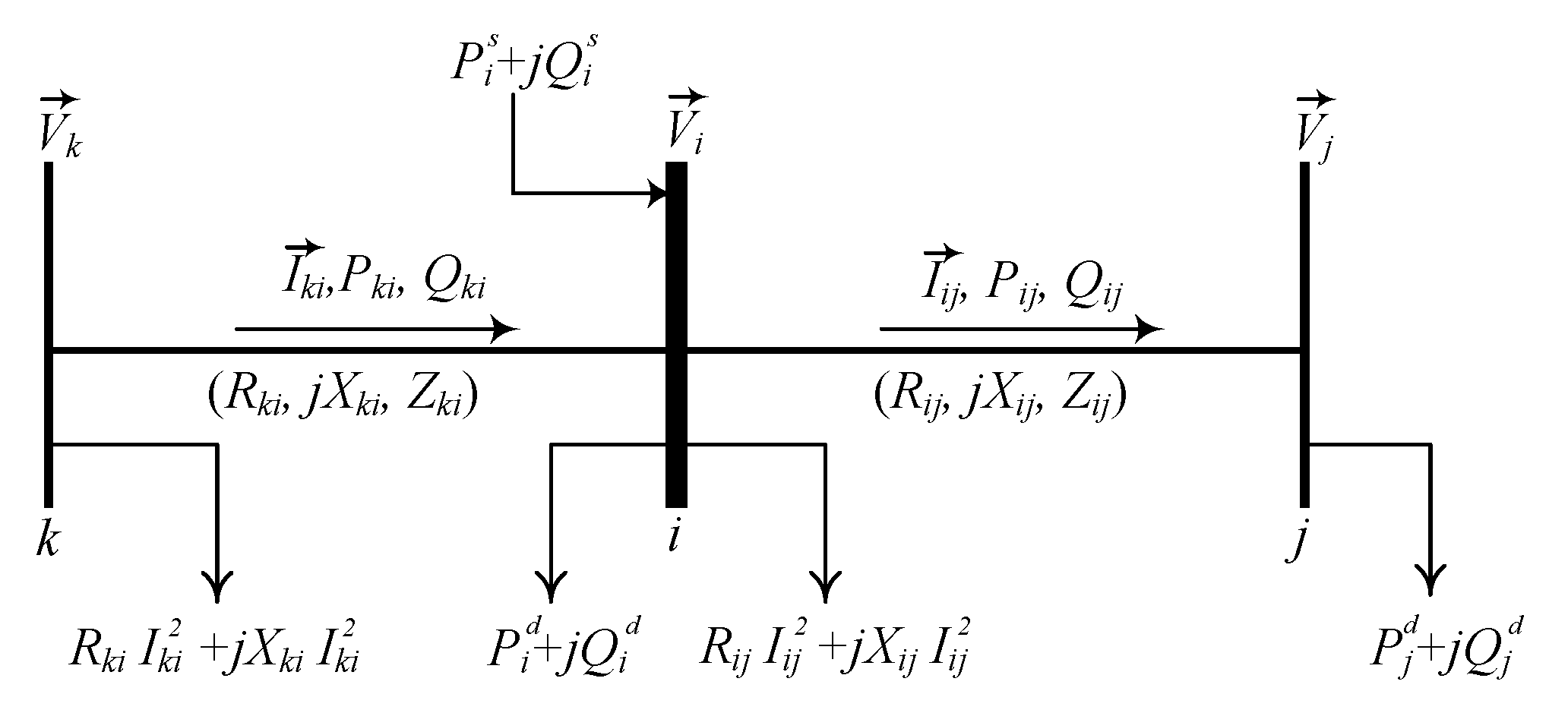
2.1. Mathematical Modeling of the Nonlinear Power Flow

The power flow implemented in this paper is designed for radial EDNs and takes into account the following conditions that represent the steady-state operation of EDNs.

• The topology of the EDN is radial.
• A monophasic equivalent is used to represent the EDN.
• The network demand is modeled as a constant power.
• Only an electric source (substation) is considered.
• The active and reactive power losses of distribution lines are concentrated in their sending bus.
• The capacitive reactance of distribution lines is not taken into account.

The aforementioned conditions are common in most studies regarding the operation and expansion planning of EDNs.

According to Figure 1, the power flow modeling for radial EDNs is given by Equations (1)–(7) [63,64].

$$\hspace{1em}\hspace{1em}\hspace{1em}\begin{array}{c}\mathrm{Minimize}v=k_e{\displaystyle \sum _{\mathsf{\forall }ij\in {\mathsf{\Omega }}_l}}{R}_{ij}{I}_{ij}^2\hfill \\ \mathrm{Subject}\mathrm{to}:\hfill \end{array}$$

(1)

$$\hspace{1em}\hspace{1em}\hspace{1em}\hspace{1em}\hspace{1em}\hspace{1em}\hspace{1em}\hspace{1em}\hspace{1em}\hspace{1em}\hspace{1em}\hspace{1em}\begin{array}{c}\hfill {\displaystyle \sum _{\mathsf{\forall }ki\in {\mathsf{\Omega }}_l}}{P}_{ki}-{\displaystyle \sum _{\mathsf{\forall }ij\in {\mathsf{\Omega }}_l}}\left(P_{ij}+R_{ij}{I}_{ij}^2\right)+P_i^s=P_i^d;\mathsf{\forall }i\in {\mathsf{\Omega }}_b\end{array}$$

(2)

$$\hspace{1em}\hspace{1em}\hspace{1em}\hspace{1em}\hspace{1em}\hspace{1em}\hspace{1em}\hspace{1em}\hspace{1em}\hspace{1em}\hspace{1em}\hspace{1em}\begin{array}{c}{\displaystyle \sum _{\mathsf{\forall }ki\in {\mathsf{\Omega }}_l}}{Q}_{ki}-{\displaystyle \sum _{\mathsf{\forall }ij\in {\mathsf{\Omega }}_l}}\left(Q_{ij}+X_{ij}{I}_{ij}^2\right)+Q_i^s=Q_i^d;\mathsf{\forall }i\in {\mathsf{\Omega }}_b\hfill \end{array}$$

(3)

$$\hspace{1em}\hspace{1em}\hspace{1em}\hspace{1em}\hspace{1em}\hspace{1em}\hspace{1em}\hspace{1em}\hspace{1em}\hspace{1em}\begin{array}{c}{V}_i^2-2\left(R_{ij}{P}_{ij}+X_{ij}{Q}_{ij}\right)-Z_{ij}^2{I}_{ij}^2-V_j^2=0;\mathsf{\forall }ij\in {\mathsf{\Omega }}_l\hfill \end{array}$$

(4)

$$\hspace{1em}\begin{array}{c}{V}_j^2{I}_{ij}^2=P_{ij}^2+Q_{ij}^2;\mathsf{\forall }ij\in {\mathsf{\Omega }}_l\hfill \end{array}$$

(5)

$$\begin{array}{c}0\le I_{ij}\le {\overline{I}}_{ij}\mathsf{\forall }ij\in {\mathsf{\Omega }}_l\hfill \end{array}$$

(6)

$$\begin{array}{c}{{\displaystyle \underline{V}}}_i\le V_i\le {\overline{V}}_i;\mathsf{\forall }i\in {\mathsf{\Omega }}_b\hfill \end{array}$$

(7)

The objective function is given by (1), which consists of minimizing the cost of active power losses, where $k_e$ represents the interest rate of the cost of active power losses, ${\mathsf{\Omega }}_l$ is the set of circuits, while $R_{ij}$ and $I_{ij}$ are the resistance and current of circuit ij, respectively.

Active and reactive power balances at each bus are given by (2) and (3), respectively. $P_{ki}$ and $Q_{ki}$ are the active and reactive power flows in circuit ki, while $P_{ij}$ and $Q_{ij}$ represent active and reactive power flows in circuit ij (kW, kVAr), respectively. $P_i^s$ and $Q_i^s$ represent the active and reactive power supplied by the substation at bus i (kW, kVAr). $P_i^d$ and $Q_i^d$ are the active and reactive power demands at bus i (kW, kVAr). $R_{ij}$ and $X_{ij}$ represent the resistance and reactance of the circuit ij (k$\mathsf{\Omega }$), respectively. Finally, ${\mathsf{\Omega }}_l$ is the set of buses.

Equation (4) takes into account the voltage drop in each circuit ij. Voltage magnitudes are computed using the power flow through the circuit and its electrical parameters. The authors in [65] suggested to eliminate the voltage angle to obtain Equation (4). In this case, $V_i$ represents the voltage magnitude at bus i (kV) and $Z_{ij}$ is the impedance of circuit ij. Equation (5) relates the square of current times the square of voltage, as well as the active and reactive power flows in each circuit ij. Constraints (6) and (7) limit the voltage in buses i and the current through circuits ij, respectively. In this case, ${\overline{V}}_i$ and ${{\displaystyle \underline{V}}}_i$ are the upper and lower voltage limits at bus i (kV), while ${\overline{I}}_{ij}$ and ${{\displaystyle \underline{I}}}_{ij}$ are the the upper and lower current limit of circuit ij (A), respectively.

2.2. Change of Variables

The linearization of (1)–(7) proposed in [63,64] was adapted in this paper. Initially, variables $V_i^2$, $V_j^2$ and $I_{ij}^2$ are replaced by $V_i^{sqr}$, $V_j^{sqr}$, and $I_{ij}^{sqr}$; therefore, the model given by (1) and (7) is modified accordingly.

2.3. Objective Function

The objective function given by Equation (1) is modified according to the change of variable shown in Section 2.2, and includes the minimization of voltage deviation ($\mathsf{\Delta }V$).

$$\begin{array}{c}\hfill Minimize\mathit{v}=k_e{\displaystyle \sum _{\mathsf{\forall }ij\in {\mathsf{\Omega }}_l}}{R}_{ij}{I}_{ij}^{sqr}+{\displaystyle \sum _{i\in {\mathsf{\Omega }}_b}}|V_i-V_i^{nom}|\end{array}$$

(8)

where $V_i$ is the calculated voltage magnitude at bus i and $V_i^{nom}$ is the nominal voltage in p.u. In this case, the voltage profile improves as ($\mathsf{\Delta }V$) is lower.

2.4. Active Power Balance Constraints

The active power balance constraint given by Equation (2) is modified as follows to include $P_{ic,g}^{dg}$, which represents the active power injected by the DG unit at candidate bus ic:

$$\begin{array}{cc}\hfill & {\displaystyle \sum _{\mathsf{\forall }ki\in {\mathsf{\Omega }}_l}}{P}_{ki}-{\displaystyle \sum _{\mathsf{\forall }ij\in {\mathsf{\Omega }}_l}}(P_{ij}+R_{ij}{I}_{ij}^{sqr})+P_i^s+{\displaystyle \sum _{g\in {\mathsf{\Omega }}_g}}{P}_{ic,g}^{dg}=P_i^d;\mathsf{\forall }i\in {\mathsf{\Omega }}_b,\mathsf{\forall }ic\in {\mathsf{\Omega }}_{bc}\hfill \end{array}$$

(9)

2.5. Reactive Power Balance Constraints

The reactive power balance constraint given by Equation (3) is modified as follows to include $Q_{ic,g}^{dg}$, which represents the reactive power injected by the DG unit at candidate bus ic:

$$\begin{array}{cc}\hfill & {\displaystyle \sum _{\mathsf{\forall }ki\in {\mathsf{\Omega }}_l}}{Q}_{ki}-{\displaystyle \sum _{\mathsf{\forall }ij\in {\mathsf{\Omega }}_l}}(Q_{ij}+X_{ij}{I}_{ij}^{sqr})+Q_i^s+{\displaystyle \sum _{g\in {\mathsf{\Omega }}_g}}{Q}_{ic,g}^{dg}=Q_i^d;\mathsf{\forall }i\in {\mathsf{\Omega }}_b,\mathsf{\forall }ic\in {\mathsf{\Omega }}_{bc}\hfill \end{array}$$

(10)

2.6. Voltage Drop in Circuits

The voltage drop in circuits given by Equation (4) is modified as follows to consider the optimal reconfiguration:

$$\begin{array}{cc}\hfill & V_i^{sqr}-2(R_{ij}{P}_{ij}+X_{ij}{Q}_{ij})-Z_{ij}^2{I}_{ij}^{sqr}-V_j^{sqr}-b_{ij}=0;\mathsf{\forall }ij\in {\mathsf{\Omega }}_l\hfill \end{array}$$

(11)

where $b_{ij}$ is an auxiliary variable that takes different values when the circuit ij is open or closed.

2.7. Linearization

Applying the change of variable proposed in Section 2.2, the left-hand side of Equation (5) can be rewritten and linearized as follows [63]:

$$\begin{array}{cc}\hfill & V_j^{sqr}{I}_{ij}^{sqr}=\left({{\displaystyle \underline{V}}}^2+\frac{1}{2}{\overline{\mathsf{\Delta }}}^V\right)I_{ij}^{sqr}+\sum _{s=1}^S{P}_{j,s}^c;\mathsf{\forall }ij\in {\mathsf{\Omega }}_l\hfill \end{array}$$

(12)

$$\begin{array}{cc}\hfill & {{\displaystyle \underline{V}}}^2+\sum _{s=1}^S\left(x_{j,s}{\overline{\mathsf{\Delta }}}^V\right)\le V_j^{sqr}\le {{\displaystyle \underline{V}}}^2+\sum _{s=1}^S\left(x_{j,s}{\overline{\mathsf{\Delta }}}^V\right)+{\overline{\mathsf{\Delta }}}^V;\mathsf{\forall }j\in {\mathsf{\Omega }}_b\hfill \end{array}$$

(13)

$$\begin{array}{cc}\hfill & x_{j,s}\le x_{j,s-1};\mathsf{\forall }j\in {\mathsf{\Omega }}_b;s=2...S\hfill \end{array}$$

(14)

$$\begin{array}{cc}\hfill & x_{j,s}\in \left\{0,1\right\};\mathsf{\forall }j\in {\mathsf{\Omega }}_b;s=1...S\hfill \end{array}$$

(15)

$$\begin{array}{cc}\hfill & 0\le {\overline{\mathsf{\Delta }}}^V{I}_{ij}^{sqr}-P_{j,s}^c\le {\overline{\mathsf{\Delta }}}^V{\overline{I}}_{ij}^{sqr}\left(1-x_{j,s}\right);\mathsf{\forall }ij\in {\mathsf{\Omega }}_l,s=1...S\hfill \end{array}$$

(16)

$$\begin{array}{cc}\hfill & 0\le P_{j,s}^c\le {\overline{\mathsf{\Delta }}}^V{\overline{I}}_{ij}^{sqr}{x}_{j,s};\mathsf{\forall }ij\in {\mathsf{\Omega }}_l\hfill \end{array}$$

(17)

In this case, S represents the number of discretizations; ${\overline{\mathsf{\Delta }}}^V$ is the discretization step, and $x_{j,s}$ is the binary variable used in the discretization of $V_j^{sqr}$. The variable $P_{j,s}^c$ is the power correction factor.

The right-hand side of (5) can be linearized as follows [63]:

$$\begin{array}{cc}\hfill & P_{ij}^2+Q_{ij}^2=\sum _{y=1}^Y{m}_{ij,y}^s·\mathsf{\Delta }{P}_{ij,y}+\sum _{y=1}^Y{m}_{ij,y}^s·\mathsf{\Delta }{Q}_{ij,y};\mathsf{\forall }ij\in {\mathsf{\Omega }}_l\hfill \end{array}$$

(18)

$$\begin{array}{cc}\hfill & P_{ij}^{+}-P_{ij}^{-}=P_{ij};\mathsf{\forall }ij\in {\mathsf{\Omega }}_l\hfill \end{array}$$

(19)

$$\begin{array}{cc}\hfill & P_{ij}^{+}+P_{ij}^{-}=\sum _{y=1}^Y\mathsf{\Delta }{P}_{ij,y};\mathsf{\forall }ij\in {\mathsf{\Omega }}_l\hfill \end{array}$$

(20)

$$\begin{array}{cc}\hfill & 0\le \mathsf{\Delta }{P}_{ij,y}\le {\overline{△S}}_{ij};\mathsf{\forall }ij\in {\mathsf{\Omega }}_l,\mathsf{\forall }y\in 1...Y\hfill \end{array}$$

(21)

$$\begin{array}{cc}\hfill & 0\le P_{ij}^{+};\mathsf{\forall }ij\in {\mathsf{\Omega }}_l\hfill \end{array}$$

(22)

$$\begin{array}{cc}\hfill & 0\le P_{ij}^{-};\mathsf{\forall }ij\in {\mathsf{\Omega }}_l\hfill \end{array}$$

(23)

$$\begin{array}{cc}\hfill & Q_{ij}^{+}-Q_{ij}^{-}=Q_{ij};\mathsf{\forall }ij\in {\mathsf{\Omega }}_l\hfill \end{array}$$

(24)

$$\begin{array}{cc}\hfill & Q_{ij}^{+}+Q_{ij}^{-}=\sum _{y=1}^Y\mathsf{\Delta }{Q}_{ij,y};\mathsf{\forall }ij\in {\mathsf{\Omega }}_l\hfill \end{array}$$

(25)

$$\begin{array}{cc}\hfill & 0\le \mathsf{\Delta }{Q}_{ij,y}\le {\overline{△S}}_{ij};\mathsf{\forall }ij\in {\mathsf{\Omega }}_l,\mathsf{\forall }y\in 1...Y\hfill \end{array}$$

(26)

$$\begin{array}{cc}\hfill & 0\le Q_{ij}^{+};\mathsf{\forall }ij\in {\mathsf{\Omega }}_l\hfill \end{array}$$

(27)

$$\begin{array}{cc}\hfill & 0\le Q_{ij}^{-};\mathsf{\forall }ij\in {\mathsf{\Omega }}_l\hfill \end{array}$$

(28)

As regards the linearization of $P_{ij}^2$ and $Q_{ij}^2$, the following variables are considered: Y represents the number of blocks of the piece-wise linearization; $m_{ij,y}^s$ is the slope of the $y_{th}$ block of the power flow at circuit ij; $\mathsf{\Delta }{P}_{ij,y}$ and $\mathsf{\Delta }{Q}_{ij,y}$ represent the values of the $y_{th}$ block of $\left|P_{ij}\right|$ and $\left|Q_{ij}\right|$, respectively; $\overline{\mathsf{\Delta }}{S}_{ij}$ is the upper limit of each block of the power flow at circuit ij; $P_{ij}^{+}$ and $P_{ij}^{-}$ represent positive auxiliary variables used to compute $\left|P_{ij}\right|$; and $Q_{ij}^{+}$ and $Q_{ij}^{-}$ represent positive auxiliary variables used to compute $\left|Q_{ij}\right|$. The values of $m_{ij,y}^s$ and $\overline{\mathsf{\Delta }}{S}_{ij}$ are calculated as indicated in Equations (28) and (29).

$$\begin{array}{cc}\hfill & m_{ij,y}^s=\left(2y-1\right)\overline{\mathsf{\Delta }}{S}_{ij}\hfill \end{array}$$

(29)

$$\begin{array}{cc}\hfill & \overline{\mathsf{\Delta }}{S}_{ij}=\overline{V}·{\overline{I}}_{ij}/Y\hfill \end{array}$$

(30)

Following the linearization presented above, Equation (5) assumes the following form:

$$\begin{array}{cc}\hfill & \left({{\displaystyle \underline{V}}}^2+\frac{1}{2}{\overline{\mathsf{\Delta }}}^V\right)I_{ij}^{sqr}+\sum _{s=1}^S{P}_{j,s}^c=\sum _{y=1}^Y{m}_{ij,y}^s·\mathsf{\Delta }{P}_{ij,y}+\sum _{y=1}^Y{m}_{ij,y}^s·\mathsf{\Delta }{Q}_{ij,y};\mathsf{\forall }ij\in {\mathsf{\Omega }}_l\hfill \end{array}$$

(31)

2.8. Voltage and Current Limits

Equations (6) and (7) are modified as indicated in (31) and (32) taking into account the change of variable described in Section 2.2.

$$\begin{array}{cc}\hfill & 0\le I_{ij}^{sqr}\le {\overline{I}}_{ij}^2\mathsf{\forall }ij\in {\mathsf{\Omega }}_l\hfill \end{array}$$

(32)

$$\begin{array}{cc}\hfill & {{\displaystyle \underline{V}}}_i^2\le V_i^{sqr}\le {\overline{V}}_i^2;\mathsf{\forall }i\in {\mathsf{\Omega }}_b\hfill \end{array}$$

(33)

2.9. Constraints Related to the DNR Problem

The current limit in circuits represented by the constraint (32) is modified according to (33). Moreover, constraints (35) to (41) are added to the model for considering the optimal DNR.

$$\begin{array}{cc}\hfill & 0\le I_{ij}^{sqr}\le {\overline{I}}_{ij}^2\left(y_{ij}^{+}+y_{ij}^{-}\right);\mathsf{\forall }ij\in {\mathsf{\Omega }}_l\hfill \end{array}$$

(34)

$$\begin{array}{cc}\hfill & 0\le P_{ij}^{+}\le \overline{V}\overline{I}{y}_{ij}^{+};\mathsf{\forall }ij\in {\mathsf{\Omega }}_l;\mathsf{\forall }ij\in {\mathsf{\Omega }}_l\hfill \end{array}$$

(35)

$$\begin{array}{cc}\hfill & 0\le P_{ij}^{-}\le \overline{V}\overline{I}{y}_{ij}^{-};\mathsf{\forall }ij\in {\mathsf{\Omega }}_l;\mathsf{\forall }ij\in {\mathsf{\Omega }}_l\hfill \end{array}$$

(36)

$$\begin{array}{cc}\hfill & |Q_{ij}|\le \overline{V}\overline{I}\left(y_{ij}^{+}+y_{ij}^{-}\right);\mathsf{\forall }ij\in {\mathsf{\Omega }}_l\hfill \end{array}$$

(37)

$$\begin{array}{cc}\hfill & |b_{ij}|\le \left({\overline{V}}^2-{{\displaystyle \underline{V}}}^2\right)\left(1-\left(y_{ij}^{+}+y_{ij}^{-}\right)\right);\mathsf{\forall }ij\in {\mathsf{\Omega }}_l\hfill \end{array}$$

(38)

$$\begin{array}{cc}\hfill & {\displaystyle \sum _{ij\in {\mathsf{\Omega }}_l}}\left(y_{ij}^{+}+y_{ij}^{-}\right)=N-1;\mathsf{\forall }ij\in {\mathsf{\Omega }}_l\hfill \end{array}$$

(39)

$$\begin{array}{cc}\hfill & \left(y_{ij}^{+}+y_{ij}^{-}\right)\le 1;\mathsf{\forall }ij\in {\mathsf{\Omega }}_l\hfill \end{array}$$

(40)

$$\begin{array}{cc}\hfill & y_{ij}^{+};y_{ij}^{-};binary;\mathsf{\forall }ij\in {\mathsf{\Omega }}_l\hfill \end{array}$$

(41)

In this case, $b_{ij}$ is an auxiliary variable, which is zero if circuit ij is closed according to Equation (38); otherwise, this variable is free to take values within the constraint given by Equation (39) to comply with Equation (40); $y_{ij}^{+}$ and $y_{ij}^{-}$ represent binary variables related to the power flow direction of circuit ij. If both variables are equal to zero, the circuit is open; if any variable is equal to one, it means the switch in this circuit is closed. Equation (39) guarantees that the EDN is radial. Equation (40) allows one of the binary variables related to the load flow direction at circuit ij to be equal to one. Finally, N indicates the number of buses of the EDN.

2.10. Constraints Related to the OPDG

The following linear constraints are added to the model to consider the OPDG:

$$\begin{array}{cc}\hfill & {{\displaystyle \underline{P}}}_g^{gd}·W_{ic,g}^{gd}\le P_{ic,g}^{gd}\le {\overline{P}}_g^{gd}·W_{ic,g}^{gd};{\mathsf{\forall }}_{ic}\in {\mathsf{\Omega }}_{bc},{\mathsf{\forall }}_g\in {\mathsf{\Omega }}_g\hfill \end{array}$$

(42)

$$\begin{array}{cc}\hfill & |Q_{ic,g}^{dg}|\le P_{ic,g}^{dg}·tan(arccos\left({\varphi }_g\right));{\mathsf{\forall }}_{ic}\in {\mathsf{\Omega }}_{bc},{\mathsf{\forall }}_g\in {\mathsf{\Omega }}_g\hfill \end{array}$$

(43)

$$\begin{array}{cc}\hfill & {{\displaystyle \underline{Q}}}_{ic,g}^{dg}\le Q_{ic,g}^{dg}\le {\overline{Q}}_{ic,g}^{dg};{\mathsf{\forall }}_{ic}\in {\mathsf{\Omega }}_{bc},{\mathsf{\forall }}_g\in {\mathsf{\Omega }}_g\hfill \end{array}$$

(44)

$$\begin{array}{cc}\hfill & {\left(P_{ic,g}^{dg}\right)}^2+{\left(Q_{ic,g}^{dg}\right)}^2\le {\left(S_{ic,g}^{dg}\right)}^2;{\mathsf{\forall }}_{ic}\in {\mathsf{\Omega }}_{bc},{\mathsf{\forall }}_g\in {\mathsf{\Omega }}_g\hfill \end{array}$$

(45)

$$\begin{array}{cc}\hfill & {\displaystyle \sum _{g\in {\mathsf{\Omega }}_g}}{W}_{ic,g}^{gd}\le 1;{\mathsf{\forall }}_{ic}\in {\mathsf{\Omega }}_{bc}\hfill \end{array}$$

(46)

$$\begin{array}{cc}\hfill & {\displaystyle \sum _{ic\in {\mathsf{\Omega }}_{bc}}}{\displaystyle \sum _{g\in {\mathsf{\Omega }}_g}}{W}_{ic,g}^{gd}\le {\overline{N}}_{syst}^{dg}\hfill \end{array}$$

(47)

$$\begin{array}{cc}\hfill & W_{ic,g}^{dg}\in \{0,1\};{\mathsf{\forall }}_{ic}\in {\mathsf{\Omega }}_{bc},{\mathsf{\forall }}_g\in {\mathsf{\Omega }}_g\hfill \end{array}$$

(48)

where $W_{ic,g}^{dg}$ (binary variable) indicates if a DG unit of type g is placed at candidate bus ic. $P_{ic,g}^{gd}$ and $Q_{ic,g}^{gd}$ (indicate) the active and reactive power injected by DG unit of type g (kW, kVAr). ${{\displaystyle \underline{P}}}_{ic,g}^{dg}$ and ${\overline{P}}_{ic,g}^{dg}$ represent the minimum and maximum limits of the active power injected by a DG unit (kW) of type g at candidate bus ic, ${{\displaystyle \underline{Q}}}_{ic,g}^{dg}$ and ${\overline{Q}}_{ic,g}^{dg}$ represent the minimum and maximum limits of reactive power supplied by the DG unit (kVar) of type g at candidate bus ic, and $S_{ic,g}^{dg}$ is the apparent power injected by DG of type g at candidate bus ic (kVA). ${\varphi }_g$ is the power factor of DG type g.

2.11. MILP Model for Optimal DNR and OPDG

The proposed MILP model for DNR and OPDG consists on minimizing active power losses given by Equation (8), subject to: active and reactive power balance constratins given by Equations (9) and (10); voltage drop constraint given by Equation (11); linealization of Equation (5) which relates the square of current times the square of voltage through Equations (13)–(17) that linealize the left-hand side, Equations (19)–(28) that linealize the right-hand side, and Equation (31) that relates both sides of Equation (5); voltage and current limit constraints given by Equations (32) and (33); DNR problem constraints given by Equations (34)–(41); and finally, OPGD constraints given by Equations (42)–(48).

It is worth mentioning that in some market models, the decision regarding the location of DG in EDNs does not depend on the distribution system operator (DSO); therefore, the location of DG units is an input to the DNR problem. In this case, the DSO may find an optimal reconfiguration that would maximize the benefits of the DG located within its network. Furthermore, the location of DG units might be limited to a subset of nodes due to the availability of resources. In this case, the model can be adapted to find the optimal location of DG units within this new subset and obtain the optimal DNR that minimizes total power losses and voltage deviation.

3. Tests and Results

The presented mathematical model was written in the AMPL programming language and solved using CPLEX. Distribution test systems of 16, 33, 69, 83, 136, and 202 buses were used to prove the applicability of the proposed model. The electrical data of the tested systems are available in [66]. On a computer with an Intel i7-8850H processor, all simulations were run.

All simulations take into account the following hypotheses:

1.

The interest rate of the cost of active power losses ($k_e$) is equal to 168 US$/kW-year [67].

2.

The power injected by the GD units will be 20% of the total power demand of the electrical system tested.

3.

For each test system, a subset of buses is defined as candidates for DG allocation. This is done to present the availability of primary energy resources within a given area.

4.

The size of the DG units is determined by the primary energy resources available; therefore, it must be considered as input data. This must be done based on studies carried out by each distribution system operator or GD owner.

5.

There is a group of generation technologies that can be applied in DG applications. For illustrative purposes, two types of DG units are considered: Type 1 operates at a 0.95 lagging power factor, and Type 2 operates at a unity power factor. Nonetheless, any other type of DG may be also considered in the formulation.

3.1. Comparative Analysis between Linear and Nonlinear Power Flow

The proposed model for the simultaneous optimal DNR and OPDG (Section 2.11) includes the linearization of the power flow. To assess the effectiveness of this linear power flow, a comparison was carried out with its conventional nonlinear counterpart described in Section 2.1. The computational codes of both models were implemented in the AMPL programming language. The nonlinear power flow was solved using KNITRO software, while the linear power flow was solved using CPLEX. This latter software is proven to be more effective when solving the proposed model, especially for real-size EDNs.

Table 1. Nonlinear vs. linear power flow model.

Test System	Parameter	Power Flow Model		Relative Error (%)
		Nonlinear	Linear
14-bus	Y	–	50	–
	S	–	3	–
	Power losses (kW)	511.43	511.23	0.0391
	Vmin (p.u.)	0.9692	0.9692	0.0000
	Time (s)	0.0004	0.0002	–
33-bus	Y	–	50	–
	S	–	4	–
	Power losses (kW)	202.56	202.67	0.0543
	Vmin (p.u.)	0.9130	0.9130	0.0000
	Time (s)	0.0024	0.0009	–
69-bus	Y	–	70	–
	S	–	6	–
	Power losses (kW)	224.57	224.99	0.1870
	Vmin (p.u.)	0.9091	0.9092	0.0110
	Time (s)	0.0015	0.0003	–
83-bus	Y	–	50	–
	S	–	3	–
	Power losses (kW)	532.08	531.99	0.0169
	Vmin (p.u.)	0.9285	0.9285	0.0000
	Time (s)	0.0031	0.0004	–
119-bus	Y	–	100	–
	S	–	5	–
	Power losses (kW)	1296.28	1296.57	0.0224
	Vmin (p.u.)	0.8688	0.8687	0.0115
	Time (s)	0.0154	0.0006	–
136-bus	Y	–	50	–
	S	–	3	–
	Power losses (kW)	320.90	320.36	0.1683
	Vmin (p.u.)	0.9306	0.9306	0.0000
	Time (s)	0.0047	0.0005	–
202-bus	Y	–	80	–
	S	–	5	–
	Power losses (kW)	548.26	548.89	0.1149
	Vmin (p.u.)	0.9571	0.9574	0.0313
	Time (s)	0.00128	0.0007	–

presents a comparison of results between the linear and nonlinear power flow models. The number of piece-wise linearizations (Y) and discretizations (S) used in the linear power flow model was determined by running several simulations with different values of these parameters for each test system. For all EDNs, the linear model obtains similar solutions (power losses and minimum voltage) to the exact model; nonetheless, it has lower computational time.

It is worth mentioning that the selection of Y and S is a key factor in the performance of the model. On one hand, low values of these parameters result in a lack of accuracy with respect to the nonlinear original model; on the other hand, high values of these parameters may lead to convergence problems due to an increased number of constraints (especially for large EDNs). This was not our case, since a proper selection of these parameters was carried out for each test system (see Table 1).

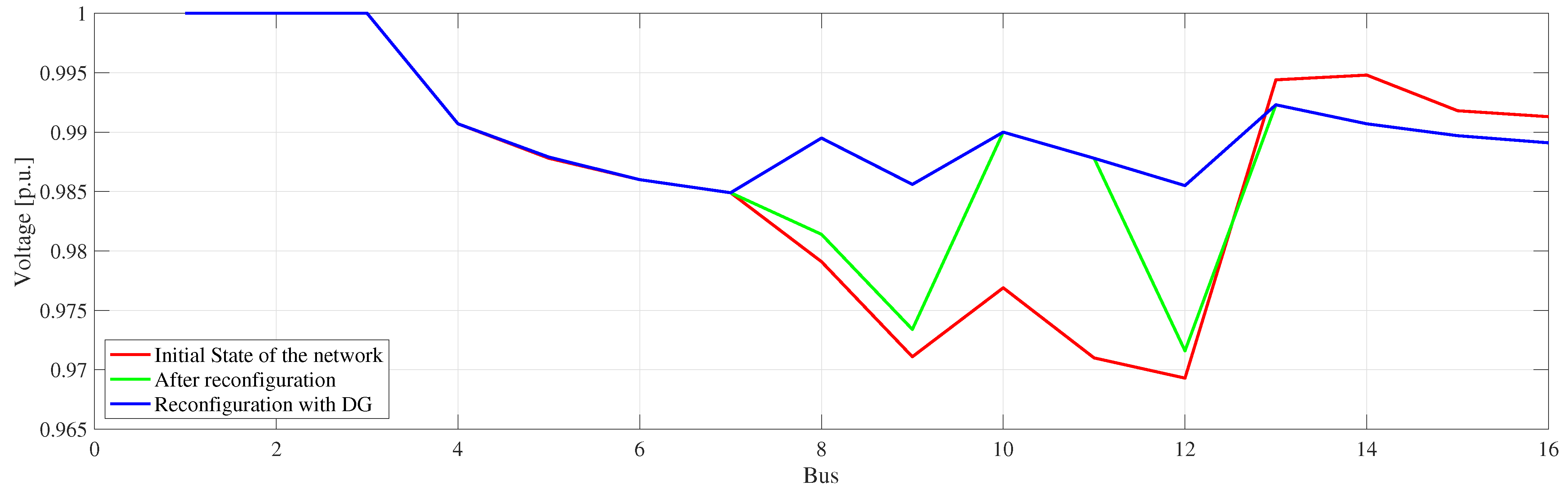
3.2. Case Study I: 16-Bus Test System

This distribution system features 16 circuits with 13 tie switches and 3 normally open interconnection switches. The data of this system can be consulted in [66]. In its initial topology, switches 15, 21, and 23 are open. The nominal voltage of this system is 23 kV, and it must supply a load of (28,700 + j17,300) kVA. The initial value of active power losses (without reconfiguration) is 511.4321 kW.

Table 2. Results for the 16-bus test system.

Case	Open Switches	DG Data				Power Losses	Reduction (%)	Vmin (p.u.)	$\mathbf{\Delta }\mathit{V}$	Time (s)
		Type	P (kW)	Q (kVAr)	Bus
I	15, 21, 23	–	–	–	–	511.43	–	0.9692	0.2109	–
II	17, 19, 26	–	–	–	–	466.12	8.85	0.9715	0.1845	0.09
III	17, 19, 26	1	1740	571.91	8	252.95	50.64	0.9849	0.1503	0.1042
		1	2000	657.36	9
		2	2000	–	12

presents the open switches for the initial topology and the optimal solution found by the proposed mathematical model. Note that power losses present a reduction of 8.85%. In this case, the CPU time is 0.09 s. The solution found for the proposed model to the optimal reconfiguration problem is the same as reported in [33,68]. On the other hand, the optimal reconfiguration considering DG units proposes to install two units of Type 1 at buses 8 and 9 with a power of $(1740+j571.91)$ kVA and $(2000+j657.36)$ kVA, and one Type 2 unit at bus 12 with an active power of 2000 kW. When DG units are included, active power losses present a reduction of 50.64%, and the CPU time is 0.1042 s. Note that in both cases, with and without DG, the system topology remains the same; nonetheless, the power loss reduction is higher when DG is considered. As regards voltage deviation, it improves from 0.2109 in case 1 to 0.1503 in case 3.

Figure 2 depicts the voltage profile of the initial state (base case) of the EDN, and the voltage profile after reconfiguration with and without DG. It can be noted that the voltage profiles have been enhanced as a result of the optimal reconfiguration and with the reconfiguration considering DG.

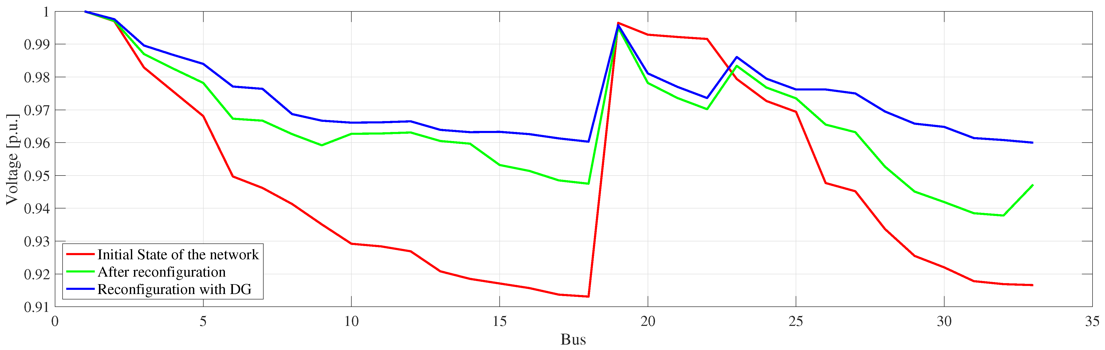
3.3. Case Study II: 33-Bus Test System

This distribution system features 37 circuits with 32 tie switches and 5 normally open interconnection switches. The data of this system can be consulted in [66]. In its initial topology, switches 33, 34, 35, 36, and 37 are open. The nominal voltage is 12.66 kV and the system must supply a load of (3715 + j2300) kVA. The initial value of active power losses (without reconfiguration) is 202.6771 kW.

Table 3. Results for the 33-bus test system.

Case	Open Switches	DG Data				Power Losses	Reduction (%)	Vmin (p.u.)	$\mathbf{\Delta }\mathit{V}$	Time (s)
		Type	P (kW)	Q (kVAr)	Bus
I	33, 34, 35, 36, 37	–	–	–	–	202.67	–	0.9131	1.7007	–
II	7, 9, 14, 32, 37	–	–	–	–	139.54	31.15	0.9378	1.1473	0.46
III	7, 9, 14, 32, 37	1	544.41	178.94	30	83.67	58.71	0.9600	0.8770	6.95
		2	178.58	–	17

indicates the open switches, active power losses, percentage of active power losses reduced, minimum voltage, voltage deviation, and CPU time of the initial topology, and the optimal solutions found by the proposed mathematical model with and without DG units. In the case of optimal reconfiguration, the active power losses present a reduction of 31.15%, the minimum voltage rises from 0.9131 to 0.9378 p.u., and the CPU time is 0.46 s. On the other hand, the optimal reconfiguration considering DG proposes to install one Type 1 unit at bus 30 with a power of $(544.41+j178.94)$ kVA, and one Type 2 unit at bus 17 with an active power of $198.58$ kW. In this case, the active power losses present a reduction of 58.71%, the minimum voltage is 0.96 p.u., and the CPU time is 6.95 s. Note that in this case, the voltage deviation is only 0.8770 compared to 1.7007 (base case).

Figure 3 presents the voltage profile of the initial state (base case) of the EDN, and the voltage profile after reconfiguration with and without DG. It can be noted that voltage profiles are improved with optimal reconfiguration and with the reconfiguration considering DG.

3.4. Case Study III: 69-Bus Test System

This distribution system features 73 circuits with 68 tie switches and 5 normally open interconnection switches. The data of this system can be consulted in [66]. In its initial topology, switches 69, 70, 71, 72, and 73 are open. The nominal voltage of this 69-bus test system is 12.66 kV, and it must supply a load of (3802.19 + j2694.6) kVA. The initial value of active power losses (without reconfiguration) is 224.99 kW.

Table 4. Results for the 69-bus test system.

Case	Open Switches	DG Data				Power Losses	Reduction (%)	Vmin (p.u.)	$\mathbf{\Delta }\mathit{V}$	Time (s)
		Type	P (kW)	Q (kVAr)	Bus
I	69, 70, 71, 72, 73	–	–	–	–	224.99	–	0.9092	1.8371	–
II	14, 55, 61, 69, 70	–	–	–	–	99.62	55.72	0.9427	1.0234	2.42
III	14, 58, 62, 69, 70	1	260.43	85.61	61	50.64	77.49	0.9649	0.7990	3.09
		1	500.00	164.34	64

shows the open switches for the initial topology, and the optimal solution found by the proposed mathematical model. Note that power losses present a reduction of 55.72% and the minimum voltage of the network goes from 0.9092 to 0.9427 p.u. In this case, the CPU time is 2.42 s. The optimal reconfiguration considering DG proposes to install two Type 1 units at buses 61 and 64 with a power of $(260.43+j85.61)$ kVA, and $(500+164.34)$ kVA, respectively. Nonetheless, Type 2 units are not installed. When DG is included in the reconfiguration process, the active power losses present a reduction of 77.49%, the voltage deviation is 0.7990, compared to 1.8371 (base case), and the CPU time is 3.09 s. As regards network topology, only the status of switch 56 is different with and without DG.

Figure 4 shows three voltage profiles indicating the initial state (base case) of the network, the system with reconfiguration, and the system with reconfiguration and DG. Note that an important improvement is achieved after reconfiguration, especially in the last buses of the network. In this case, the impact of DG in the voltage profile is only noted in buses 51 to 64.

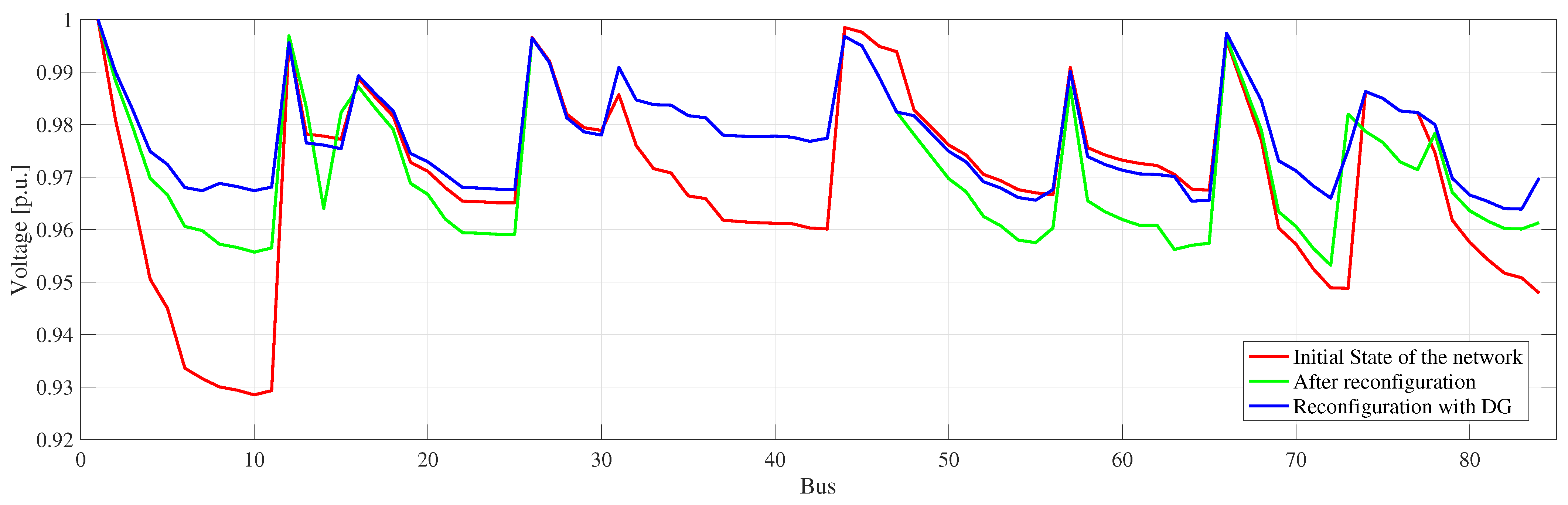
3.5. Case Study IV: 83-Bus Test System

This distribution system features 96 circuits with 83 tie switches and 13 normally open interconnection switches. The data of this system can be consulted in [66]. In its initial topology, switches 84, 85, 86, 87, 88, 89, 90, 91, 92, 93, 94, 95, and 96 are open. The nominal voltage is 11.4 kV, and the system must supply a load of $(28,350.9+20,700)$ kVA. The initial value of active power losses (without reconfiguration) is 531.99 kW.

Table 5. Results for the 83-bus test system.

Case	Open Switches	DG Data				Power Losses	Reduction (%)	Vmin (p.u.)	$\mathbf{\Delta }\mathit{V}$	Time (s)
		Type	P (kW)	Q (kVAr)	Bus
I	84, 85, 86, 87, 88, 89, 90, 91, 92, 93, 94, 95, 96	–	–	–	–	531.99	–	0.9285	2.5589	–
II	7, 13, 34, 39, 42, 55, 61, 72, 82, 86, 89, 90, 92	–	–	–	–	469.87	11.67	0.9532	2.3119	2.58
III	7, 34, 39, 42, 55, 63, 72, 83, 86, 88,	1	1000.00	328.68	7	313.40	41.08	0.9638	1.9265	25.76
	89, 90, 92	1	1000.00	328.68	20
		1	1000.00	328.68	71
		2	908.20	–	6
		2	1000.00	–	53
		2	761.97	–	70

shows the open switches, active power losses, percentage of active power losses reduced, minimum voltage, voltage deviation, and CPU time of the initial topology, and the optimal solutions found by the proposed mathematical model with and without DG units. In the case of optimal reconfiguration, the active power losses present a reduction of 11.67%, the minimum voltage improves from 0.9285 to 0.9532 p.u., and the CPU time is 2.58 s. On the other hand, the model for optimal reconfiguration considering DG proposes to install three Type 1 units at buses 7, 20, and 71 with a power of $(1000+j328.68)$ kVA, and three Type 2 units at buses 6, 53, and 70 with an active power of $908.20$ kW, 1000 kW, and $761.97$ kW, respectively. In this case, the active power losses have a reduction of 41.08%, the minimum voltage is 0.9638 p.u., the voltage deviation improves from 2.5589 (base case) to 1.9265, and the CPU time is 25.76 s. Note that the topology of the reconfiguration considering DG differs only in one switch with respect to the case where DG is not considered.

Figure 5 shows the voltage profile of the initial state (base case) of the EDN, and the voltage profile after reconfiguration with and without DG. It can be noted that the voltage profiles have been enhanced as a result of the reconfiguration process and even further improved when DG is considered.

3.6. Case Study V: 119-Bus Test System

This distribution system features 133 circuits with 118 tie switches and 15 normally open interconnection switches. The data of this system can be consulted in [66]. In its initial topology, switches 119, 120, 121, 122, 123, 124, 125, 126, 127, 128, 129, 130, 131, 132, and 133 are open. The nominal voltage is 11 kV, and the system must supply a load of $(22,709.72+j17,041.067)$ kVA. The initial value of active power losses (without reconfiguration) is 1296.57 kW.

Table 6. Results for the 119-bus test system.

Case	Open Switches	DG Data				Power Losses	Reduction (%)	Vmin (p.u.)	$\mathbf{\Delta }\mathit{V}$	Time (s)
		Type	P (kW)	Q (kVAr)	Bus
I	119, 120, 121, 122, 123, 124, 125, 126, 127, 128, 129, 130, 131, 132, 133	–	–	–	–	1296.57	–	0.8687	5.2403	–
II	24, 27, 35, 40, 43, 52, 59, 72, 75, 96, 98, 110, 123, 130, 131	–	–	–	–	869.71	32.92	0.9321	3.7736	3.82
III	23, 26, 35, 40, 43, 52, 61, 72, 77,	1	1000	328.58	52	529.94	59.12	0.9556	2.9972	1709.95
	83, 110, 122, 126, 127, 131	1	1000	328.67	77
		1	918.03	301.74	116
		2	1000	–	83
		2	1000	–	101

shows the open switches, active power losses, percentage of active power losses reduced, minimum voltage, and CPU time of the initial topology, and the optimal solutions found by the proposed mathematical model with and without DG units. In the case of optimal reconfiguration, the active power losses present a reduction of 32.92%, the minimum voltage of the network improves from 0.8687 to 0.9321 p.u., and the CPU time is 3.82 s. On the other hand, the optimal reconfiguration considering DG units proposes to install two Type 1 units at buses 52 and 77 with a power of $(1000+j328.58)$ kVA and one at bus 116 with a power of $(918.03+j301.74)$ kVA. Moreover, there are two Type 2 units at buses 83 and 101 with an active power of $785.09$ kW and $838.82$ kW, respectively. In this case, active power losses present a reduction of 59.12%, the voltage deviation improves from 5.2403 (base case) to 2.9972, and the CPU time is 1709.95 s. Note that the topology is different for the reconfiguration with and without DG.

Figure 6 shows the voltage profile of the initial state (base case) of the EDN, and the voltage profile after reconfiguration with and without DG. It can be seen that the voltage profiles have been enhanced as a result of the optimal reconfiguration, and with the reconfiguration considering DG.

3.7. Case Study V: 136-Bus test System

This distribution system features 156 circuits with 135 tie switches and 21 normally open interconnection switches. The data of this system can be consulted in [66]. In its initial topology, switches 136, 137, 138, 139, 140, 141, 142, 143, 144, 145, 146, 147, 148, 149, 150, 151, 152, 153, 154, 155, and 156 are open. The nominal voltage is 13.8 kV, and the system must supply a load of ($\mathrm{18,313.8}+j7932.5$) kVA. The initial value of active power losses (without reconfiguration) is 320.36 kW.

Table 7. Results for the 136-bus test system.

Case	Open Switches	DG Data				Power Losses	Reduction (%)	Vmin (p.u.)	$\mathbf{\Delta }\mathit{V}$	Time (s)
		Type	P (kW)	Q (kVAr)	Bus
I	135, 136, 137, 138, 139, 140, 141, 142, 143, 144, 145, 146, 147, 148, 149, 150, 151, 152, 153, 154, 155, 156	–	–	–	–	320.36	–	0.9306	3.4073	–
II	7, 35, 51, 90, 96, 106, 118, 126, 135, 137, 138, 141, 142, 144, 145, 146, 147, 148, 150, 151, 155	–	–	–	–	280.19	12.55	0.9581	3.0802	7.07
III	51, 54, 83, 84, 90, 96, 106, 120, 126,	1	982.33	322.87	35	169.74	47.01	0.9719	2.5107	113.85
	128, 135, 136, 137, 139, 141, 144,	1	1000	328.68	155
	145, 147, 148, 150, 151	2	924.82	–	17
		2	755.60	–	157

shows the open switches, active power losses, percentage of active power losses reduced, minimum voltage, voltage deviation, and CPU time of the initial topology, and the optimal solutions found by the proposed mathematical model with and without DG units. In the case of optimal reconfiguration, the active power losses present a reduction of 12.55%, the minimum voltage improves from 0.9306 (base case) to 0.9581 p.u., and the CPU time is 7.07 s. On the other hand, the optimal reconfiguration considering DG proposes to install two Type 1 units at buses 35 and 155 with a power of $(982.33+j322.87)$ kVA and $(1000j+328.68)$ kVA, respectively. Furthermore, two Type 2 units at buses 17 and 157 with an active power of $924.82$ kW and $755.60$ kW are installed. In this case, the active power losses present a reduction of 47.01%, the voltage deviation improves from 3.4073 (base case) to 2.5107, and the CPU time is 113.85 s. Note that the topology changes when DG is considered. Most open switches are not the same with and without DG.

Figure 7 shows the voltage profile of the initial state (base case) of the EDN, and the voltage profile after reconfiguration with and without DG. Note that the voltage profiles are improved with the optimal reconfiguration and with the reconfiguration considering DG.

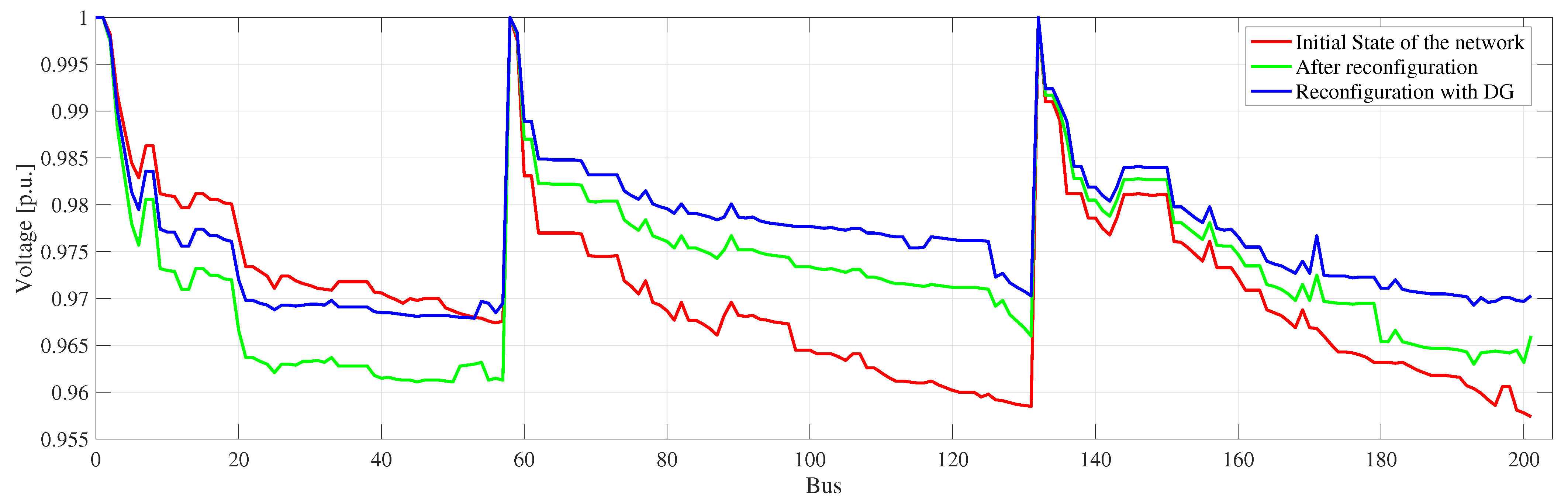
3.8. Case Study VI: 202-Bus Test System

This distribution system features 216 circuits with 201 tie switches and 15 normally open interconnection switches. The data of this system can be consulted in [66]. In its initial topology, switches 202, 203, 204, 205, 206, 207, 208, 209, 210, 211, 212, 213, 214, 215, and 216 are open. The nominal voltage is 13.8 kV, and the system must supply a load of $(27,571.56+j17,084.54)$ kVA. The initial value of active power losses (without reconfiguration) is 548.89 kW.

Table 8. Results for the 202-bus test system.

Case	Open Switches	DG Data				Power Losses	Reduction (%)	Vmin (p.u.)	$\mathbf{\Delta }\mathit{V}$	Time (s)
		Type	P (kW)	Q (kVAr)	Bus
I	202, 203, 204, 205, 206, 207, 208, 209, 210, 211, 212, 213, 214, 215, 216	–	–	–	–	548.89	–	0.9574	5.8695	–
II	12, 26, 43, 82, 118, 131, 133, 140, 168, 202, 203, 208, 212, 213, 214	–	–	–	–	511.17	6.87	0.9611	5.5111	71.44
III	12, 29, 44, 74, 82, 111, 118, 131,	1	996.76	327.62	42	336.55	38.68	0.9679	4.7119	745.36
	133, 140, 168, 184, 202, 212, 214	1	1000	328.58	50
		1	1000	328.58	53
		2	931.56	–	193
		2	701.34	–	201
		2	884.63	–	202

shows the open switches, active power losses, percentage of active power losses reduced, minimum voltage, and CPU time of the initial topology, and the optimal solutions found by the proposed mathematical model with and without DG units. In the case of optimal reconfiguration, the active power losses present a reduction of 6.87%, the minimum voltage improves from 0.9574 (base case) to 0.9611 p.u., and the CPU time is 71.44 s. On the other hand, the optimal reconfiguration considering DG proposes to install three Type 1 units at buses 42, 50, and 53 with a power of $(996.76+j327.62)$ kVA, $(1000+j328.68)$ kVA, and $(1000+j328.68)$ kVA, respectively. Furthermore, three Type 2 units at buses 193, 201, and 202 with an active power of $931.56$ kW, $701.34$ kW, and $884.63$ kW are installed. In this case, the active power losses present a reduction of 38.68%, the voltage deviation improves from 5.8695 (base case) to 4.7119, and the CPU time is 745.36 s. Note that the topology of the system is different with and without DG.

Figure 8 depicts the voltage profile of the initial state (base case) of the EDN, and the voltage profile after reconfiguration with and without DG. Note that the voltage profiles have been enhanced as a result of the optimal reconfiguration and with the reconfiguration considering DG.

4. Comparative Analysis of Results

To demonstrate the model’s applicability and efficacy, this section shows a comparative analysis of results with other papers reported in the specialized literature for both optimal reconfiguration alone and reconfiguration considering DG. In the case of reconfiguration with DG, only results of two distribution networks were found in the specialized literature. It is worth mentioning that the references that include DG within the DNR problem use a nonlinear model of the network and resort to metaheuristic techniques for its solution; also, a unity power factor is considered for all DG units.

The data regarding the maximum power generation and the number of units for the 33- and 69-bus test systems are taken from [59]. For the 33-bus test system, three DG units are considered, each one with 1279.6 kW of maximum capacity; furthermore, the maximum power to be injected by the DG units is limited to 2989.5 kW. For the 69-bus test system, three DG units are considered, each one with 1441.5 kW of maximum capacity; furthermore, the maximum power to be injected by the DG units is limited to 2469.1 kW.

Table 9. Comparative analysis of reconfiguration with distributed generation for the 33-bus test system.

Ref.	Type	Open Switches	Active Power of DG (kW)	Bus	Power Losses (kW)	Vmin (p.u.)
Proposed	Initial	33, 34, 35, 36, 37	–	–	202.67	0.9131
	R	7, 9, 14, 32, 37	–	–	139.54	0.9378
	R-DG	11, 28, 31, 33, 34	975.75	7	50.74	0.9723
			734.15	17
			1279.6	25
[59]	Initial	33, 34, 35, 36, 37	–	–	202.68	0.91309
	R	7, 9, 14, 32, 37	–	–	139.55	0.9378
	R-DG	11, 28, 31, 33, 34	956.9	7	50.72	0.9734
			723.0	17
			1279.6	25
[45]	Initial	33, 34, 35, 36, 37	–	–	202.67	0.9131
	R	7, 9, 14, 28, 37	–	–	139.98	0.9413
	R-DG	7, 11, 14, 28, 32	531.5	18	67.11	0.9713
			615.8	29
			536.7	32
[58]	Initial	33, 34, 35, 36, 37	–	–	202.67	0.9131
	R	7, 9, 14, 32, 37	–	–	139.5	–
	R-DG	7, 9, 14, 28, 31	345.0	13	57.35	–
			595.0	18
			1059.0	25
[51]	Initial	33, 34, 35, 36, 37	–	–	202.67	0.9131
	R	7, 9, 14, 28, 32	–	–	139.98	0.9412
	R-DG	7, 9, 13, 28, 32	412.78	15	64.97	0.9691
			1375.9	18
			1238.30	29
[69]	Initial	33, 34, 35, 36, 37	–	–	202.67	0.9131
	R	7, 9, 14, 28, 32	–	–	139.98	0.9412
	R-DG	10, 28, 31, 33, 34	723.7	7	57.987	0.9691
			742.9	17
			741.9	25

and

Table 10. Comparative analysis of reconfiguration with distributed generation for the 69-bus test system.

Ref.	Type	Open Switches	Active Power of DG (kW)	Bus	Power Losses (kW)	Vmin (p.u.)
Proposed	Initial	69, 70, 71, 72, 73	–	–	224.99	0.9092
	R	14, 55, 61, 69, 70	–	–	99.62	0.9427
	R-DG	14, 62, 63, 69, 70	549.6	11	35.72	0.9740
			1441.5	61
			477.9	65
[59]	Initial	69, 70, 71, 72, 73	–	–	224.89	0.9092
	R	14, 56, 61, 69, 70	–	–	98.57	0.9495
	R-DG	14, 56, 61, 69, 70	537.6	11	35.46	0.9813
			1441.5	61
			490.0	64
[45]	Initial	69, 70, 71, 72, 73	–	–	224.96	0.9092
	R	14, 56, 61, 69, 70	–	–	98.59	0.9495
	R-DG	13, 55, 63, 69, 70	1127.2	61	82.55	0.9796
			2750.0	62
			415.9	65
[58]	Initial	69, 70, 71, 72, 73	–	–	224.96	0.9092
	R	14, 58, 61, 69, 70	–	–	99.58	–
	R-DG	14, 58, 61, 69, 70	246.0	12	36.57	–
			1281.0	61
			472.0	64
[51]	Initial	69, 70, 71, 72, 73	–	–	224.97	0.9091
	R	12, 58, 61, 69, 70	–	–	98.79	0.9494
	R-DG	12, 57, 61, 69, 70	140.81	24	38.36	0.9777
			422.43	64

present a comparison of results with several references that include DG within the DNR problem. Three cases are considered: (i) the initial status of the system; (ii) the reconfiguration alone (labeled with an ‘R’), and (iii) the reconfiguration considering DG units (labeled as ‘R-DG’). On the other hand, the fourth column of Table 9 and Table 10 indicates the active power output of the DG units, followed by their location in parentheses. Note that the results regarding power losses are quite similar to those reported in [59] and better than those reported in other references. The difference in power losses is because we introduce a linear model, while in [59], a nonlinear modeling of the network is considered.

Table 11. Comparative analysis of the 16-bus test system.

Model	Open Switches	Power Losses (kW)	Time (s)
[3]	15, 17, 26	488.46	–
[4]	15, 17, 26	483.88	–
[70]	17, 19, 26	468.3	–
[71]	17, 19, 26	466.1	8
[72]	17, 19, 26	466.1	7.5
[73]	17, 19, 26	466.12	6
[68]	17, 19, 26	466.1	4.5
[17]	17, 19, 26	466.12	2.027
[18]	17, 19, 26	466.13	0.45
[19]	17, 19, 26	466.13	0.27
[8]	17, 19, 26	468.3	0.16
[13]	17, 19, 26	466.12	0.156
[33]	17, 19, 26	466.1	0.12

shows the optimal solution found by the proposed model with the 16-bus test system. Note that the reconfiguration found is the same as that previously published in the specialized literature; nonetheless, the solution is found in less computational time.

Table 12. Comparative analysis of the 33-bus test system.

Model	Open Switches	Power Losses (kW)	Time (s)
[71]	6, 9, 14, 32, 37	142.83	–
[74]	7, 9, 14, 32, 37	139.55	647.03
[8]	7, 9, 14, 32, 37	139.6	46
[75]	7, 9, 14, 32, 37	141.6	19.1
[28]	7, 10, 14, 36, 37	142.68	7.2
[5]	7, 10, 14, 32, 37	141.6	0.14
[73]	7, 9, 14, 32, 37	139.7	3
[76]	7, 9, 14, 31, 37	142	0.1
[77]	7, 9, 14, 32, 37	139.55	35.5
[7]	7, 9, 14, 32, 37	139.55	10.83
[24]	7, 9, 14, 32, 37	139.55	8.1
[25]	7, 9, 14, 32, 37	139.55	8
[16]	7, 9, 14, 32, 37	139.55	7.41
[78]	7, 9, 14, 32, 37	139.55	5.28
[70]	7, 9, 14, 32, 37	139.55	3.2
[6]	7, 9, 14, 32, 37	139.55	2.9
[33]	7, 9, 14, 32, 37	139.55	2.28
[79]	7, 9, 14, 32, 37	139.55	1.99
[80]	7, 9, 14, 32, 37	139.55	1.43
Proposed	7, 9, 14, 32, 37	139.55	0.46
[81]	7, 9, 14, 32, 37	139.55	0.41
[82]	7, 9, 14, 32, 37	139.55	0.11

presents the solutions found for the 33-bus test system with different methodologies. Note that the solution found is the same as the one reported in other papers; nonetheless, it is found in slightly higher time than some of the ones reported in the specialized literature.

Table 13. Comparative analysis of the 69-bus test system.

Model	Open Switches	Power Losses (kW)	Time (s)
[78]	13, 58, 61, 69, 90	99.72	–
[28]	14, 53, 61, 69, 70	103.29	–
[81]	14, 55, 61, 69, 70	99.62	–
[83]	14, 58, 61, 69, 70	99.62	–
[84]	14, 58, 61, 69, 70	99.62	–
[25]	14, 55, 61, 69, 70	99.62	150
[19]	14, 57, 61, 69, 70	99.62	20.2
[85]	14, 55, 61, 69, 70	99.62	12.5
[14]	14, 55, 61, 69, 70	99.62	8
[33]	14, 55, 61, 69, 70	99.62	6.17
Proposed	14, 55, 61, 69, 70	99.62	2.42

presents the solution found with the proposed approach for the 69-bus test system. In this case, the same power losses were obtained in less computational time.

Table 14. Comparative analysis of the 119-bus test system.

Model	Open Switches	Power Losses (kW)	Time (s)
[81]	24, 27, 35, 40, 43, 52, 59, 72, 75, 96, 98, 110, 123, 130, 131	869.70	–
[25]	24, 27, 35, 40, 43, 52, 59, 72, 75, 96, 98, 110, 123, 130, 131	869.70	18,000
[80]	24, 27, 35, 40, 43, 52, 59, 72, 75, 96, 98, 110, 123, 130, 131	869.70	1009
[86]	24, 27, 35, 40, 43, 52, 59, 72, 75, 96, 98, 110, 123, 130, 131	870.33	704.1
[85]	24, 27, 35, 40, 43, 52, 59, 72, 75, 96, 98, 110, 123, 130, 131	870.33	42.13
[8]	24, 27, 35, 40, 43, 52, 59, 72, 75, 96, 98, 110, 123, 130, 131	869.70	39.4
[28]	24, 35, 40, 43, 49, 51, 62, 73, 74, 77, 83, 110, 120, 126, 131	885.56	24.25
[24]	24, 27, 35, 40, 43, 52, 59, 72, 75, 96, 98, 110, 123, 130, 131	869.70	9.38
[6]	24, 27, 35, 40, 43, 52, 59, 72, 75, 96, 98, 110, 123, 130, 131	869.70	24.8
[33]	24, 27, 35, 40, 43, 52, 59, 72, 75, 96, 98, 110, 123, 130, 131	869.71	9.5
Proposed	24, 27, 35, 40, 43, 52, 59, 72, 75, 96, 98, 110, 123, 130, 131	869.71	3.82
[77]	24, 27, 35, 40, 43, 52, 59, 72, 75, 96, 98, 110, 123, 130, 131	869.71	2.8

shows the comparative results for the 119-bus test system. In this case, the topology and power losses found are the same as the ones already reported in the specialized literature. As regards computational time, the proposed solution presented the second-best time.

Table 15. Comparative analysis of the 136-bus test system.

Model	Open Switches	Power Losses (kW)	Time (s)
[78]	7, 38, 51, 55, 90, 97, 106, 118, 126, 137, 138, 141, 144, 145, 146, 147, 148, 150, 151, 152, 152, 155	282.77	–
[20]	7, 38, 51, 53, 90, 96, 106, 118, 126, 128, 137, 138, 141, 144, 145, 146, 147, 148, 150, 151, 156	280.40	–
[70]	7, 38, 51, 54, 84, 90, 96, 106, 118, 126, 128, 135, 137, 138, 141, 144, 145, 147, 148, 150, 151	280.38	1009
[8]	7, 38, 51, 54, 84, 90, 96, 106, 118, 126, 128, 135, 137, 138, 141, 144, 145, 147, 148, 150, 151	280.38	39.40
[7]	7, 35, 51, 90, 96, 106, 118, 126, 135, 137, 138, 141, 142, 144, 145, 146, 147, 148, 150, 151, 155	280.19	4473
[77]	7, 35, 51, 90, 96, 106, 118, 126, 135, 137, 138, 141, 142, 144, 145, 146, 147, 148, 150, 151, 155	280.19	1785
[33]	7, 35, 51, 90, 96, 106, 118, 126, 135, 137, 138, 141, 142, 144, 145, 146, 147, 148, 150, 151, 155	280.19	9.50
Proposed	7, 35, 51, 90, 96, 106, 118, 126, 135, 137, 138, 141, 142, 144, 145, 146, 147, 148, 150, 151, 155	280.19	7.07

and

Table 16. Comparative analysis of the 202-bus test system.

Model	Open Switches	Power Losses (kW)	Time (s)
[26]	29, 66, 74, 83, 111, 118, 125, 131, 135, 136, 140, 177, 199, 202, 208	537.1	49.98
[33]	12, 26, 43, 82, 118, 131, 133, 140, 168, 202, 203, 208, 212, 213, 214	511.19	948.64
Proposed	12, 26, 43, 82, 118, 131, 133, 140, 168, 202, 203, 208, 212, 213, 214	511.17	71.44

present a comparison of results for the 136-bus and 202-bus test systems. In both cases, the proposed model was able to find the global optimal solution in lower computational time.

5. Conclusions

The presence of small-scale generation units is becoming popular in modern EDNs. Therefore, studies regarding the operation and planning of EDNs must take into account the impact of DG units, indicating their best locations and the optimal topology that harvests their benefits and minimizes eventual negative impacts. This paper presented an MILP model for the optimal placement of DG and optimal reconfiguration of distribution networks. The main objectives of the proposed model are the minimization of active power losses and the improvement of the voltage profile. Due to its nature, the proposed model can be solved by commercially available solvers, guaranteeing global optimal solutions.

Several tests were performed on seven benchmark distribution systems with sizes ranging from 16 to 202 buses. In this sense, this paper aims to serve as a reference for future research since several types of test systems were used for comparative purposes. In all cases, the proposed model was able to obtain the global optimal solution reported in the specialized literature. In most cases, this solution was achieved with reduced computational time. As opposed to previous methods consulted in the specialized literature that have been tested in specific small-sized distribution networks, the proposed formulation proved to be effective for solving the simultaneous DNR and optimal placement of DG in real-sized distribution systems.

In the comparative analysis, it was found that when no DG units are considered, the proposed model is able to find the same results reported in the specialized literature but with less computational time. Furthermore, the inclusion of DG units, along with optimal reconfiguration, allows the model to find better solutions than those previously reported in the specialized literature. It is worth mentioning that the proposed model allows the consideration of several DG types.

The results obtained demonstrate that reconfiguration alone can improve the voltage profile and reduce power losses. Nonetheless, when the optimal DG placement and distribution network reconfiguration are solved concurrently, power losses are significantly reduced and voltage profile improvements are obtained.

References

1. Jaramillo Serna, J.J.; López-Lezama, J.M. Alternative Methodology to Calculate the Directional Characteristic Settings of Directional Overcurrent Relays in Transmission and Distribution Networks. Energies 2019, 12, 3779. [Google Scholar] [CrossRef] [Green Version]
2. Saldarriaga-Zuluaga, S.D.; López-Lezama, J.M.; Muñoz-Galeano, N. Optimal coordination of over-current relays in microgrids considering multiple characteristic curves. Alex. Eng. J. 2021, 60, 2093–2113. [Google Scholar] [CrossRef]
3. Civanlar, S.; Grainger, J.; Yin, H.; Lee, S. Distribution feeder reconfiguration for loss reduction. IEEE Trans. Power Deliv. 1988, 3, 1217–1223. [Google Scholar] [CrossRef]
4. Sarfi, R.; Salama, M.; Chikhani, A. Distribution system reconfiguration for loss reduction: An algorithm based on network partitioning theory. IEEE Trans. Power Syst. 1996, 11, 504–510. [Google Scholar] [CrossRef]
5. Shirmohammadi, D.; Hong, H. Reconfiguration of electric distribution networks for resistive line losses reduction. IEEE Trans. Power Deliv. 1989, 4, 1492–1498. [Google Scholar] [CrossRef]
6. Hijazi, H.; Thiébaux, S. Optimal distribution systems reconfiguration for radial and meshed grids. Int. J. Electr. Power Energy Syst. 2015, 72, 136–143. [Google Scholar] [CrossRef]
7. Lavorato, M.; Franco, J.F.; Rider, M.J.; Romero, R. Imposing Radiality Constraints in Distribution System Optimization Problems. IEEE Trans. Power Syst. 2012, 27, 172–180. [Google Scholar] [CrossRef]
8. Ahmadi, H.; Martí, J.R. Mathematical representation of radiality constraint in distribution system reconfiguration problem. Int. J. Electr. Power Energy Syst. 2015, 64, 293–299. [Google Scholar] [CrossRef]
9. Agudelo, L.; López-Lezama, J.M.; Muñoz-Galeano, N. Vulnerability assessment of power systems to intentional attacks using a specialized genetic algorithm. Dyna 2015, 82, 78–84. [Google Scholar] [CrossRef]
10. Pérez Posada, A.F.; Villegas, J.G.; López-Lezama, J.M. A Scatter Search Heuristic for the Optimal Location, Sizing and Contract Pricing of Distributed Generation in Electric Distribution Systems. Energies 2017, 10, 1449. [Google Scholar] [CrossRef] [Green Version]
11. Gerez, C.; Coelho Marques Costa, E.; Sguarezi Filho, A.J. Distribution Network Reconfiguration Considering Voltage and Current Unbalance Indexes and Variable Demand Solved through a Selective Bio-Inspired Metaheuristic. Energies 2022, 15, 1686. [Google Scholar] [CrossRef]
12. Gomes, F.; Carneiro, S.; Pereira, J.; Vinagre, M.; Garcia, P.; De Araujo, L. A New Distribution System Reconfiguration Approach Using Optimum Power Flow and Sensitivity Analysis for Loss Reduction. IEEE Trans. Power Syst. 2006, 21, 1616–1623. [Google Scholar] [CrossRef]
13. Sivanagaraju, S.; Rao, J.V.; Raju, P.S. Discrete Particle Swarm Optimization to Network Reconfiguration for Loss Reduction and Load Balancing. Electr. Power Components Syst. 2008, 36, 513–524. [Google Scholar] [CrossRef]
14. Abdelaziz, A.; Mohammed, F.; Mekhamer, S.; Badr, M. Distribution Systems Reconfiguration using a modified particle swarm optimization algorithm. Electr. Power Syst. Res. 2009, 79, 1521–1530. [Google Scholar] [CrossRef]
15. Yang, M.; Li, J.; Li, J.; Yuan, X.; Xu, J. Reconfiguration Strategy for DC Distribution Network Fault Recovery Based on Hybrid Particle Swarm Optimization. Energies 2021, 14, 7145. [Google Scholar] [CrossRef]
16. Zhu, J. Optimal reconfiguration of electrical distribution network using the refined genetic algorithm. Electr. Power Syst. Res. 2002, 62, 37–42. [Google Scholar] [CrossRef]
17. Sivanagaraju, S.; Srikanth, Y.; Babu, E.J. An Efficient Genetic Algorithm for Loss Minimum Distribution System Reconfiguration. Electr. Power Components Syst. 2006, 34, 249–258. [Google Scholar] [CrossRef]
18. Wang, C.; Gao, Y. Determination of Power Distribution Network Configuration Using Non-Revisiting Genetic Algorithm. IEEE Trans. Power Syst. 2013, 28, 3638–3648. [Google Scholar] [CrossRef]
19. Eldurssi, A.M.; O’Connell, R.M. A Fast Nondominated Sorting Guided Genetic Algorithm for Multi-Objective Power Distribution System Reconfiguration Problem. IEEE Trans. Power Syst. 2015, 30, 593–601. [Google Scholar] [CrossRef]
20. Guimarães, M.A.; Castro, C.A.; Romero, R. Distribution systems operation optimization through reconfiguration and capacitor allocation by a dedicated genetic algorithm. IET Gener. Transm. Distrib. 2010, 4, 1213. [Google Scholar] [CrossRef]
21. Guamán, A.; Valenzuela, A. Distribution Network Reconfiguration Applied to Multiple Faulty Branches Based on Spanning Tree and Genetic Algorithms. Energies 2021, 14, 6699. [Google Scholar] [CrossRef]
22. Amin, A.; Muhammad, M.; Mokhlis, H.; Franco, J.; Naidu, K.; Coo, L. Enhancement of Simultaneous Network Reconfiguration and DG Sizing via Hamming dataset approach and Firefly Algorithm. IET Gener. Transm. Distrib. 2019, 13, 5071–5082. [Google Scholar]
23. Gerez, C.; Silva, L.I.; Belati, E.A.; Sguarezi Filho, A.J.; Costa, E.C.M. Distribution Network Reconfiguration Using Selective Firefly Algorithm and a Load Flow Analysis Criterion for Reducing the Search Space. IEEE Access 2019, 7, 67874–67888. [Google Scholar] [CrossRef]
24. Zhang, D.; Fu, Z.; Zhang, L. An improved TS algorithm for loss-minimum reconfiguration in large-scale distribution systems. Electr. Power Syst. Res. 2007, 77, 685–694. [Google Scholar] [CrossRef]
25. Abdelaziz, A.; Mohamed, F.; Mekhamer, S.; Badr, M. Distribution system reconfiguration using a modified Tabu Search algorithm. Electr. Power Syst. Res. 2010, 80, 943–953. [Google Scholar] [CrossRef]
26. Guimarães, M.A.; Castro, C.A. Reconfiguration of Distribution Systems for Loss Reduction using Tabu Search. In Proceedings of the 15th Power System Computation Conference, Ghent, Belgium, 22–26 August 2005; pp. 1–6. [Google Scholar]
27. Saldarriaga-Zuluaga, S.D.; López-Lezama, J.M.; Muñoz-Galeano, N. Hybrid Harmony Search Algorithm Applied to the Optimal Coordination of Overcurrent Relays in Distribution Networks with Distributed Generation. Appl. Sci. 2021, 11, 9207. [Google Scholar] [CrossRef]
28. Srinivasa Rao, R.; Narasimham, S.V.L.; Ramalinga Raju, M.; Srinivasa Rao, A. Optimal Network Reconfiguration of Large-Scale Distribution System Using Harmony Search Algorithm. IEEE Trans. Power Syst. 2011, 26, 1080–1088. [Google Scholar] [CrossRef]
29. dos Santos, M.V.; Brigatto, G.A.; Garcés, L.P. Methodology of solution for the distribution network reconfiguration problem based on improved harmony search algorithm. IET Gener. Transm. Distrib. 2020, 14, 6526–6533. [Google Scholar] [CrossRef]
30. Tavakoli Ghazi Jahani, M.; Nazarian, P.; Safari, A.; Haghifam, M. Multi-objective optimization model for optimal reconfiguration of distribution networks with demand response services. Sustain. Cities Soc. 2019, 47, 101514. [Google Scholar] [CrossRef]
31. Haghighat, H.; Zeng, B. Distribution System Reconfiguration Under Uncertain Load and Renewable Generation. IEEE Trans. Power Syst. 2016, 31, 2666–2675. [Google Scholar] [CrossRef]
32. Borges, M.; Franco, J.; Rider, M.J. Optimal Reconfiguration of Electrical Distribution Systems Using Mathematical Programming. J. Control. Autom. Electr. Syst. 2014, 25, 103–111. [Google Scholar] [CrossRef] [Green Version]
33. Mahdavi, M.; Alhelou, H.H.; Hatziargyriou, N.D.; Al-Hinai, A. An Efficient Mathematical Model for Distribution System Reconfiguration Using AMPL. IEEE Access 2021, 9, 79961–79993. [Google Scholar] [CrossRef]
34. Mahmoud, K.; Yorino, N.; Ahmed, A. Optimal Distributed Generation Allocation in Distribution Systems for Loss Minimization. IEEE Trans. Power Syst. 2016, 31, 960–969. [Google Scholar] [CrossRef]
35. Akbari, M.A.; Aghaei, J.; Barani, M.; Niknam, T.; Ghavidel, S.; Farahmand, H.; Korpas, M.; Li, L. Convex Models for Optimal Utility-Based Distributed Generation Allocation in Radial Distribution Systems. IEEE Syst. J. 2018, 12, 3497–3508. [Google Scholar] [CrossRef]
36. Eid, A.; Kamel, S.; Korashy, A.; Khurshaid, T. An Enhanced Artificial Ecosystem-Based Optimization for Optimal Allocation of Multiple Distributed Generations. IEEE Access 2020, 8, 178493–178513. [Google Scholar] [CrossRef]
37. Sanjay, R.; Jayabarathi, T.; Raghunathan, T.; Ramesh, V.; Mithulananthan, N. Optimal Allocation of Distributed Generation Using Hybrid Grey Wolf Optimizer. IEEE Access 2017, 5, 14807–14818. [Google Scholar] [CrossRef]
38. Ali, M.H.; Kamel, S.; Hassan, M.H.; Tostado-Véliz, M.; Zawbaa, H.M. An improved wild horse optimization algorithm for reliability based optimal DG planning of radial distribution networks. Energy Rep. 2022, 8, 582–604. [Google Scholar] [CrossRef]
39. Ganguly, S.; Samajpati, D. Distributed Generation Allocation on Radial Distribution Networks Under Uncertainties of Load and Generation Using Genetic Algorithm. IEEE Trans. Sustain. Energy 2015, 6, 688–697. [Google Scholar] [CrossRef]
40. Ali, A.; Keerio, M.U.; Laghari, J.A. Optimal Site and Size of Distributed Generation Allocation in Radial Distribution Network Using Multi-objective Optimization. J. Mod. Power Syst. Clean Energy 2021, 9, 404–415. [Google Scholar] [CrossRef]
41. Elkadeem, M.R.; Abd Elaziz, M.; Ullah, Z.; Wang, S.; Sharshir, S.W. Optimal Planning of Renewable Energy-Integrated Distribution System Considering Uncertainties. IEEE Access 2019, 7, 164887–164907. [Google Scholar] [CrossRef]
42. Rueda-Medina, A.C.; Franco, J.F.; Rider, M.J.; Padilha-Feltrin, A.; Romero, R. A mixed-integer linear programming approach for optimal type, size and allocation of distributed generation in radial distribution systems. Electr. Power Syst. Res. 2013, 97, 133–143. [Google Scholar] [CrossRef]
43. Murthy, G.V.K.; Satyanarayana, S.; Rao, B.H. Artificial bee colony algorithm for distribution feeder reconfiguration with distributed generation. Int. J. Eng. Sci. Emerg. Technol. 2012, 3, 50–59. [Google Scholar]
44. Pavani, P.; Singh, S.N. Reconfiguration of radial distribution networks with distributed generation for reliability improvement and loss minimization. In Proceedings of the 2013 IEEE Power Energy Society General Meeting, Vancouver, BC, Canada, 21–25 July 2013; pp. 1–5. [Google Scholar] [CrossRef]
45. Imran, A.M.; Kowsalya, M.; Kothari, D. A novel integration technique for optimal network reconfiguration and distributed generation placement in power distribution networks. Int. J. Electr. Power Energy Syst. 2014, 63, 461–472. [Google Scholar] [CrossRef]
46. Sedighizadeh, M.; Esmaili, M.; Esmaeili, M. Application of the hybrid Big Bang-Big Crunch algorithm to optimal reconfiguration and distributed generation power allocation in distribution systems. Energy 2014, 76, 920–930. [Google Scholar] [CrossRef]
47. Muthukumar, K.; Jayalalitha, S. Integrated approach of network reconfiguration with distributed generation and shunt capacitors placement for power loss minimization in radial distribution networks. Appl. Soft Comput. 2017, 52, 1262–1284. [Google Scholar] [CrossRef]
48. Bayat, A.; Bagheri, A.; Noroozian, R. Optimal siting and sizing of distributed generation accompanied by reconfiguration of distribution networks for maximum loss reduction by using a new UVDA-based heuristic method. Int. J. Electr. Power Energy Syst. 2016, 77, 360–371. [Google Scholar] [CrossRef]
49. Aman, M.; Jasmon, G.; Mokhlis, H.; Bakar, A. Optimum Tie Switches Allocation and DG Placement Based On Maximization of System Loadability Using Discrete Artificial Bee Colony (DABC) Algorithm. IET Gener. Transm. Distrib. 2016, 10, 2277–2284. [Google Scholar] [CrossRef]
50. Rahiminejad, A.; Hosseinian, S.H.; Vahidi, B.; Shahrooyan, S. Simultaneous Distributed Generation Placement, Capacitor Placement, and Reconfiguration using a Modified Teaching-Learning-based Optimization Algorithm. Electr. Power Components Syst. 2016, 44, 1631–1644. [Google Scholar] [CrossRef]
51. Hormozi, M.A.; Jahromi, M.B.; Nasiri, G. Optimal Network Reconfiguration and Distributed Generation Placement in Distribution System Using a Hybrid Algorithm. Int. J. Energy Power Eng. 2016, 5, 163–170. [Google Scholar] [CrossRef] [Green Version]
52. Ahanch, M.; Asasi, M.S.; Amiri, M.S. A Grasshopper Optimization Algorithm to solve optimal distribution system reconfiguration and distributed generation placement problem. In Proceedings of the 2017 IEEE 4th International Conference on Knowledge-Based Engineering and Innovation (KBEI), Tehran, Iran, 22–22 December 2017; pp. 0659–0666. [Google Scholar] [CrossRef]
53. Abd El-salam, M.F.; Beshr, E.; Eteiba, M.B. A New Hybrid Technique for Minimizing Power Losses in a Distribution System by Optimal Sizing and Siting of Distributed Generators with Network Reconfiguration. Energies 2018, 11, 3351. [Google Scholar] [CrossRef] [Green Version]
54. Saleh, O.; Elshahed, M.; Elsayed, M. Enhancement of radial distribution network with distributed generation and system reconfiguration. J. Electr. Syst. 2018, 14, 36–50. [Google Scholar]
55. Ben Hamida, I.; Salah, S.; Faouzi, M.; Mimouni, M. Optimal network reconfiguration and renewable DG integration considering time sequence variation in load and DGs. Renew. Energy 2018, 121, 66–80. [Google Scholar] [CrossRef]
56. Sambaiah, K.S.; Jayabarathi, T. Optimal reconfiguration and renewable distributed generation allocation in electric distribution systems. Int. J. Ambient Energy 2021, 42, 1018–1031. [Google Scholar] [CrossRef]
57. Onlam, A.; Yodphet, D.; Chatthaworn, R.; Surawanitkun, C.; Siritaratiwat, A.; Khunkitti, P. Power Loss Minimization and Voltage Stability Improvement in Electrical Distribution System via Network Reconfiguration and Distributed Generation Placement Using Novel Adaptive Shuffled Frogs Leaping Algorithm. Energies 2019, 12, 553. [Google Scholar] [CrossRef] [Green Version]
58. Siahbalaee, J.; Rezanejad, N.; Gharehpetian, G.B. Reconfiguration and DG Sizing and Placement Using Improved Shuffled Frog Leaping Algorithm. Electr. Power Components Syst. 2019, 47, 1475–1488. [Google Scholar] [CrossRef]
59. Quadri, I.; Bhowmick, S. A hybrid technique for simultaneous network reconfiguration and optimal placement of distributed generation resources. Soft Comput. 2020, 24, 11315–11336. [Google Scholar] [CrossRef]
60. Nguyen, T.T.; Nguyen, T.T.; Nguyen, N.A.; Duong, T.L. A novel method based on coyote algorithm for simultaneous network reconfiguration and distribution generation placement. Ain Shams Eng. J. 2021, 12, 665–676. [Google Scholar] [CrossRef]
61. Raut, U.; Mishra, S. An improved sine–cosine algorithm for simultaneous network reconfiguration and DG allocation in power distribution systems. Appl. Soft Comput. 2020, 92, 106293. [Google Scholar] [CrossRef]
62. Shaheen, A.; Elsayed, A.; El-Sehiemy, R.A.; Abdelaziz, A.Y. Equilibrium optimization algorithm for network reconfiguration and distributed generation allocation in power systems. Appl. Soft Comput. 2021, 98, 106867. [Google Scholar] [CrossRef]
63. Franco, J.F.; Rider, M.J.; Lavorato, M.; Romero, R. A mixed-integer LP model for the optimal allocation of voltage regulators and capacitors in radial distribution systems. Int. J. Electr. Power Energy Syst. 2013, 48, 123–130. [Google Scholar] [CrossRef]
64. Gallego, L.A.; Franco, J.F.; Cordero, L.G. A fast-specialized point estimate method for the probabilistic optimal power flow in distribution systems with renewable distributed generation. Int. J. Electr. Power Energy Syst. 2021, 131, 107049. [Google Scholar] [CrossRef]
65. Cespedes, R.G. New method for the analysis of distribution networks. IEEE Trans. Power Deliv. 1990, 5, 391–396. [Google Scholar] [CrossRef]
66. Gallego, L.A.; López-Lezama, J.M.; Gómez, O. Data of the Electrical Distribution Systems for the Optimal Reconfiguration Used in This Paper. 2022. Available online: https://github.com/LuisGallego2019/ElectricalSystemsDataForReconfiguration (accessed on 21 March 2022).
67. Ramesh Babu, M.; Kumar, C.; Anitha, S. Simultaneous Reconfiguration and Optimal Capacitor Placement Using Adaptive Whale Optimization Algorithm for Radial Distribution System. J. Electr. Eng. Technol. 2020, 16, 181–190. [Google Scholar] [CrossRef]
68. Chiou, J.P.; Chang, C.F.; Su, C.T. Variable scaling hybrid differential evolution for solving network reconfiguration of distribution systems. IEEE Trans. Power Syst. 2005, 20, 668–674. [Google Scholar] [CrossRef]
69. Ben Hamida, I.; Salah, S.; Faouzi, M.; Mimouni, M. Optimal integration of distributed generations with network reconfiguration using a Pareto algorithm. Int. J. Renew. Energy Res. 2018, 8, 345–356. [Google Scholar]
70. Ahmadi, H.; Martí, J.R. Distribution System Optimization Based on a Linear Power-Flow Formulation. IEEE Trans. Power Deliv. 2015, 30, 25–33. [Google Scholar] [CrossRef]
71. Kashem, M.; Jasmon, G.; Ganapathy, V. A new approach of distribution system reconfiguration for loss minimization. Int. J. Electr. Power Energy Syst. 2000, 22, 269–276. [Google Scholar] [CrossRef]
72. Su, C.T.; Lee, C.S. Feeder reconfiguration and capacitor setting for loss reduction of distribution systems. Electr. Power Syst. Res. 2001, 58, 97–102. [Google Scholar] [CrossRef]
73. Chang, H.C.; Kuo, C.C. Network reconfiguration in distribution systems using simulated annealing. Electr. Power Syst. Res. 1994, 29, 227–238. [Google Scholar] [CrossRef]
74. Llorens-Iborra, F.; Riquelme-Santos, J.; Romero-Ramos, E. Mixed-integer linear programming model for solving reconfiguration problems in large-scale distribution systems. Electr. Power Syst. Res. 2012, 88, 137–145. [Google Scholar] [CrossRef]
75. Nara, K.; Shiose, A.; Kitagawa, M.; Ishihara, T. Implementation of genetic algorithm for distribution systems loss minimum re-configuration. IEEE Trans. Power Syst. 1992, 7, 1044–1051. [Google Scholar] [CrossRef]
76. Schmidt, H.; Ida, N.; Kagan, N.; Guaraldo, J. Fast reconfiguration of distribution systems considering loss minimization. IEEE Trans. Power Syst. 2005, 20, 1311–1319. [Google Scholar] [CrossRef]
77. Ahmadi, H.; Martı´, J.R. Linear Current Flow Equations With Application to Distribution Systems Reconfiguration. IEEE Trans. Power Syst. 2015, 30, 2073–2080. [Google Scholar] [CrossRef]
78. Ferdavani, A.; Mohd Zin, A.; Khairuddin, A.; Naeini, M. Reconfiguration of distribution system through two minimum-current neighbor-chain updating methods. Gener. Transm. Distrib. IET 2013, 7, 1492–1497. [Google Scholar] [CrossRef]
79. McDermott, T.; Drezga, I.; Broadwater, R. A heuristic nonlinear constructive method for distribution system reconfiguration. IEEE Trans. Power Syst. 1999, 14, 478–483. [Google Scholar] [CrossRef]
80. Taylor, J.A.; Hover, F.S. Convex Models of Distribution System Reconfiguration. IEEE Trans. Power Syst. 2012, 27, 1407–1413. [Google Scholar] [CrossRef]
81. Raju, G.K.V.; Bijwe, P.R. An Efficient Algorithm for Minimum Loss Reconfiguration of Distribution System Based on Sensitivity and Heuristics. IEEE Trans. Power Syst. 2008, 23, 1280–1287. [Google Scholar] [CrossRef]
82. Khodr, H.M.; Martinez-Crespo, J.; Matos, M.A.; Pereira, J. Distribution Systems Reconfiguration Based on OPF Using Benders Decomposition. IEEE Trans. Power Deliv. 2009, 24, 2166–2176. [Google Scholar] [CrossRef]
83. Kashem, M.; Ganapathy, V.; Jasmon, G. A geometrical approach for network reconfiguration based loss minimization in distribution systems. Int. J. Electr. Power Energy Syst. 2001, 23, 295–304. [Google Scholar] [CrossRef]
84. Arun, M.; Aravindhababu, P. A new reconfiguration scheme for voltage stability enhancement of radial distribution systems. Energy Convers. Manag. 2009, 50, 2148–2151. [Google Scholar] [CrossRef]
85. Khorshid-Ghazani, B.; Seyedi, H.; Mohammadi-ivatloo, B.; Zare, K.; Shargh, S. Reconfiguration of distribution networks considering coordination of the protective devices. IET Gener. Transm. Distrib. 2017, 11, 82–92. [Google Scholar] [CrossRef]
86. de Oliveira, L.W.; de Oliveira, E.J.; Gomes, F.V.; Silva, I.C.; Marcato, A.L.; Resende, P.V. Artificial Immune Systems applied to the reconfiguration of electrical power distribution networks for energy loss minimization. Int. J. Electr. Power Energy Syst. 2014, 56, 64–74. [Google Scholar] [CrossRef]
Figure 1. Illustrative example of circuits and loads in an EDN.
Energies 15 03063 g001
Figure 2. Voltage profile of the 16-bus test system.
Energies 15 03063 g002
Figure 3. Voltage profile of the 33-bus test system.
Energies 15 03063 g003
Figure 4. Voltage profile of the 69-bus test system.
Energies 15 03063 g004
Figure 5. Voltage profile of the 84-bus test system.
Energies 15 03063 g005
Figure 6. Voltage profile of the 119-bus test system.
Energies 15 03063 g006
Figure 7. Voltage profile of the 136-bus test system.
Energies 15 03063 g007
Figure 8. Voltage profile of the 202-bus test system.
Energies 15 03063 g008