Multiperiod Portfolio of Energy Purchasing Strategies including Climate Scenarios

Abstract

Because electricity retailers must ensure that energy supply matches end-user demand, electricity that is not traded through bilateral contracts is typically traded in power exchanges which are subject to great price volatility. In Colombia, the spot price is a reflection of climate variability because approximately 70% of the country’s electricity is generated by large hydropower stations. In this study, we forecast 2018′s prices and calculated its corresponding purchase margins using the 2015 to 2017 bilateral contract prices for electricity plus power exchange price information and climate information. Our forecasts included climate uncertainty and evaluated two multi-period portfolio methods for deciding among three purchasing strategies: bilateral contracts in the regulated market, bilateral contracts in the non-regulated markets, and purchases in the power exchange. The results indicate that retailers should follow a middle course that is neither conservative nor risky. Creation of portfolios independent of the multi-period method can balance purchases through bilateral contracts and in the power exchange in a way that considers climatic uncertainty. This type of balanced portfolio could control medium-term risks of price volatility and result in good levels of purchase margins.

1. Introduction

In enterprise risk management, risk is defined as any event or action that may adversely affect an organization’s ability to achieve its objectives and execute its strategies [1], where two types of risk have been among the most studied: variability risk and vulnerability risk [2]. Variability risk is the difference between the actual and expected returns on an investment [3,4,5] and vulnerability risk includes default and bankruptcy risks [6,7]. In particular, variability risk management involves optimizing portfolios to allocate capital in a way that reduces the exposure of assets to risk [8,9]. One optimization method that has been applied with great success in the energy sector [10] is the establishment of efficient portfolios based on the determination of the efficient minimum portfolio risk for a given return [11,12].

Portfolio management in the electricity sector has been applied to all activities in the production chain but has mainly focused on the wholesale side of the electricity market. Only a few works have explored the retail side [9,13]. In particular, electricity retailers have to match supply with varying consumer demand [9] which causes their decisions to focus on the creation of portfolios based on purchasing strategies that mix power exchange purchases with longer-term purchases through bilateral contracts and can include self-generating capacity [14,15,16,17]. Within this framework, strategies can include forward contracts, call options, and interruptible contracts [9]. Recent research on optimal portfolios for retailers has mainly used the mean-variance approach [15,16,18] and stochastic optimization [9,13,19] with various measures such as value at risk (VaR), and conditional value at risk (CVaR) [9,14,17,19,20]. Some studies have proposed static models with no analysis of time [16,19,21] whereas others use dynamic models with timelines ranging from hourly portfolios [14], to one week [15], and on to medium-term planning of four weeks [18,22] to two months [9,13,17].

This paper focuses on the management of the variability risks faced by electricity retailers due to price uncertainty, exploring new issues in portfolio management for energy retailers that permit making two contributions. First, we considered weather uncertainty as a factor that increases the risks derived from energy price variability. Prior to our review, this key factor in Colombian energy markets had not been analyzed by other studies. Second, we developed a multi-period approach to portfolio construction that uses the “Buy and Hold” and the “Fixed-Mix” strategies, for electricity retailers in the Colombian context. Each strategy was considered within the climatic scenarios generated for price forecasting. We used the portfolio theory proposed by Markowitz [11], and we considered a planning scenario of one year, divided into quarters, for both multi-period strategies [23]. We showed that through providing short-term purchasing strategies this model will help energy retailers in countries such as Colombia hedge risks due to uncertain supply caused by weather phenomena, such as El Niño.

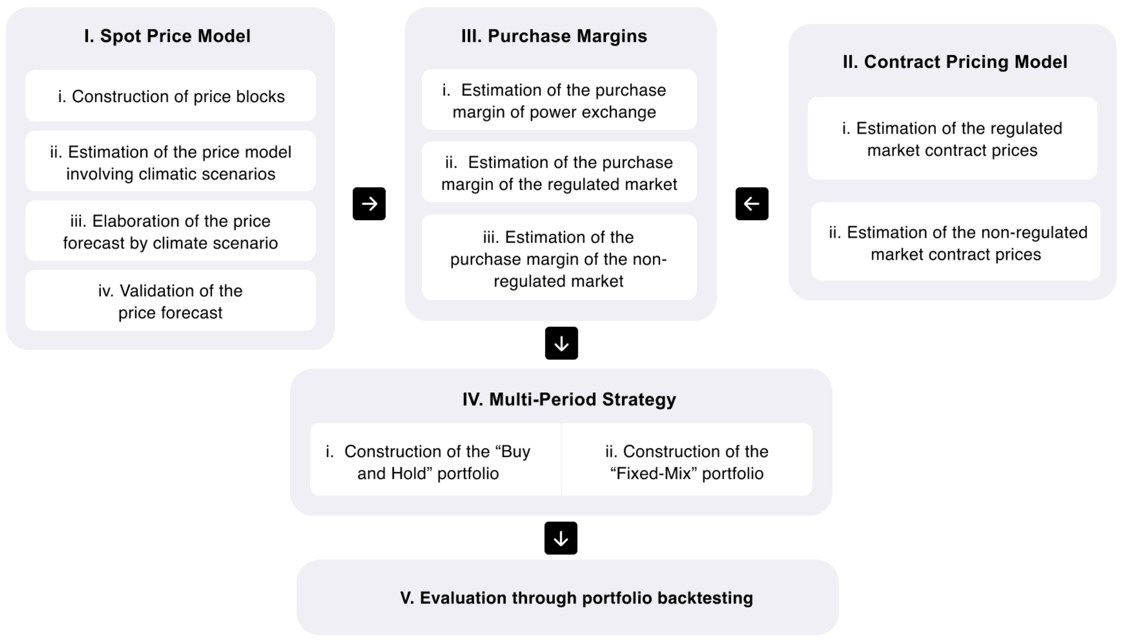
This document is divided into five sections. This introduction briefly describes the context and introduces electricity market risk management. The second part reviews the literature related to the Colombian electricity market, allocation strategies used to create optimal multi-period energy purchasing portfolios, and methodologies for forecasting electricity periods. The third section describes the methodology used to solve the problem. It contains our power exchange price model that includes weather variables and contracts, which can be used to find retailers’ margins. It is followed by the formulation of multi-period portfolios using the two most common allocation strategies. Finally, the relevant results and conclusions of the investigation are analyzed.

2. Literature Review

This section contains three parts: a description of the Colombian energy market, an explanation of general portfolio theory, and a multi-period portfolio using several strategies, which ends with an explanation of pricing models and the effects of weather conditions.

2.1. Power Sector in Colombia

Colombia is in the northwest corner of South America. Water is particularly important for generating electricity: large hydropower stations account for approximately 70% of the total production [24]. The rest is produced by coal and natural-gas-fired thermal plants. The 2020 energy demand of the Colombian grid, known as SIN for its Spanish acronym (Sistema Interconectado Nacional—National Interconnected System) was 70.422 GWh. This was a reduction of 2.60% from 2019 due to the effects of the COVID-19-induced economic downturn [25].

The Colombian power sector’s production chain includes generating companies, transmission companies, distributors, and retailers. Its market structure is based on competition among generators and in retail activities as established by Laws 142 and 143 of 1994 [26]. Large consumers and retailers may buy electricity directly from generators through medium-to-long-term contracts and/or in the short-term market.

According to XM S.A E.S.P., Colombia currently has 136 retailers who operate within a regulated market and a non-regulated market. The regulated market covers industrial, commercial, and residential consumers whose individual energy demands are less than 55 MWh. The prices of energy in this market are subject to a rate formula established by CREG (the Comisión de Regulación de Energía y Gas—Colombian Commission for the Regulation of Energy and Gas). Consumers are classified as residential or non-residential. About 98% of the consumers are in the regulated market, and all regulated consumers are supplied regardless of their consumption. On the other hand, industry and all other large-scale consumers can participate voluntarily in the non-regulated market. Large-scale consumers are defined as those whose average monthly power demand is greater than 0.1 MW or whose maximum average demand over the previous six months has been greater than 55 MWh/month [27]. Retailers and large consumers’ agents are free to negotiate energy prices directly through bilateral contracts.

Electricity purchase prices are among retailers’ biggest concerns: the lower the price, the greater their profit margins. These prices can be affected by multiple factors including weather, changes in fiscal policies and legal requirements, OPEC decisions, and transportation problems [28]. Since Colombia is highly dependent on water supplies for hydroelectric generation, during water shortages thermal power plants set high spot prices. In contrast, the normally rainy conditions allow hydropower plants to lead the energy exchange, and the spot prices are low. Under neutral rainy conditions, spot prices are lower than contract prices, independent of whether the target market is regulated or non-regulated. Figure 1 shows the average prices of the three markets: spot, regulated, and non-regulated, for the period 2015–2020. The average monthly spot price refers to the average of the hourly spot prices weighted by the energy traded on the stock exchange during each month. The monthly average price of the regulated market is calculated considering the average price, weighted by the voltage level, of the contracts destined for the regulated market. The average monthly price of the non-regulated market is calculated considering the average price of the monthly contracts registered in the ASIC, named using its Spanish acronym (Administrador del Sistema de Intercambios Comerciales—Administrator of the Commercial Exchange System), for the non-regulated market, weighted by voltage level. The source of this information was XM S.A. E.S.P. This figure also includes the Oceanic El Niño Index (ONI), which is calculated by The National Oceanic and Atmospheric Administration (NOAA). ONI allows the identification of warm (El Niño) and cold (La Niña) events in the tropical Pacific Ocean. The El Niño phenomenon is represented by ONI’s values greater than 0.5 and the La Niña phenomenon by ONI’s values of less than −0.5.

It can be seen that spot price volatility is greater than contract price volatility. In 2015, due to that year’s powerful El Niño, spot prices increased by up to 400% over contract prices, surpassing prices of USD 0.36/kWh. The positive relationship between the ONI index and spot prices is evidenced in the observation of higher ONI values occurring when higher spot prices occur. In contrast, in periods where ONI’s values are low, the spot prices reach the minimum level compared with contract prices.

2.2. Portfolio Theory

The mean-variance optimization proposed by Markowitz [11,12] produces an efficient frontier comprising a set of efficient portfolios. The efficient frontier is the set of “mean-variance choices” of the set of possibilities wherein returns are maximized given the risk of a portfolio, and no other investment opportunity offers a higher average return.

The literature includes a number of variations of objective functions including maximization of diversification [16], inclusion of Var and CVar models [14], and various risk preferences [17,29,30]. Although previous studies have focused on single-period portfolio decisions, recently there have been more studies that have included multiperiod analysis [31].

The formulation of the efficient mean-variance frontier is as follows:

$$\begin{gathered} \mathrm{Max} {\mathit{w}}^{\mathit{T}}{\mathit{\mu }}_r \\ \mathrm{s}.\mathrm{t}.{\mathit{w}}^{\mathit{T}}\mathit{\Sigma }\mathit{w}=k \\ {w}_i\ge 0, {\sum }_{i=1}^n{w}_i=1 \end{gathered}$$

(1)

where $\mathit{w}$ is a vector with the positive weights of n stocks. Their sum is equal to 1. ${\mathbf{\mu }}_r$ represents the vector of expected returns of the stocks that make up the portfolio. $\mathit{\Sigma }$ represents the matrix of variances and covariances on returns on assets, and $k$ represents a given value of risk.

2.2.1. Multi-Period Portfolio

The multi-period model considers the most general case in which an investor makes a sequence of decisions, each of which can affect subsequent decisions [23]. The model’s aim is to find an allocation decision in each period that includes a future set of changing factors that include availability of assets, risk-return characteristics, the remaining investment horizon, and eventual transaction costs, among others [32].

The multi-period model has been used previously in portfolio studies to manage risks [33,34,35]. Li and Ng state that portfolio selection from various periods has been dominated by the results of maximizing expected utility functions for final wealth [36]. However, they consider that there is no analytical or efficient numerical method to formulate the optimal portfolio policy over various periods.

Later, Collomb analyzed different asset allocation strategies for both a single period and a multi-period portfolio. In the multiple-period analyses, this author presented three types of allocation strategies: the Buy and Hold strategy, the Fixed-Mix strategy, and Stochastic optimization [23]. As its name suggests, the Buy and Hold strategy does not rebalance portfolio weights once the initial allocation decision has been made [37]. In the Fixed-Mix strategy, the allocation of weights for each purchasing strategy changes for each period, i.e., the weights are rebalanced in each period [38,39]. Finally, Stochastic optimization is based on scenarios [40] such as those proposed by Kettunen, Salo, and Bunn [29] and Safdarian, Fotuhi-Firuzabad, and Lehtonen [41]. A portfolio that changes each period is created in order to allow the generation of random electricity-price and customer-demand scenarios. This study delves into the two first strategies.

2.2.2. Buy and Hold and Fixed-Mix Models

In the Buy and Hold strategy a decision to purchase a passive investment is made at the beginning of each period and is maintained until the end of the planning horizon. To construct the portfolio, the mean-variance optimization model proposed by Markowitz [11,12] follows the mathematical formulation in Equation (1).

The “Fixed-Mix” portfolio strategy allocates weights for each energy purchasing strategy. The weights change each period, so the portfolio is rebalanced in each period. Following Collomb, the optimization model is defined using the mean-variance criterion [23]. In the first period, we have the optimization model proposed in Equation (1), and the weights are equal to $W_{t-1}$, which denotes the wealth that the investor begins with. is the initial budget. The mathematical formulation for the first period is:

$$\begin{gathered} \mathrm{Max}{\mathit{w}}^{\mathit{T}}{\mathit{\mu }}_r=R_t \\ \mathrm{s}.\mathrm{t}.{\mathit{w}}^{\mathit{T}}\mathit{\Sigma }\mathit{w}=k \\ {w}_i\ge 0, {\sum }_{i=1}^n{w}_{i1}=1 \end{gathered}$$

(2)

where $w$ is the vector of the positive weights of “n” stocks at time t = 1, and its sum is equal to 1. ${\mathbf{\mu }}_r$ represents the vector of the expected returns of the stocks that make up the portfolio, $R_t$ is the return at time t, $\mathit{\Sigma }$ represents the matrix of variances and covariances on the returns of the assets, and $k$ represents a given risk.

In subsequent periods, when t is greater than 1, previous earnings are used to rebalance the portfolios, following this formulation:

$$\begin{gathered} \mathrm{Max} {\mathit{w}}^{\mathit{T}}{\mathit{\mu }}_r =R_t \\ \mathrm{s}.\mathrm{t}.{\mathit{w}}^{\mathit{T}}\mathit{\Sigma }\mathit{w}=k \\ {\sum }_{i=1}^n{w}_{it}=(R_{t-1}+R_t) / R_{t-1} \\ {w}_i\ge 0,t>1 \end{gathered}$$

(3)

The final return for the total period Z is given by:

$$R_F={\prod }_{t=2}^Z\left(1+R_t\right)-1$$

(4)

2.3. Pricing Models and Effects of Weather Conditions

Given that retailers can buy energy either through bilateral contracts or directly on the power exchange at the spot price, any model should include price forecasts for both. The methodologies that have commonly been used to model the spot prices are variations of the Markov regime [42,43,44,45], GARCH models [42,46], the ARIMA-GARCH model [47], neural networks [48], and stochastic processes [49].

Generalized AutoRegressive Conditional Heteroscedasticity (GARCH) models have been fundamental for the valuation of derivatives. Initially proposed by Bollerslev and Engle, their main feature is conditional heteroscedasticity [50,51]. In other words, their structures of conditional variance depend not only on past errors but also on past conditional variance. Contreras et al. and Contreras and Rodriguez have proposed a methodology for modeling monthly Colombian electricity prices using an ARIMA (autoregressive integrated moving average)–GARCH model [16,47]. We have revised the method proposed by those authors to introduce climate scenarios into the pricing model.

For estimation of the ARIMA–GARCH model, following the notation of Garcia, Contreras, VanAkkeren, and Garcia [42], ARIMA (p, q)–GARCH (p, q) can be expressed as:

$$\left(1-{\sum }_{i=1}^p{\varphi }_i{L}^i\right)P_t=c+\left(1+{\sum }_{i=1}^p{\theta }_i{L}^i\right){\epsilon }_t$$

(5)

where $P_t$ denotes the price of electricity at time t, and L represents the delay operator that acts on the variable $y_t$ thus: $L(y_t)=y_t-1$. The ${\varphi }_i$ terms denote the self-regressive p-parameters, c is a constant term, the ${\theta }_i$ terms represent the moving average q-parameter, and ${\epsilon }_t$ refers to the error at time t. The square of the error term is given by:

$${\epsilon }_t^2={\nu }_t^2{\sigma }_t$$

(6)

where ${\nu }_t^2$ represents normally distributed white noise, for example, ${\nu }_t^2~N\left(0.1\right)$, and t is the time-dependent variance term expressed as:

$${\sigma }_t=c+{\sum }_{i=1}^p{\alpha }_i{\sigma }_{t-1}+{\sum }_{i=1}^q{\beta }_i{\epsilon }_{t-1}^2$$

(7)

where c is a constant term, the ${\alpha }_i$ terms represent the P lagged variance parameters, and the $\beta \prime$ terms denote the Q lagged error parameters.

The maximum likelihood method is used to calculate the parameters of both the model for the mean defined in Equation (5) and for the variance defined in Equation (7). In this way, unbiased and efficient estimators are produced.

Predicting weather events is difficult, but several institutes continuously monitor climate change, and pay special attention to prediction of El Niño. This is the case with ONI. The ONI is calculated as the three-month moving average of sea surface temperature anomalies for the region. The NINO 3.4 index is the forecast of the International Institute for Climate and Society Research (IRI) at Columbia University. It is one of several El Niño/Southern Oscillation (ENSO) indicators based on sea surface temperatures. Using this forecast, the IRI constructs probabilities of the occurrence of El Niño and La Niña.

Table 1. Probabilities for the ENSO forecast in the middle of the month from the IRI.

Period	La Niña	Neutral	El Niño
DJF 2018	83%	17%	0%
JFM 2018	72%	28%	0%
FMA 2018	56%	44%	0%
MAM 2018	36%	64%	0%
AMJ 2018	22%	74%	4%
MJJ 2018	19%	65%	16%
JJA 2018	18%	54%	28%
JAS 2018	16%	48%	36%
ASO 2018	17%	42%	41%
SON 2018	19%	41%	40%
OND 2018	20%	36%	44%
NDJ 2018	18%	34%	48%

Source: International Research Institute for Climate and Society [52].

shows the forecasts made in December 2017 for nine overlapping periods of three months each.

These probabilities show how for the first quarter of 2018 the probability of the occurrence of the La Niña phenomenon was greater compared with the other two climatic states, whereas in the middle of the year neutral conditions were expected, and at the end of the year the probability of the occurrence of the phenomenon of El Niño increased.

3. Methodology

This section’s two parts include the methodological steps followed to construct and evaluate the energy purchasing portfolio model involving climate scenarios plus a description of the data and information sources.

3.1. Portfolio Construction and Evaluation

We propose the four steps below for constructing retailer portfolios that minimize the risks of price volatility. In addition, we propose a fifth step for portfolio evaluation. Figure 2 shows the relationships among the 5 steps.

• Spot Price Model
  The spot price model involves four stages.
  • Construction of price blocks

In Colombia, the hourly volatility of spot prices is low, and hourly electricity prices often do not change for several hours. Consequently, it is necessary to group identical hourly prices into time blocks to better reflect the behavior of a series [47]. Following Contreras and Rodriguez [47], we have used cluster analysis to group hours based on the Euclidean distance calculation.

• Estimation of the price model involving climatic scenarios

Since part of the great volatility of prices on the Colombian power exchange is explained by climatic changes, we decided to elaborate several price models considering climatic phenomenon. In

Table 2. The ONI (Oceanic El Niño Index) three-month moving average.

Year	DJF	JFM	FMA	MAM	AMJ	MJJ	JJA	JAS	ASO	SON	OND	NDJ
2015	0.6	0.6	0.6	0.8	1	1.2	1.5	1.8	2.1	2.4	2.5	2.6
2016	2.5	2.2	1.7	1	0.5	0	−0.3	−0.6	−0.7	−0.7	−0.7	−0.6
2017	−0.3	−0.1	0.1	0.3	0.4	0.4	0.2	−0.1	−0.4	−0.7	−0.9	−1
2018	−0.9	−0.8	−0.6	−0.4	−0.1	0.1	0.1	0.2	0.4	0.7	0.9	0.8

Source: National Oceanic and Atmospheric Administration [53].

the ONI is presented as the moving average temperature anomaly of three consecutive months from December-January-February (DJF) of 2015 to November-December-January (NDJ) of 2018.

The period from 2015 to 2017 was reclassified as follows: the weak period of El Niño (months with ONI between 0.5 and 1.5), the strong period of El Niño (months with ONI greater than 1.5), and the La Niña phenomenon (months with ONI less than −0.5). An ARIMA–GARCH model was elaborated for each of these periods using the AIC as the fit criterion. This allowed us to distinguish among the set of possible models. Below, we explain the three models for each of the climatic scenarios: El Niño, La Niña, and neutral patterns in the Pacific Ocean that can affect weather worldwide.

• Elaboration of the price forecast by climate scenario

Retailers’ electricity purchase decisions are made at the beginning of the year, but the weather can vary within any given quarter, so prices can also vary within and by quarters. Three climatic scenarios can occur in any particular quarter: El Niño, La Niña, or neutral weather. The probabilities of occurrence of each scenario were taken from the International Institute for Climate and Society Research (IRI) at Columbia University. Its forecast is the NINO3.4 index, one of several El Niño/Southern Oscillation (ENSO) indicators based on ocean surface temperatures. Based on this forecast, we constructed probabilities of the occurrence of El Niño and La Niña.

A probability tree was constructed (Figure 3) with a total of 81 scenarios calculated as the Cartesian product of the three climate scenarios and the four quarters of the year. Figure 3 shows a succession of purchase decisions. The first decision is made at the initial stage. In the first quarter of 2018, the probability of La Niña occurring is P1, which is represented by a circle. The neutral weather scenario is represented by a square, and its probability of occurring is P2. The occurrence of the El Niño phenomenon is represented by a rhombus, and its probability of occurrence is P3. At the end of the four quarters, the sum of the probability of the 81 scenarios will be 1.

• Validation of the price forecast

To validate the capacity of the GARCH model that includes climate uncertainty to predict energy prices, we calculated the forecast error per hourly block by:

$$Forecast Error=\left(\frac{P_{t }-\widehat{P_t}}{P_t}\right)\times 100$$

(8)

where $P_{t }$ and $\widehat{P_t}$ refer to actual and forecast hourly block prices.

The daily average errors are calculated as the average of the forecast errors of the four hourly blocks. The monthly average errors were calculated as the average of the daily average errors, and the annual average error was calculated as the average of the monthly average errors. A similar study has allowed models that do not exceed 15% of the monthly average error [47].

II.

Contract Pricing Model

Bilateral contracts can be negotiated in either the regulated or non-regulated market. Following Contreras and Rodriguez [47], growth rates for bilateral contracts were estimated. The choice of this method was based on the fact that contractual prices in the regulated and non-regulated markets present trends which are maintained in the short term. This behavior occurs for both purchase and sale prices. The two stages of this step are the estimation of regulated market contract prices and estimation of non-regulated market contract prices.

III.

Purchase Margins

Computation of purchase margins (PM) (retailers’ profit margins) for each strategy requires purchase and sale prices. The mathematical formula is presented below:

$$P{M}_{jt}=\frac{\left(S{P}_{jt }-P{P}_{jt}\right)}{P{P}_{jt}}$$

(9)

where $P{M}_{jt}$ represents the purchase margin of strategy j at time t, $P{P}_{jt}$ refers to the purchase price of strategy j at time t, and $S{P}_{jt }$ refers to the sale price of strategy j at time t. In this step, three estimations of purchase margins must be made, one each for transactions on the power exchange, the regulated market, and the non-regulated market.

IV.

Multi-period strategy

The “Buy and Hold” and “Fixed-Mix” multi-period strategies were used to find solutions for retailers’ electricity purchases.

At the beginning of the period in the “Buy and Hold” strategy, the retailer decides to make a passive purchase investment. This investment is held until the end of the planning horizon. Mean-variance portfolios were calculated using the purchase margin forecasts for all of 2018 and the optimization model proposed in Equation (1). The decision is made in the first quarter of the year and is held for the subsequent three quarters.

The “Fixed-Mix” portfolio strategy allocates weights for each purchasing strategy change in each period. In other words, weights are rebalanced in each period. Using Equation (2) to Equation (4), a portfolio can be found for each quarter.

V.

Portfolio Performance Evaluation

Portfolio performance evaluation for each strategy was done using backtesting.

• Evaluation through portfolio backtesting

Portfolio backtesting is a powerful method to evaluate how well a strategy or model would have done ex-post. This method uses several tests to evaluate portfolio performance and then compares the results. We used four performance criteria: maximum drawdown, the Sharpe ratio, the Sterling ratio, and the Omega ratio.

Maximum drawdown (MDD) assesses the relative riskiness of a portfolio strategy compared with other strategies over a specified time period [54]. MDD, the maximum fall in the value of the investment, can be represented by the minimum percentage difference between the actual return and the highest return presented with respect to the highest return in period Z. We took the quotients between value 1, the difference between each daily return and the highest return in the analyzed period, and value 2, the highest return in the analyzed period, and then we chose the minimum quotient between the negative values obtained. The formula for maximum drawdown that we used is

$$\mathrm{MDD}=\left|Min \left[\frac{R_t-HR}{HR}\right]\right|$$

(10)

where $R_t$ represents the return in the period t and $HR$ represents the highest return obtained from $t=1$ to $t=Z$.

The Sharpe ratio measures the performance of the portfolio. It is calculated as the quotient of the portfolio return and the standard deviation of the portfolio. This criterion represents the additional amount of return that an investor receives per unit of increase in risk [55]. The formula for the Sharpe ratio is:

$$\mathrm{Sharpe}\mathrm{ratio}=\frac{\mathrm{Portfolio}\mathrm{return}}{\mathrm{Standard}\mathrm{deviation}}$$

(11)

The Sterling ratio measures the risk-adjusted return of an investment portfolio. There are several commonly used variations of the Sterling ratio, but all measure returns over average drawdown in contrast to the more commonly used maximum drawdown. Any investment with a ratio greater than 1.0 has a better than average risk-return tradeoff, since the Sterling ratio penalizes higher maximum drawdowns [56].

$$\mathrm{Sterling}\mathrm{ratio}=\frac{\mathrm{Portfolio}\mathrm{return}}{\mathrm{MDD}}$$

(12)

The Omega ratio is a weighted risk–return ratio of gains versus losses for some threshold return target [57]. It shows changes between positive and negative returns and can be understood as follows:

$$Omega ratio=\frac{\sum \left({\mathrm{RW}}_t-\mathrm{Benchmarking}\right)}{\left|\sum \left(\mathrm{Benchmarking}-{\mathrm{RL}}_t\right)\right| }$$

(13)

where ${\mathrm{RW}}_t$ represents positive returns on t, whereas ${\mathrm{RL}}_t$ represents negative returns. The benchmark chosen for calculation of the Omega ratio was 0%, thus the sum of all profits made is represented by the sum of the positive margins for each month, and the sum of all losses is represented by the absolute value of the sum of negative margins.

3.2. Information and Data Sources

The price series is publicly managed by XM S.A. E.S.P. The data can be downloaded from NEON which is a virtual portal administered by the market operator. For the power exchange price model, hourly electricity prices from January 2015 to December 2017 were used as the basis for forecasting hourly prices for 2018. The series of regulated market selling prices was taken from the SUI (Sistema Único de Información—Single Information System) administered by the SSPD (Superintendencia de Servicios Públicos Domiciliarios—Office of the Superintendent of Household Public Services), the agency that monitors compliance with and enforces public utility regulations in Colombia. The growth rate of the contract market was estimated based on the historical behavior in 2017. The selling prices of contracts destined for the non-regulated market was estimated at 60% of the prices reported by XM considering that components related to distribution and transmission activities represent 40% of sale prices. ONI information for the creation of the climate dummies was collected from the United States National Oceanic and Atmospheric Administration (NOAA). Climate forecasts were obtained from the reports of the International Research Institute for Climate and Society (IRI) at Columbia University for 2015–2018.

4. Results and Discussion

In this section we present results from the pricing models for various purchasing strategies and from the allocation strategies used for the mean-variance portfolios.

I.

Spot price model

i.

Construction of price blocks

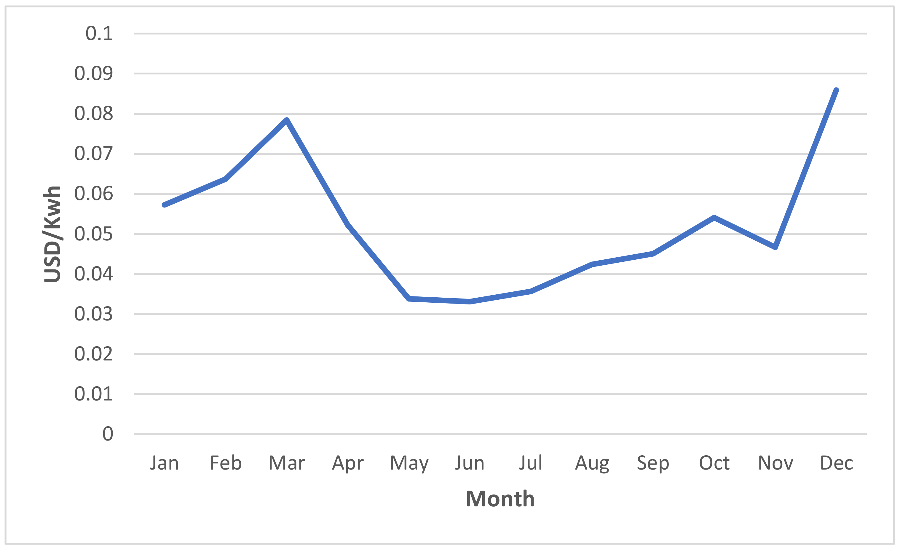
Using the cluster analysis technique, we confirmed the four hourly blocks proposed in Contreras & Rodríguez [47]: Block 1 (0–7 h), Block 2 (8–17 h), Block 3 (18–21 h), and Block 4 (22–23 h). The data were reduced from 35,064 hourly observations to 5844 four-hour observations over the four years of the period. Figure 4 shows the average monthly behavior of energy prices for 2015 to 2017.

As in the study by Contreras & Rodríguez, the highest prices are in Block 3, and the lowest price peaks are in Block 1. Price peaks occur in March and October, whereas the lowest prices occur in June and July [47].

ii.

Estimation of the price model involving climatic scenarios

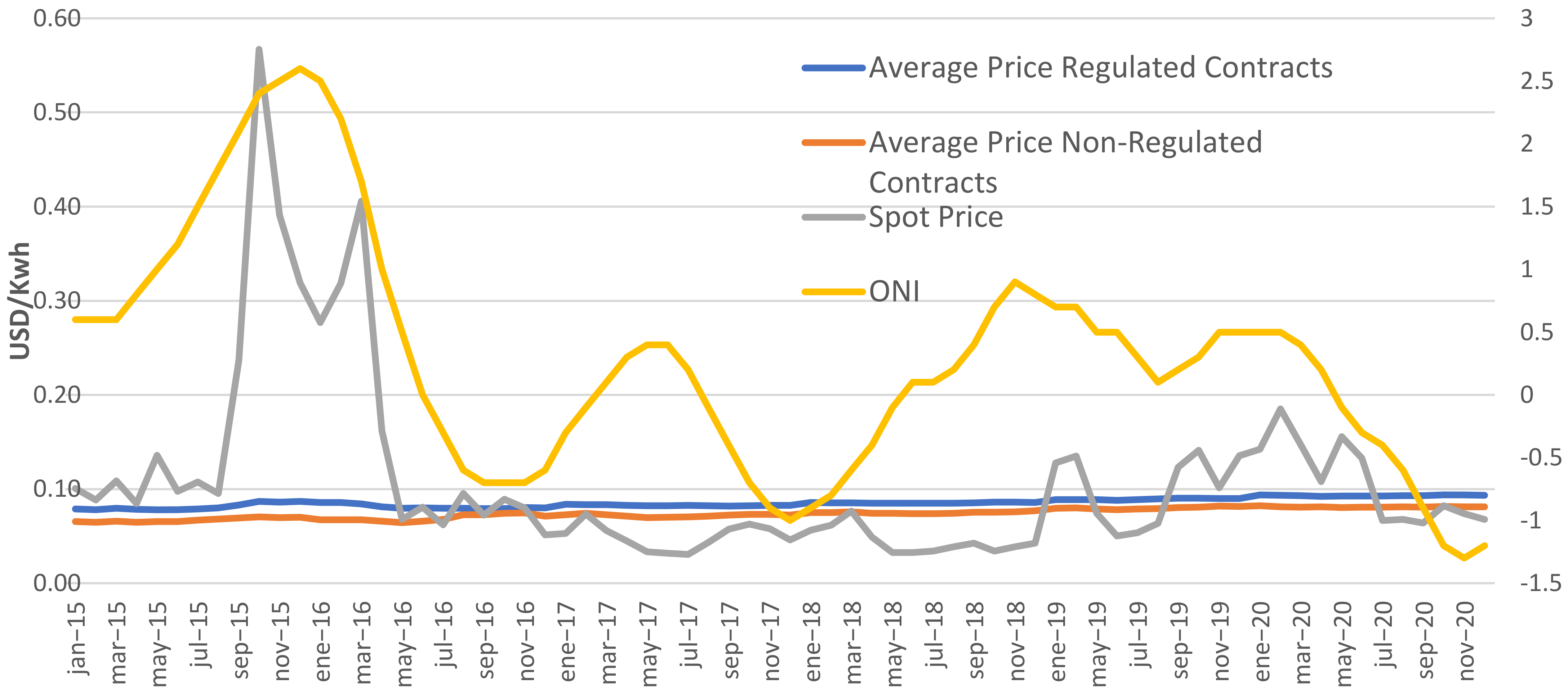
The 2015–2017 period was the basis for our price model. Since CREG has set a trigger price for capping the power exchange of USD 0.36/kWh, all prices higher than this were assumed to be USD 0.36. This period was divided into into seven climatic periods, using the ONI (see Table 2). These climatic periods were then classified into two weak El Niño periods (January-2015 to June-2015 and April-2016 to May-2016), one strong El Niño period (July-2015 to March-2016), two La Niña periods (August-2016 to December-2016 and October-2017 to December-2017) and two neutral periods (June-2016 to July-2016 and January-2017 to September-2017).

The ARIMA–GARCH method was used to model power exchange prices for each climatic period. Finally, the three models that best fit the data were selected for forecasting prices for each scenario: El Niño (April-2016 to May-2016), La Niña (October-2017 to December-2017), and a neutral period (January-2017 to Septemeber-2017).

Since the price series are not stationary, we applied a logarithmic transformation and took the difference between the logarithm of price at t and the logarithm of price at t-1. The significance of the parameters was verified at the 5% level of each of the estimated models and tests of hypotheses were performed on standardized and squared residuals. Finally, the models were used to forecast of the prices of each of the scenarios for 2018.

Table 3. GARCH model parameter estimation.

Scenario 1		Scenario 2		Scenario 3
El Niño		La Niña		Neutral Weather
ARIMA (3,1,6)		ARIMA (3,1,6)		ARIMA (3,1,6)
Parameter	Estimation	Parameter	Estimation	Parameter	Estimation
${\varphi }_1$	−0.4524	${\varphi }_1$	−0.5987	${\varphi }_1$	−0.5056
${\varphi }_2$	−1.0032	${\varphi }_2$	−0.9939	${\varphi }_2$	−0.9885
${\varphi }_3$	−0.4461	${\varphi }_3$	−0.5953	${\varphi }_3$	−0.5017
${\theta }_2$	0.6913	${\theta }_2$	0.3048	${\theta }_2$	0.4376
${\theta }_6$	0.2907	${\theta }_4$	−0.3355	${\theta }_4$	−0.2539
		${\theta }_6$	0.3272	${\theta }_6$	0.1322
GARCH (1,1)		GARCH (1,1)		GARCH (1,1)
$\omega$	0.0009	$\omega$	0.0005	$\omega$	0.0003
${\beta }_1$	0.1511	${\beta }_1$	0.2961	${\beta }_1$	0.1030
${\alpha }_1$	0.7322	${\alpha }_1$	0.6927	${\alpha }_1$	0.8779

presents the estimated parameters for the ARIMA–GARCH models chosen for each scenario.

The models for the logarithms of the block prices for each weather scenario were estimated as an ARIMA (3,1,6)–GARCH (1,1) for El Niño, La Niña, and for neutral weather. Auto regressive parameters are represented as $\varphi$ in each model. It can be seen that block prices depend on the three previous periods (the previous 24 h). Moving average parameters are represented by $\theta$ which for the La Niña scenario and the neutral weather scenario affect the previous two, four, and six hourly blocks, whereas in the El Niño scenario it only affects the second and sixth hourly blocks.

The variance model showed that using GARCH (1,1) with parameters $\omega$, $\alpha$, and $\beta$ estimated using the maximum likelihood method would be a good choice. In this case, $\omega$ is the average value at which certain variations occur, $\alpha$ is the effect of volatility that occurred in the previous period (corresponding to the ARCH term), and $\beta$ shows the prediction of the variance in the last known historical period. This means that the variance of the logarithm of block prices depends on the variance and the error of a previous period. In each of the estimated models the significance of the parameters was verified at the 5% level and tests of hypotheses on the residuals were performed.

Table 4. Goodness of fit tests for each model.

Goodness of Fit Test	El Niño	La Niña	Neutral
Mean Abs. Percent. Error (MAPE)	10.0656	8.8049	8.9412
Theil inequality coefficient	0.0691	0.0624	0.0585
Bias proportion	0.0003	0.0050	0.0026
Variance proportion	0.0000	0.0353	0.0212
Covariance proportion	0.9997	0.9596	0.9762

presents goodness of fit tests for each climatic scenario.

Five goodness of fit tests were analyzed. The mean absolute percentage error measures the accuracy of the model in terms of the percentage of error. The Theil inequality coefficient lies between 0 and 1. The smaller its value is, the better the forecast is. This test is composed of three proportions: bias, variance, and covariance whose sum is equal to 1. Bias represents a systematic error and variance indicates the ability of the forecasts to replicate the degree of variability. Both two variables are expected to be close to zero. Covariance measures the unsystematic error and is expected to be close to 1. All five tests met expectations: the mean absolute percentage error was lower than 10%, the Theil coefficient, the bias, and the variance were all very close to 0, and the covariance was greater than 0.95%. This confirms that our forecasts fluctuate in the same way as the original series.

iii.

Elaboration of the price forecast by climate scenario

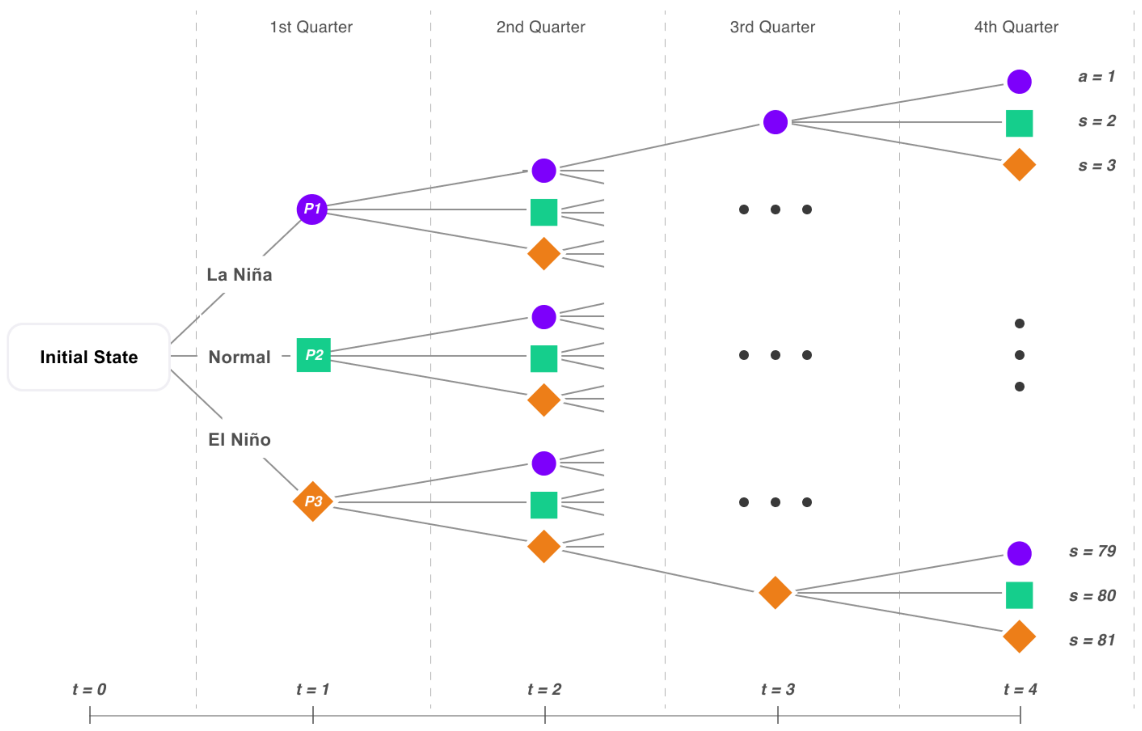
Eighty-one scenarios were constructed using the predictions of the Oceanic Niño Index of the International Institute for Climate and Society Research, and as shown in Figure 3. Each scenario has its own probability of occurrence. Of these 81 scenarios, the last 27 scenarios represent the first quarter of 2018. In that quarter, El Niño’s probability of occurrence was 0%. On this basis, 54 predicted price series were generated. Then, using the sum-product with the price series and the probability of occurrence of each scenario, we produced the forecast for prices per hourly block for 2018 (Figure 5).

iv.

Validation of price forecast

Table 5. Average monthly estimation error comparing 2018 real and forecast prices.

Month	Average Monthly Error
January	5.83%
February	4.41%
March	5.70%
April	12.18%
May	6.95%
June	4.91%
July	12.60%
August	15.47%
September	11.86%
October	14.68%
November	9.35%
December	7.32%
Average	9.31%

presents the monthly average absolute errors of the forecast prices and the real prices for 2018.

The performance of the forecast prices is reasonable because the absolute errors of the year were all less than 15% except for August, for which the error was 15.47%.

II.

Contract Pricing Model

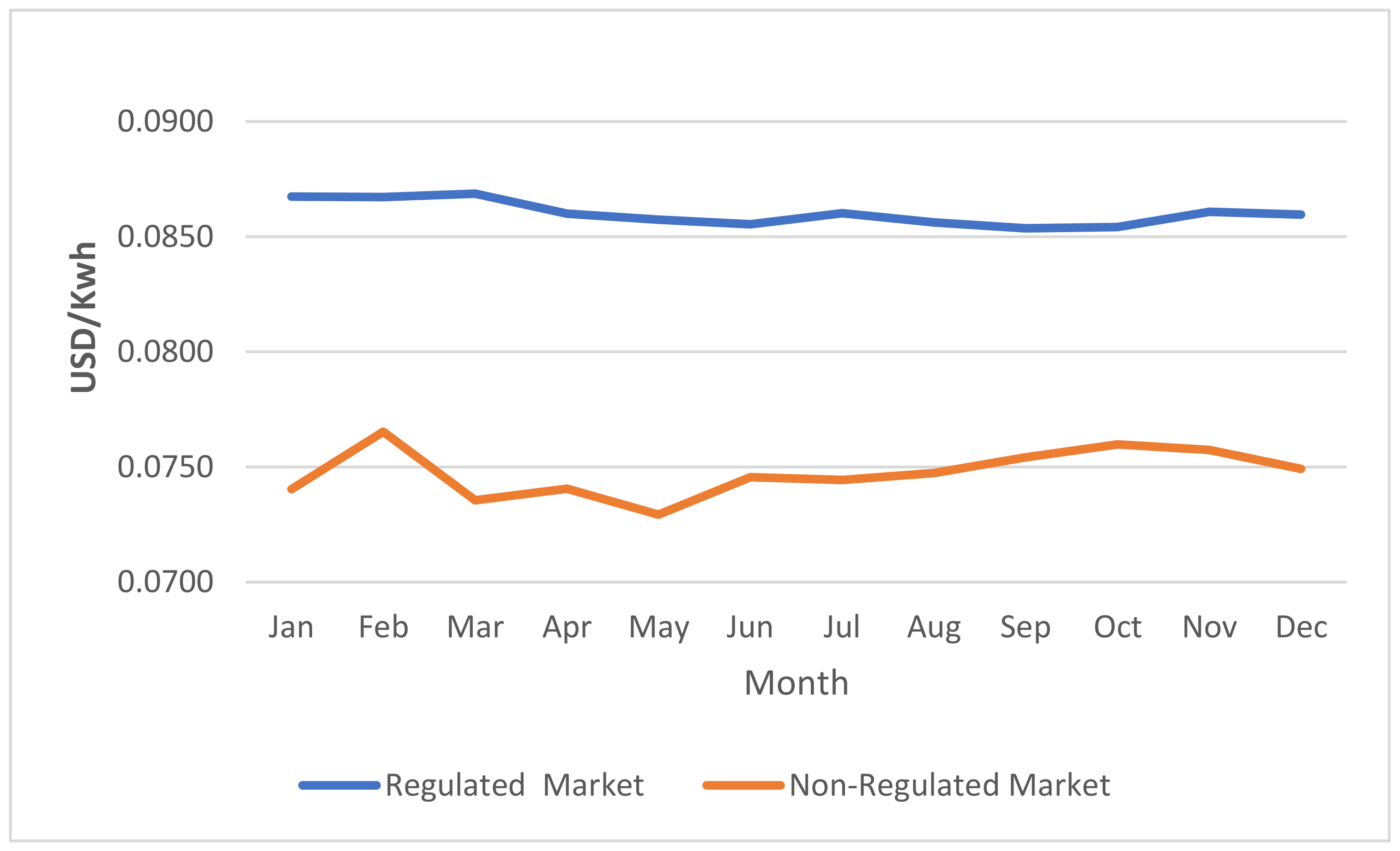
Using complete information on prices of retailers’ purchase and sale contracts from the regulated and non-regulated markets, we found that the 2017 growth rate for purchase prices in the regulated market was 7.48% and the monthly average was 0.62%. In the non-regulated market the 2017 growth rate of purchase prices was 5.53% whereas the monthly average was 0.46% (see Figure 6).

The 2015–2017 annual growth of regulated market sales prices was 6.32% whereas the monthly average was 0.52%. For the non-regulated market these figures were 2.24% and 0.20%, respectively (see Figure 7). We forecast the prices of 2018 using these estimated growth rates.

III.

Purchase Margins

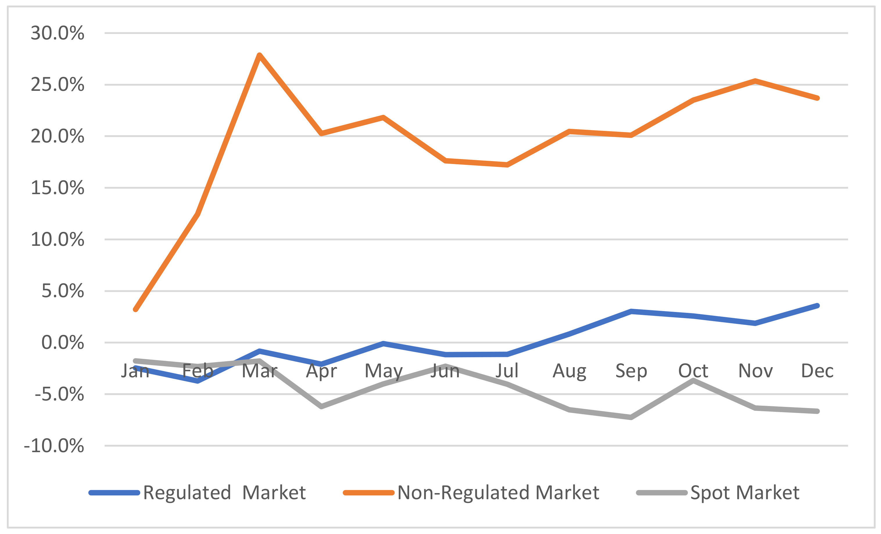
Purchase margins were calculated based on forecast prices for each strategy. Figure 8 shows estimated purchase margins of 2018 for the three purchasing strategies for retailers operating in the country: energy purchases in the power exchange, non-regulated bilateral contracts, and regulated bilateral contracts.

Volatility was greatest for spot purchases on the power exchange, and the 2018 forecast’s average purchase margin for the power exchange was −4.409% with a standard deviation of 2.090%. Profit margins were highest, on average 19.462% per month, for the non-regulated market, but volatility was also highest here, with a standard deviation of 6.527%. On the other hand, the regulated market’s monthly average margin was just 0.027% with positive margins for some months and negative margins for others. Volatility was very similar to that of the power exchange, with a standard deviation of 2.340%. In general, a retailer can hedge against the risks of spot prices with bilateral contracts, so many retailers prefer to contract in advance for longer periods.

Table 6. Descriptive statistics comparing actual and forecast margins of each strategy for 2018.

Strategy	Regulated Market		Non−Regulated Market		Power Exchange
Descriptive Statistics	Actual	Forecast	Actual	Forecast	Actual	Forecast
Average return	0.81%	0.03%	20.64%	19.46%	−6.82%	−4.41%
Standard deviation	2.32%	2.34%	2.68%	6.53%	3.90%	2.09%
Skewness	−1.48	0.11	−0.56	−1.45	−0.24	−0.02
Kurtosis	3.14	−1.13	1.08	2.83	−1.09	−1.80
Range	8.76%	7.30%	10.15%	24.65%	12.37%	5.48%
Minimum	−5.10%	−3.73%	14.83%	3.21%	−13.31%	−7.26%
Maximum	3.66%	3.58%	24.98%	27.86%	−0.93%	−1.78%
First Quarter
Average return	−1.77%	−2.34%	19.69%	14.51%	−4.24%	−1.96%
Standard deviation	2.89%	1.44%	4.60%	12.45%	1.42%	0.31%
Second Quarter
Average return	0.33%	1.48%	19.52%	2.08%	−6.50%	4.09%
Standard deviation	1.48%	0.99%	2.08%	2.12%	4.09%	1.95%
Third Quarter
Average return	1.83%	0.90%	21.49%	19.26%	−10.47%	−5.94%
Standard deviation	0.31%	2.07%	0.02%	1.76%	3.12%	1.69%
Fourth Quarter
Average return	2.85%	2.67%	21.85%	24.18%	−6.08%	−5.56%
Standard deviation	0.99%	0.86%	2.75%	1.02%	4.91%	1.65%

presents descriptive statistics for actual and forecast purchase margins.

The highest returns occur in the non-regulated market. As expected, the greatest volatility occurs in the actual purchase margins of the power exchange. Forecast purchase margin behavior is similar to that of actual margins, so these forecasts should be useful for improving retailers’ portfolio decisions.

IV.

Multi-Period Strategy

We calculated weights for each purchase strategy to compare results for actual and forecast data from 2018. We used the mean-variance portfolio and two multi-period portfolio models: “Buy and Hold” and “Fixed-Mix”.

i.

Estimation of the “Buy and Hold” portfolio

We used the mean-variance model for both predicted average purchase margins and actual average purchase margins for 2018 for allocation of portfolios in the “Buy and Hold” strategy.

Table 7. Results of the “Buy and Hold” strategy.

Portfolio	Regulated Market	Non-Regulated Market	Power Exchange	Expected Risk	Expected Purchase Margin	Actual Risk	Actual Purchase Margin
Minimum Risk	46.61%	0.00%	53.39%	0.87%	−2.34%	2.02%	−3.27%
2	37.39%	10.33%	52.28%	1.07%	−0.28%	1.97%	−1.13%
3	31.95%	16.03%	52.02%	1.27%	0.83%	1.96%	0.02%
4	27.28%	20.93%	51.79%	1.47%	1.80%	1.96%	1.01%
5	29.73%	24.00%	46.27%	1.67%	2.64%	1.83%	2.04%
Medium Risk	40.66%	24.00%	35.34%	1.87%	3.12%	1.64%	2.87%
6	49.07%	24.00%	26.93%	2.07%	3.50%	1.59%	3.51%
7	56.46%	24.00%	19.54%	2.27%	3.82%	1.64%	4.08%
8	63.29%	24.00%	12.71%	2.47%	4.13%	1.74%	4.60%
9	69.77%	24.00%	6.23%	2.67%	4.41%	1.89%	5.09%
Maximum Risk	76.00%	24.00%	0.00%	2.87%	4.69%	2.06%	5.57%

presents 11 points that correspond to an efficient portfolio on the Markowitz efficient frontier for the forecast margins. Each of the portfolios is evaluated using both margins and the matrix of variance and covariance to obtain the risk and the real margins.

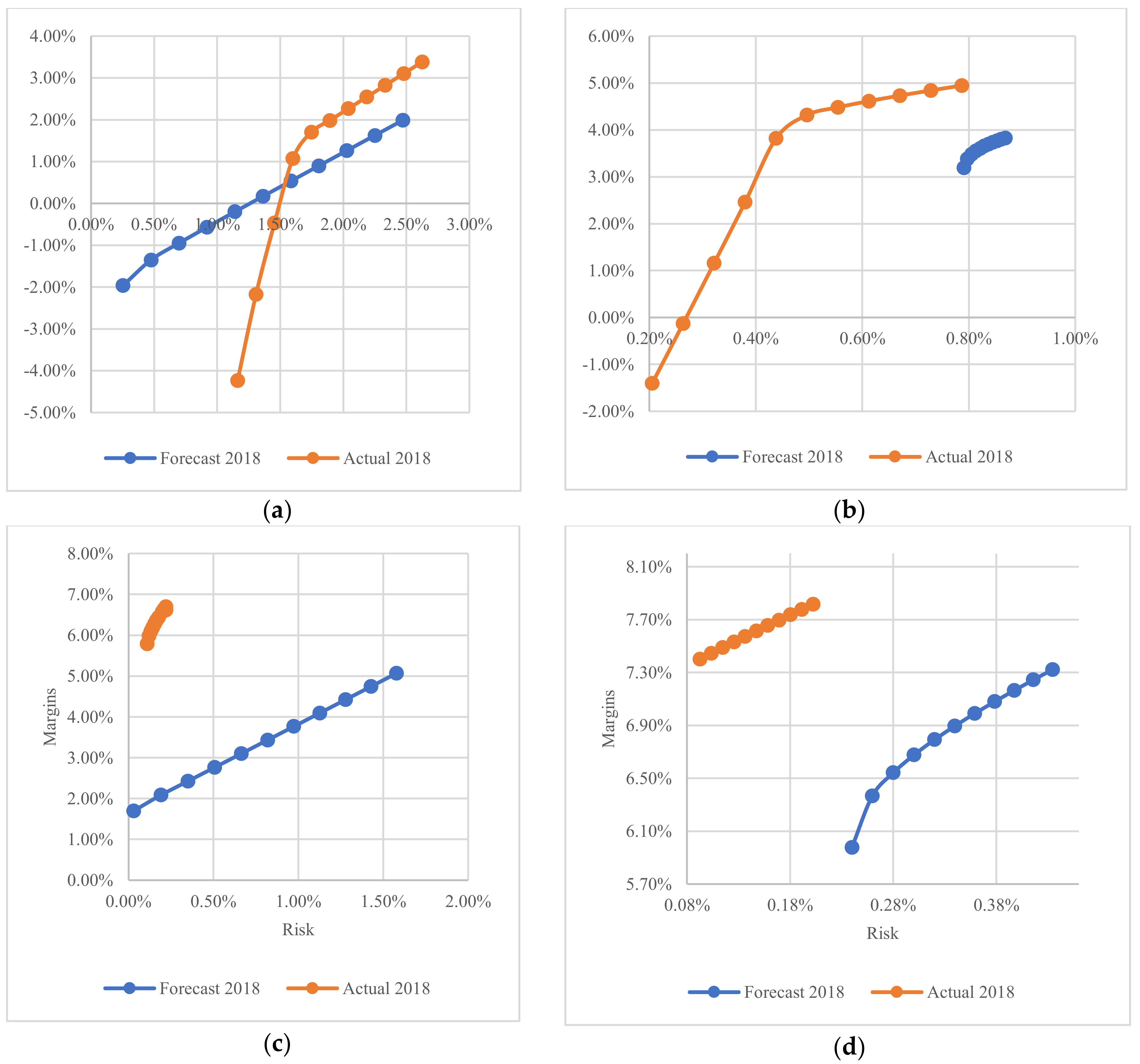
We can see that in this strategy the expected purchase margins are very close to the purchase margins that would have been caused by those decisions. Figure 9 presents efficient frontiers for the actual and forecast data from 2018. The average purchase margins and the risk for the efficient frontier of the actual data were compared with the real information for 2018. Each of the portfolios obtained with the forecast data was evaluated.

The results show that the most efficient portfolios are those that allow margins over 3% while also maintaining relatively low levels of risk. Portfolios including more than 50% of purchases on the power exchange have actual risks that are much higher than expected.

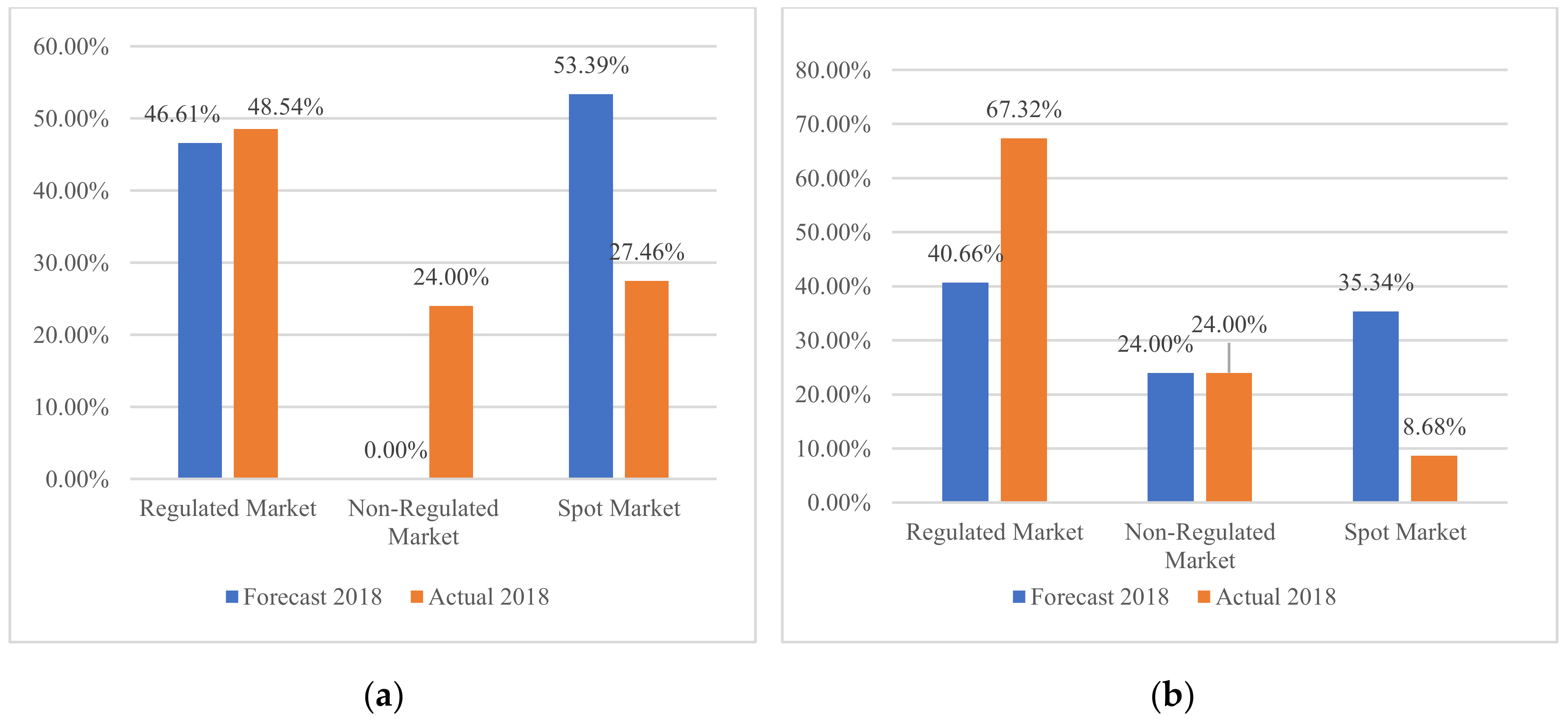
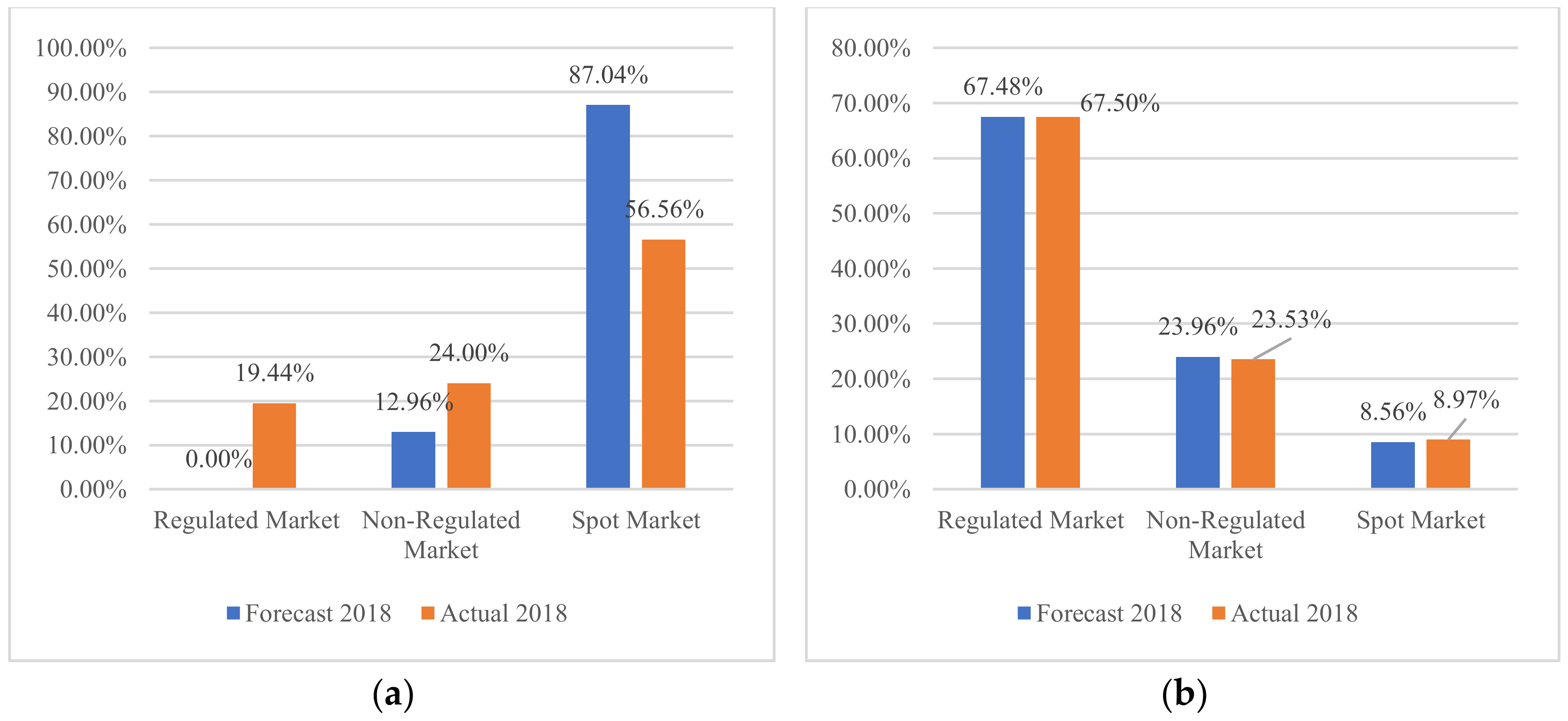
To contrast the retailers’ various possible decisions, Figure 10 presents the portfolio weights of purchases in the three markets in the minimum-, maximum-, and medium-risk portfolios. It compares the predicted data against the complete real information.

The result shows that at any point on the efficient frontier with the actual data of 2018, the portfolios will be allocated with maximum purchases of 24% in the non-regulated market. This will generate returns of 3.5% in the minimum-risk portfolio, 4.91% in the medium-risk portfolio and 5.6% in the maximum-risk portfolio. At both frontiers, the greatest risk is derived from portfolios with high proportions of purchases in the power exchange.

ii.

Estimation of the “Fixed-Mix” portfolio

The same purchase margin data was used for each “Fixed-Mix” portfolio purchase strategy as in the previous portfolios, but this model allows rebalancing every three months based on new information in an effort towards optimization.

Table 8. Descriptive statistics for 2018 power exchange purchase margins by quarter comparing forecast and actual data.

Quarter	First		Second		Third		Fourth
Statistics	Actual	Forecast	Actual	Forecast	Actual	Forecast	Actual	Forecast
Average return	−4.24%	−1.96%	−6.50%	−4.18%	−10.47%	−5.94%	−6.08%	−5.56%
Standard deviation	1.42%	0.31%	4.09%	1.95%	3.12%	1.69%	4.91%	1.65%
Skewness	−0.70	−1.73	−1.02	−0.38	0.73	1.38	0.47	1.65
Range	2.82%	0.54%	8.00%	3.90%	6.18%	3.22%	9.78%	3.00%
Minimum	−5.76%	−2.32%	−10.99%	−6.21%	−13.31%	−7.26%	−10.72%	−6.67%
Maximum	−2.94%	−1.78%	−2.99%	−2.31%	−7.12%	−4.04%	−0.93%	−3.67%

presents descriptive statistics for forecast and actual purchase margins for the power exchange for each quarter.

This strategy has much greater variation between forecast data and actual data than the purchase of energy through bilateral contracts. It seems that the forecast data is more stable than the actual data since the forecast data has lower losses and lower variance in each quarter with respect to returns. Nevertheless, there are still commonalities such as the fact that the minimum average return and the highest variance of returns in both forecast and actual data occur in the third quarter. Furthermore, the signs of bias are consistent in both data sets. Due to rebalancing of weights every period in the “Fixed-Mix” model, an efficient frontier is created in each period, as can be seen in Figure 11.

In this figure, the frontier formed by predicted data is compared with the results obtained (margin and risk) from the portfolios created with the actual data for 2018. As in the “Buy and Hold” model, portfolios that allow optimization of retailers’ purchase margins are generally those in which when the risk raises the midpoint, given that portfolios obtain much more risk than expected for lower values.

Table 9. Results of the “Fixed-Mix” strategy.

Quarters	Portfolio	Regulated Market	Non-Regulated Market	Power Exchange	Expected Risk	Expected Margin	Margin Actual Data
First	Minimum Risk	0.00%	0.00%	100.00%	0.25%	−1.96%	−4.24%
	Medium Risk	0.00%	12.96%	87.04%	1.36%	0.17%	−1.14%
	Maximum Risk	0.00%	24.00%	76.00%	2.47%	1.99%	1.50%
Second	Minimum Risk	48.14%	24.48%	27.38%	0.79%	3.19%	3.16%
	Medium Risk	67.48%	23.96%	8.56%	0.83%	3.66%	4.34%
	Maximum Risk	76.47%	23.53%	0.00%	0.87%	3.83%	4.85%
Third	Minimum Risk	24.31%	23.71%	51.98%	0.03%	1.70%	0.09%
	Medium Risk	51.83%	23.12%	25.05%	0.82%	3.43%	3.29%
	Maximum Risk	77.32%	22.68%	0.00%	1.58%	5.07%	6.29%
Fourth	Minimum Risk	55.94%	23.32%	20.74%	0.24%	5.98%	3.86%
	Medium Risk	70.52%	22.38%	7.11%	0.34%	6.90%	5.35%
	Maximum Risk	78.36%	21.64%	0.00%	0.43%	7.32%	6.09%

presents the weights and expected purchase margins and standard deviations of the three portfolios for each quarter. It shows the weights for each purchasing strategy, the risks and purchase margins for the forecast data, and the margins that a retailer could obtain by evaluating portfolios formed with the actual 2018 data.

As can be observed, higher risk corresponds to a higher percentage of purchases in the power exchange which accords with the logic that this market is more volatile. To obtain higher returns without such recourse to the power exchange, retailers need to allocate the maximum weight available to bilateral contracts in the non-regulated market. However, in the first quarter something contradictory happens, because the minimum risk portfolio places the greatest weight in the power exchange. This can be explained by the fact that this quarter’s climatic scenario has the highest probability of La Niña (see Table 1) which is reflected in the lowest volatility of the spot price in that quarter (see Table 6).

These results also confirm the observation in Figure 11 that margins obtained with the actual data are closer to the margins obtained by medium- and higher-risk portfolios. Medium-risk portfolios with more moderate attitudes allow greater diversification of strategies. As a result, the forecast portfolios perform better. Using the forecast data, a purchase margin of −1.14% would have been obtained in the first quarter, whereas with the actual data, 1.98% would have been obtained given that the loss in the power exchange would have been greater than expected. For the second quarter, the composition of the portfolios is very similar; margins of 4.34% would have been obtained with forecast data, higher than the 4.23% that would be obtained with portfolio formation based on the actual 2018 data. With complete information, the third quarter purchase margin obtained would be 5.99% whereas the fourth quarter margin would be 6.79%. With the forecast data, the final result for these quarters would have been 3.29% and 5.35%, respectively, because these portfolios give greater weight to the power-exchange-limiting margins, while allowing a more balanced portfolio.

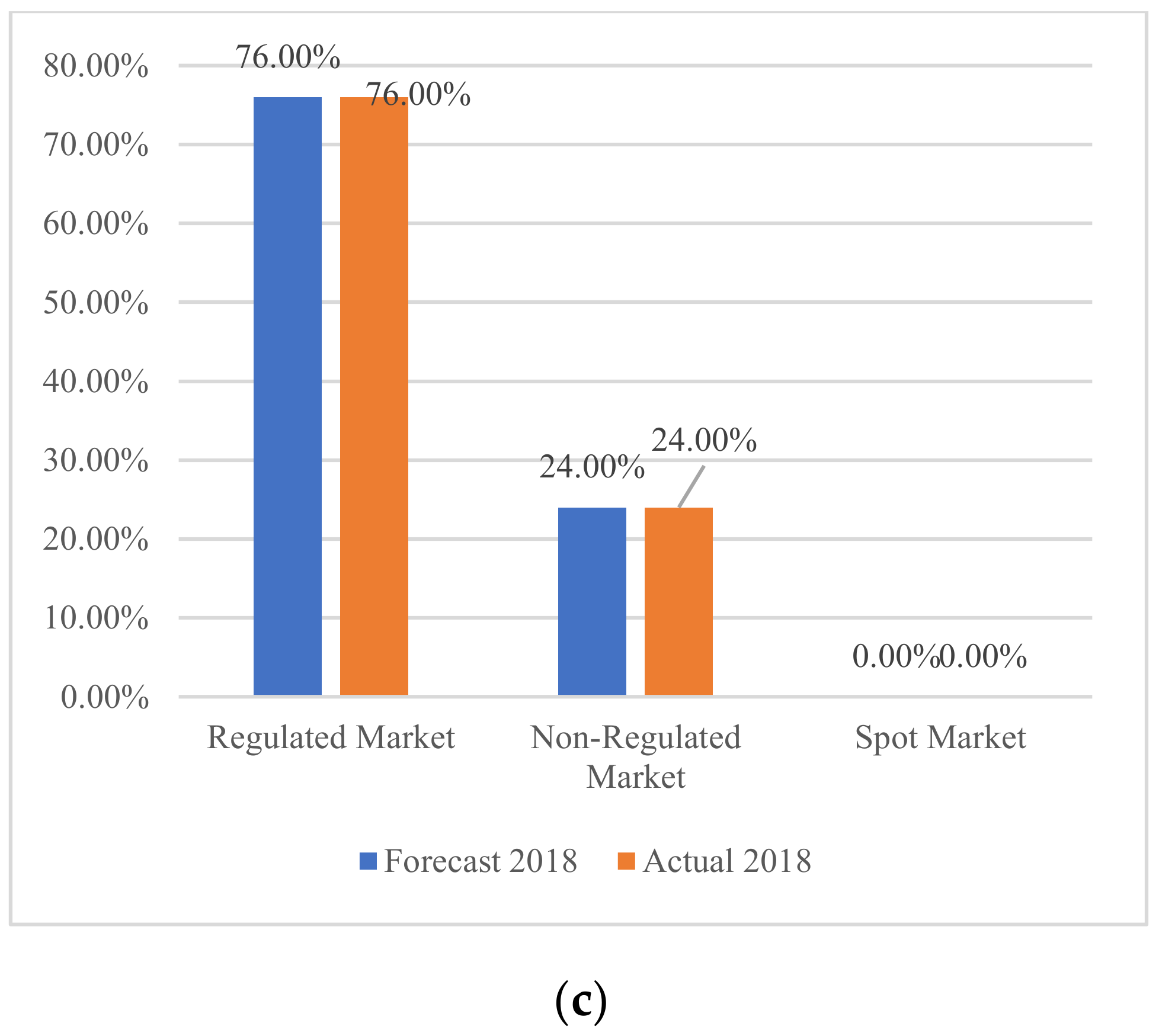
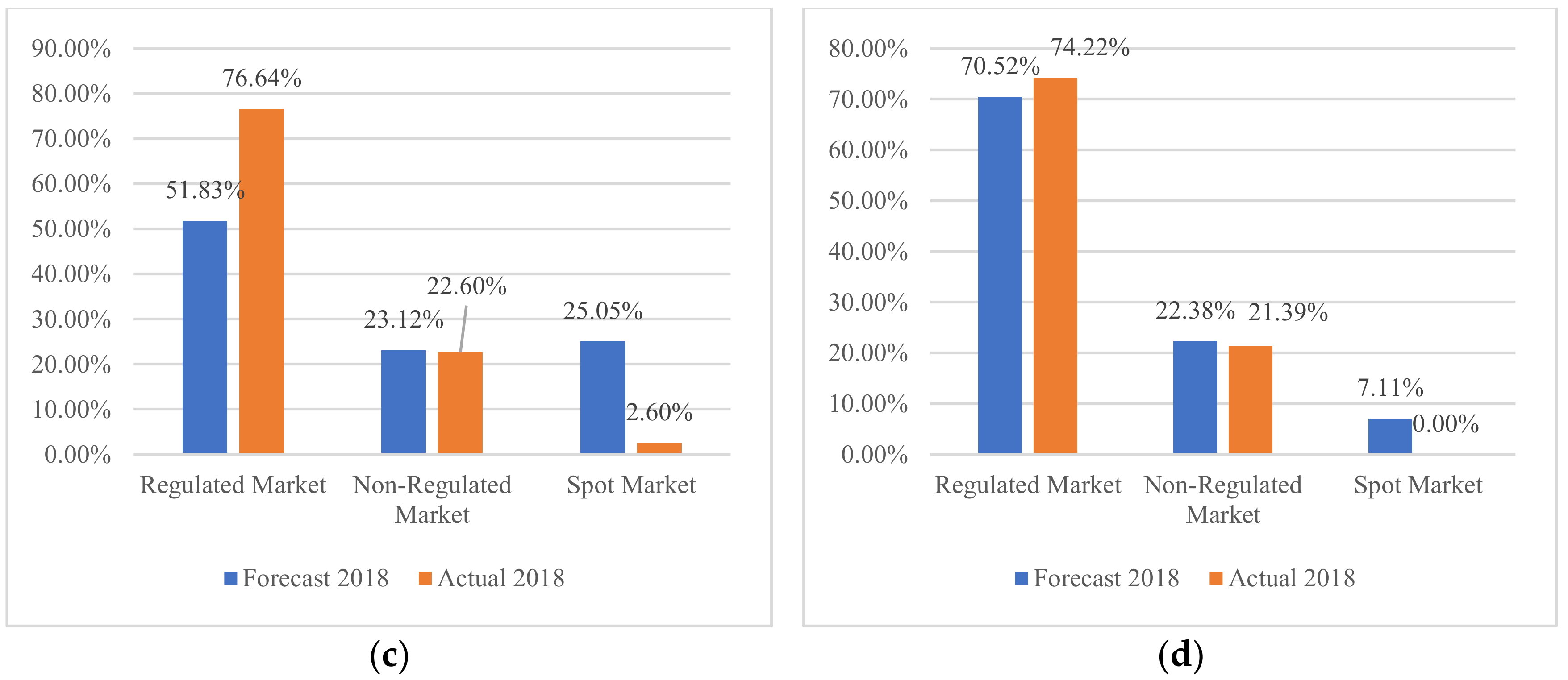
It is important to recognize that this analysis allows the use of more information between periods than the “Buy and Hold” strategy. Since the volatility of power exchange prices varies greatly between periods, this strategy can provide benefits. Figure 12 compares portfolios based on forecast data and those based on 2018 actual data.

A comparison of the weighting of portfolios created with forecast information and those created with actual information for each quarter of 2018 shows great similarities in every quarter except for the first quarter. Although in the minimum-risk portfolio we would have 100% for the power exchange with actual and forecast data, the maximum-risk portfolio based on the actual data is more like all the maximum-risk portfolios where the weights are distributed more evenly with purchases in the market for bilateral contracts and with the maximum participation possible in the non-regulated market. The results show that exceeding overall medium risk allows a portfolio to maximize margins for that portfolio’s minimum risk purchases which cannot be achieved with an overall lower portfolio risk.

V.

Portfolio Performance Evaluation

The performance of each portfolio was evaluated using the backtesting method. First, we evaluated the results obtained with the actual data for 2018 for all three portfolios in both of the two strategies.

Table 10. Results of the “Buy and Hold” and “Fixed-Mix” strategy.

	“Buy and Hold”			“Fixed-Mix”
Month	Minimum Risk	Medium Risk	Maximum Risk	Minimum Risk	Medium Risk	Maximum Risk
January	−5.451%	−0.550%	−0.315%	−5.760%	−3.093%	−0.819%
February	−2.281%	4.213%	5.523%	−4.010%	−0.385%	2.705%
March	−1.525%	3.864%	4.938%	−2.941%	0.065%	2.629%
April	−4.921%	1.318%	5.920%	2.432%	4.799%	5.844%
May	−3.140%	2.298%	4.101%	2.795%	3.657%	4.013%
June	−1.889%	3.949%	4.785%	4.246%	4.573%	4.680%
July	−3.111%	3.239%	6.281%	1.748%	3.948%	6.018%
August	−6.213%	1.230%	6.607%	−1.360%	2.622%	6.349%
September	−4.893%	2.131%	6.757%	−0.105%	3.306%	6.500%
October	−4.909%	2.916%	7.318%	4.576%	6.055%	6.770%
November	−2.057%	3.927%	7.366%	5.228%	6.388%	6.951%
December	1.209%	5.915%	7.538%	6.475%	6.949%	7.157%
Average return	−3.26%	2.87%	5.57%	1.11%	3.24%	4.90%

shows the purchase margins that would have been obtained in each month of 2018.

Results for the “Fixed-Mix” strategy are better even for the minimum-risk portfolio that also has the smallest margin. It is certain that a strategy that allows making changes over time can better take into account volatility in the power exchange and margins that vary from one period to another in a way that can generate losses if not taken into account. Considering price changes due to changing weather patterns can clearly improve risk-management decision-making.

VI.

Portfolio evaluation through backtesting

Table 11. Results of backtesting criteria.

	“Buy and Hold”			“Fixed-Mix”
Indicator	Minimum Risk	Medium Risk	Maximum Risk	Minimum Risk	Medium Risk	Maximum Risk
Max drawdown	0.047	0.029	0.018	0.056	0.022	0.018
Sharpe ratio	−6.436	6.830	12.272	1.040	4.459	9.344
Sterling ratio	−0.642	0.956	3.793	0.153	1.581	3.187
Omega ratio	0.030	63.691	213.078	1.940	12.180	72.766

presents the four criteria that were used to evaluate how a portfolio would have performed to help retailers make the best decisions.

Analyses of the different criteria show that for portfolios with minimum risk, the “Fixed-Mix” strategy outperforms “Buy and Hold” in all the three portfolio evaluation ratios which indicates that these portfolios receive greater returns relative to the expected level of risk. Although this strategy also has a higher maximum drawdown for the minimum-risk portfolio than the “Buy and Hold” strategy for the same portfolio, the “Fixed-Mix” strategy is still preferred.

The Sharpe and Omega ratios indicate that the “Buy and Hold” strategy is better for the medium-risk portfolio given that it has a higher return for each unit of risk and that the probability of positive margins is much higher than the probability of negative months, but the maximum drawdown and the Sterling ratio indicate that the “Fixed-Mix” strategy is best. For our case it is also important to note that the annual volatility in the “Buy and Hold” strategy is not quite half the volatility in the “Fixed-Mix” portfolio without any penalty in the annual margins. Although the “Buy and Hold” portfolio had a maximum drawdown of 0.029, this number is quite close to the 0.022 of the “Fixed-Mix” portfolio. Even though both have similar annual margins, the “Buy and Hold” strategy is advisable if a moderate risk is expected since its volatility is far less than that of the “Fixed-Mix” portfolio, and the probability of positive margins is much higher than for any other strategy.

Finally, we can ensure that the maximum-risk portfolio’s performance improves using a “Fixed-Mix” strategy with respect to the risk taken by using the “Buy and Hold” strategy since it allows a greater margin at lower annual volatility. This is true even though the maximum drawdowns of the two strategies are the same size as the three high-performing ratios for the “Buy and Hold” portfolio, indicating that the portfolio will receive greater returns per unit of risk.

5. Conclusions

This study proposes an optimal composition for energy retailers’ energy purchase portfolios. Our application was developed with real and forecast information for 2018 in the Colombian electricity market. The portfolio theory proposed by Markowitz [11,12] was extended to consider a planning analysis for one year, for which two multi-period acquisition strategies were proposed: a simple portfolio extension using the “Buy and Hold” strategy for a single period, and the “Fixed-Mix” strategy that allows rebalancing of the information for each period. In the latter case, the one-year period was divided into four quarters since the NOAA’s climate reports are quarterly.

In the literature, some authors have developed several methods for forecasting Colombian electricity prices. We propose a forecasting model for prices that involves various possible climatic scenarios, each with its own associated probability. This type of model best adjusts for the behavior of real prices. The multi-period approach was proposed to enable retailers to maximize their purchase margins by using better planning strategies. With this approach, retailers can choose short-term purchase strategies that are in accordance with the needs of the market and that react to unexpected price variations due to climatic changes.

The results show that portfolio rebalancing in each quarter only produces better performances in portfolios constructed to minimize risk. Nevertheless, portfolios in which the three purchasing strategies including the power exchange were used, annual volatility ended up being higher than for portfolios that had higher risks. Given that the very great volatility of the power exchange, the strategy of rebalancing portfolios every quarter provvides better protection against power exchange price volatility. Taken altogether, these factors clearly show that the “Fixed-Mix” portfolio strategy is the most likely to obtain optimal results.

In contrast, for portfolios that have higher expected margins, the best multi-period strategy to follow is “Buy and Hold”. Although in principle a strategy that allows rebalancing portfolio weights might be better, our forecast of the prices for each strategy includes price volatility due to weather and is a remarkably good fit to the actual data. It shows that the “Buy and Hold” strategy is the strongest in these cases. In addition, the “Buy and Hold” strategy was the least volatile for moderate-risk portfolios which could indicate that retailers should be neither extremely conservative nor take extreme risks. Rather, it suggests they should follow a middle course by balancing purchases in bilateral contract markets and in the power exchange. This strategy is the most likely to control retailers’ risks while providing good margins.

References

1. McNeil, A.J.; Frey, R.; Embrechts, P. Quantitative Risk Management: Concepts, Techniques and Tools—Revised Edition; Princeton University Press: Princeton, NJ, USA, 2005. [Google Scholar]
2. Kempers, M.; Leitterstorf, M.P.; Kammerlander, N. Risk Behavior of Family Firms: A Literature Review, Framework, and Research Agenda. In The Palgrave Handbook of Heterogeneity among Family Firms; Palgrave Macmillan: London, UK, 2019; pp. 431–460. ISBN 978-3319776750. [Google Scholar] [CrossRef]
3. Mcconaughy, D.L.; Matthews, C.H.; Fialko, A.S. Founding Family Controlled Firms: Performance, Risk, and Value. J. Small Bus. Manag. 2001, 39, 31–49. [Google Scholar] [CrossRef]
4. Ruefli, T.W.; Collins, J.M.; Lacugna, J.R. Risk Measures in Strategic Management Research: Auld Lang Syne? on JSTOR. Strateg. Manag. J. 1999, 20, 167–194. [Google Scholar] [CrossRef]
5. Escribano Francés, G.; Marín-Quemada, J.M.; San Martín González, E.; Escribano Francés, G.; Marín-Quemada, J.M.; San Martín González, E. RES and risk: Renewable energy’s contribution to energy security. A portfolio-based approach. Renew. Sustain. Energy Rev. 2013, 26, 549–559. [Google Scholar] [CrossRef]
6. Higgins, R.C.; Schall, L.D. Corporate Bankruptcy and Conglomerate Merger. J. Financ. 1975, 30, 93. [Google Scholar] [CrossRef]
7. March, J.G.; Shapira, Z. Managerial Perspectives on Risk and Risk Taking. Manag. Sci. 1987, 33, 1404–1418. [Google Scholar] [CrossRef] [Green Version]
8. Goetzmann, W.N.; Kumar, A. Equity Portfolio Diversification. Rev. Financ. 2008, 12, 433–463. [Google Scholar] [CrossRef] [Green Version]
9. Hatami, A.; Seifi, H.; Sheikh-El-Eslami, M.K. A stochastic-based decision-making framework for an electricity retailer: Time-of-use pricing and electricity portfolio optimization. IEEE Trans. Power Syst. 2011, 26, 1808–1816. [Google Scholar] [CrossRef]
10. Glensk, B.; Madlener, R. Multi-period portfolio optimization of power generation assets. Oper. Res. Decis. 2013, 23, 21–38. [Google Scholar] [CrossRef]
11. Markowitz, H. Portfolio Selection. J. Financ. 1952, 7, 77–91. [Google Scholar] [CrossRef]
12. Markowitz, H. Portfolio Selection: Efficient Diversification of Investments; Yale University Press: New Haven, CT, USA, 1959; ISBN 9780300191677. [Google Scholar]
13. Charwand, M.; Ahmadi, A.; Siano, P.; Dargahi, V.; Sarno, D. Exploring the trade-off between competing objectives for electricity energy retailers through a novel multi-objective framework. Energy Convers. Manag. 2015, 91, 12–18. [Google Scholar] [CrossRef]
14. Boroumand, R.H.; Goutte, S.; Porcher, S.; Porcher, T. Hedging strategies in energy markets: The case of electricity retailers. Energy Econ. 2015, 51, 503–509. [Google Scholar] [CrossRef]
15. Algarvio, H.; Lopes, F.; Sousa, J.; Lagarto, J. Multi-agent electricity markets: Retailer portfolio optimization using Markowitz theory. Electr. Power Syst. Res. 2017, 148, 282–294. [Google Scholar] [CrossRef]
16. Contreras, J.; Rodríguez, Y.E.; Sosa, A. Construction of an efficient portfolio of power purchase decisions based on risk-diversification tradeoff. Energy Econ. 2017, 64, 286–297. [Google Scholar] [CrossRef]
17. Charwand, M.; Gitizadeh, M.; Siano, P. A new active portfolio risk management for an electricity retailer based on a drawdown risk preference. Energy 2017, 118, 387–398. [Google Scholar] [CrossRef]
18. Rocha, P.; Kuhn, D. Multistage stochastic portfolio optimisation in deregulated electricity markets using linear decision rules. Eur. J. Oper. Res. 2012, 216, 397–408. [Google Scholar] [CrossRef] [Green Version]
19. Hou, J.; Zhang, Z.; Lin, Z.; Yang, L.; Liu, X.; Jiang, Y.; He, C.; Li, J.; Wang, K.; Zhang, W.; et al. An Energy Imbalance Settlement Mechanism Considering Decision-Making Strategy of Retailers under Renewable Portfolio Standard. IEEE Access 2019, 7, 118146–118161. [Google Scholar] [CrossRef]
20. Carrión, M.; Arroyo, J.M.; Conejo, A.J. A bilevel stochastic programming approach for retailer futures market trading. IEEE Trans. Power Syst. 2009, 24, 1446–1456. [Google Scholar] [CrossRef]
21. Golmohamadi, H.; Keypour, R.; Hassanpour, A.; Davoudi, M. Optimization of green energy portfolio in retail market using stochastic programming. In Proceedings of the 2015 North American Power Symposium (NAPS), Charlotte, NC, USA, 4–6 October 2015; pp. 1–6. [Google Scholar]
22. Nojavan, S.; Mehdinejad, M.; Zare, K.; Mohammadi-Ivatloo, B. Energy procurement management for electricity retailer using new hybrid approach based on combined BICA-BPSO. Int. J. Electr. Power Energy Syst. 2015, 73, 411–419. [Google Scholar] [CrossRef]
23. Collomb, A. Dynamic Asset Allocation by Stochastic Programming Methods; Stanford University: Stanford, CA, USA, 2004. [Google Scholar]
24. Henao, F.; Rodriguez, Y.; Viteri, J.P.; Dyner, I. Optimising the insertion of renewables in the Colombian power sector. Renew. Energy 2019, 132, 81–92. [Google Scholar] [CrossRef]
25. UPME: Mining-Energy Planning Unit Proyección Demanda Energía Eléctrica y Gas Natural 2021–2035. Available online: https://www1.upme.gov.co/DemandayEficiencia/Documents/UPME_Proyeccion_Demanda_Energia_Junio_2021.pdf (accessed on 9 December 2021).
26. Dyner, I.; Larsen, E.; Franco, C.J. Games for electricity traders: Understanding risk in a deregulated industry. Energy Policy 2009, 37, 465–471. [Google Scholar] [CrossRef]
27. CREG: Commission for the Regulation of Energy and Gas Resolution 131 de 1998. Available online: http://apolo.creg.gov.co/Publicac.nsf/1aed427ff782911965256751001e9e55/c2d01cc1ae3da04a0525785a007a5fa5/$FILE/Cr131-98.pdf (accessed on 6 March 2020).
28. James, T. Energy Markets: Price Risk Management and Trading; Wiley: New York, NY, USA, 2012; ISBN 9781118580479. [Google Scholar]
29. Kettunen, J.; Salo, A.; Bunn, D.W. Optimization of Electricity Retailer’s Contract Portfolio Subject to Risk Preferences. IEEE Trans. Power Syst. 2010, 25, 117–128. [Google Scholar] [CrossRef]
30. Kharrati, S.; Kazemi, M.; Ehsan, M. Equilibria in the competitive retail electricity market considering uncertainty and risk management. Energy 2016, 106, 315–328. [Google Scholar] [CrossRef]
31. Milhomem, D.A.; Dantas, M.J.P. Analysis of new approaches used in portfolio optimization: A systematic literature review. Production 2020, 30, 1–16. [Google Scholar] [CrossRef]
32. Chapados, N. Multiperiod Problems. In Portfolio Choice Problems: An Introductory Survey of Single and Multiperiod Models; Springer: Berlin/Heidelberg, Germany, 2011; p. 96. ISBN 9781461405771. [Google Scholar]
33. Tofighian, A.A.; Moezzi, H.; Khakzar Barfuei, M.; Shafiee, M. Multi-period project portfolio selection under risk considerations and stochastic income. J. Ind. Eng. Int. 2018, 14, 571–584. [Google Scholar] [CrossRef] [Green Version]
34. Liu, Y.J.; Zhang, W.G. A multi-period fuzzy portfolio optimization model with minimum transaction lots. Eur. J. Oper. Res. 2015, 242, 933–941. [Google Scholar] [CrossRef]
35. Zhang, P.; Zhang, W.-G. Multiperiod mean absolute deviation fuzzy portfolio selection model with risk control and cardinality constraints. Fuzzy Sets Syst. 2014, 255, 74–91. [Google Scholar] [CrossRef]
36. Li, D.; Ng, W.-L. Optimal Dynamic Portfolio Selection: Multiperiod Mean-Variance Formulation. Math. Financ. 2000, 10, 387–406. [Google Scholar] [CrossRef]
37. Hui, E.; Yam, P.; Wright, J.; Chan, K. Shall we buy and hold? Evidence from Asian real estate markets. J. Prop. Invest. Finance 2014, 32, 168–186. [Google Scholar] [CrossRef]
38. Fleten, S.-E.; Wallace, S.W.; Ziemba, W.T. Hedging Electricity Portfolios via Stochastic Programming; Springer: New York, NY, USA, 2002; pp. 71–93. [Google Scholar]
39. Dempster, M.A.H.; Evstigneev, I.V.; Schenk-Hoppé, K.R. Exponential growth of fixed-mix strategies in stationary asset markets. Finance Stoch. 2003, 7, 263–276. [Google Scholar] [CrossRef]
40. Nazari, M.; Akbari Foroud, A. Optimal strategy planning for a retailer considering medium and short-term decisions. Int. J. Electr. Power Energy Syst. 2013, 45, 107–116. [Google Scholar] [CrossRef]
41. Safdarian, A.; Fotuhi-Firuzabad, M.; Lehtonen, M. A distributed algorithm for managing residential demand response in smart grids. IEEE Trans. Ind. Inform. 2014, 10, 2385–2393. [Google Scholar] [CrossRef]
42. Garcia, R.C.; Contreras, J.; VanAkkeren, M.; Garcia, J.B.C. A GARCH Forecasting Model to Predict Day-Ahead Electricity Prices. IEEE Trans. Power Syst. 2005, 20, 867–874. [Google Scholar] [CrossRef]
43. Haldrup, N.; Nielsen, M.Ø. A regime switching long memory model for electricity prices. J. Econom. 2006, 135, 349–376. [Google Scholar] [CrossRef]
44. Becker, R.; Hurn, S.; Pavlov, V. Modelling Spikes in Electricity Prices*. Econ. Rec. 2007, 83, 371–382. [Google Scholar] [CrossRef]
45. Weron, R. Heavy-tails and regime-switching in electricity prices. Math. Methods Oper. Res. 2009, 69, 457–473. [Google Scholar] [CrossRef] [Green Version]
46. Weber, M.; Prokopczuk, M. American Option Valuation: Implied Calibration of GARCH Pricing-Models. J. Futures Mark. 2011, 31, 971–994. [Google Scholar] [CrossRef]
47. Contreras, J.; Rodríguez, Y.E. GARCH-based put option valuation to maximize benefit of wind investors. Appl. Energy 2014, 136, 259–268. [Google Scholar] [CrossRef]
48. Catalão, J.P.S.; Mariano, S.J.P.S.; Mendes, V.M.F.; Ferreira, L.A.F.M. Short-term electricity prices forecasting in a competitive market: A neural network approach. Electr. Power Syst. Res. 2007, 77, 1297–1304. [Google Scholar] [CrossRef] [Green Version]
49. Geman, H.; Roncoroni, A. Understanding the fine structure of electricity prices. J. Bus. 2006, 79, 1225–1261. [Google Scholar] [CrossRef] [Green Version]
50. Bollerslev, T. Generalized autoregressive conditional heteroskedasticity. J. Econom. 1986, 31, 307–327. [Google Scholar] [CrossRef] [Green Version]
51. Engle, R.F. Autoregressive Conditional Heteroscedasticity with Estimates of the Variance of United Kingdom Inflation. Econometrica 1982, 50, 987. [Google Scholar] [CrossRef]
52. IRI: International Research Institute for Climate and Society IRI ENSO Forecast. Available online: https://iri.columbia.edu/our-expertise/climate/forecasts/enso/2017-December-quick-look/?enso_tab=enso-sst_table (accessed on 9 December 2021).
53. U.S. Department of Commerce National Oceanic and Atmospheric Administration. Available online: https://www.noaa.gov/ (accessed on 20 August 2019).
54. Chekhlov, A.; Uryasev, S.; Zabarankin, M. Drawdown measure in portfolio optimization. Int. J. Theor. Appl. Finance 2011, 8, 13–58. [Google Scholar] [CrossRef]
55. Sharpe, W. Mutual Fund Performance. J. Bus. 1966, 39, 119–138. [Google Scholar] [CrossRef]
56. Bacon, C.R. Practical Portfolio Performance Measurement and Attribution; John Wiley & Sons: Hoboken, NJ, USA, 2008; Volume 546. [Google Scholar]
57. Keating, C.; Shadwick, W. A universal performance measure. J. Perform. Meas. 2002, 6, 59–84. [Google Scholar]
Figure 1. Evolution of contract prices of regulated and non-regulated markets, and power exchange (USD/kWh). Source: XM S.A. E.S.P.
Energies 15 03012 g001
Figure 2. Steps for multiperiod power purchasing portfolios.
Energies 15 03012 g002
Figure 3. Climatic scenario probability tree.
Energies 15 03012 g003
Figure 4. Average behavior of monthly electricity prices in Colombia in 2015–2017.
Energies 15 03012 g004
Figure 5. Forecast averages of power exchange prices for 2018.
Energies 15 03012 g005
Figure 6. Average monthly behavior of forecast purchase prices for 2018.
Energies 15 03012 g006
Figure 7. Average monthly behavior of forecast sale prices for 2018.
Energies 15 03012 g007
Figure 8. Purchase margins forecast for each strategy for 2018.
Energies 15 03012 g008
Figure 9. Comparison of efficient frontier created based on “Buy and Hold” portfolio.
Energies 15 03012 g009
Figure 10. Minimum risk, medium risk and maximum purchase margin portfolio weights based on “Buy and Hold” strategies compared with actual data. (a) Minimum Risk Portfolio. (b) Medium Risk Portfolio. (c) Maximum Risk Portfolio.
Energies 15 03012 g010aEnergies 15 03012 g010b
Figure 11. Comparison of efficient frontier created based on “Buy and Hold” portfolio. (a) 1st Quarter 2018. (b) 2nd Quarter 2018. (c) 3rd Quarter 2018. (d) 4th Quarter 2018.
Energies 15 03012 g011
Figure 12. Medium-risk portfolios in each quarter, comparison of forecast with actual data for 2018. (a) 1st Quarter. (b) 2nd Quarter. (c) 3rd Quarter. (d) 4th Quarter.
Energies 15 03012 g012aEnergies 15 03012 g012b