Table A1.
Correlation coefficients of predicted and actual cloud modification factor (CMF) time series for 4 lead time steps (+1 to +4) in 2020 for Athens.
| Method | +1 | +2 | +3 | +4 |
|---|
| pers | 0.9157 | 0.8323 | 0.7867 | 0.7509 |
| mc_a | 0.9164 | 0.8394 | 0.7929 | 0.7587 |
| mc_b | 0.9164 | 0.816 | 0.7498 | 0.6981 |
| neib | 0.8332 | 0.7626 | 0.7329 | 0.7065 |
| hyb_m | 0.9174 | 0.8475 | 0.8069 | 0.7821 |
| hyb_r | 0.9176 | 0.8406 | 0.7807 | 0.7574 |
Table A2.
Correlation coefficients of predicted and actual CMF time series for 4 lead time steps (+1 to +4) in 2020 for Bucharest.
| Method | +1 | +2 | +3 | +4 |
|---|
| pers | 0.9226 | 0.8457 | 0.8023 | 0.7663 |
| mc_a | 0.955 | 0.8811 | 0.8281 | 0.7854 |
| mc_b | 0.955 | 0.885 | 0.8136 | 0.7549 |
| neib | 0.8953 | 0.8281 | 0.7943 | 0.7631 |
| hyb_m | 0.9547 | 0.8919 | 0.8381 | 0.7954 |
| hyb_r | 0.9547 | 0.8892 | 0.8365 | 0.7962 |
Table A3.
Correlation coefficients of predicted and actual CMF time series for 4 lead time steps (+1 to +4) in 2020 for Helsinki.
| Method | +1 | +2 | +3 | +4 |
|---|
| pers | 0.8974 | 0.7858 | 0.7319 | 0.6943 |
| mc_a | 0.9424 | 0.8408 | 0.7715 | 0.7189 |
| mc_b | 0.9424 | 0.8413 | 0.7488 | 0.6651 |
| neib | 0.8878 | 0.7831 | 0.7342 | 0.6982 |
| hyb_m | 0.941 | 0.8551 | 0.8094 | 0.7725 |
| hyb_r | 0.9418 | 0.8536 | 0.81 | 0.7696 |
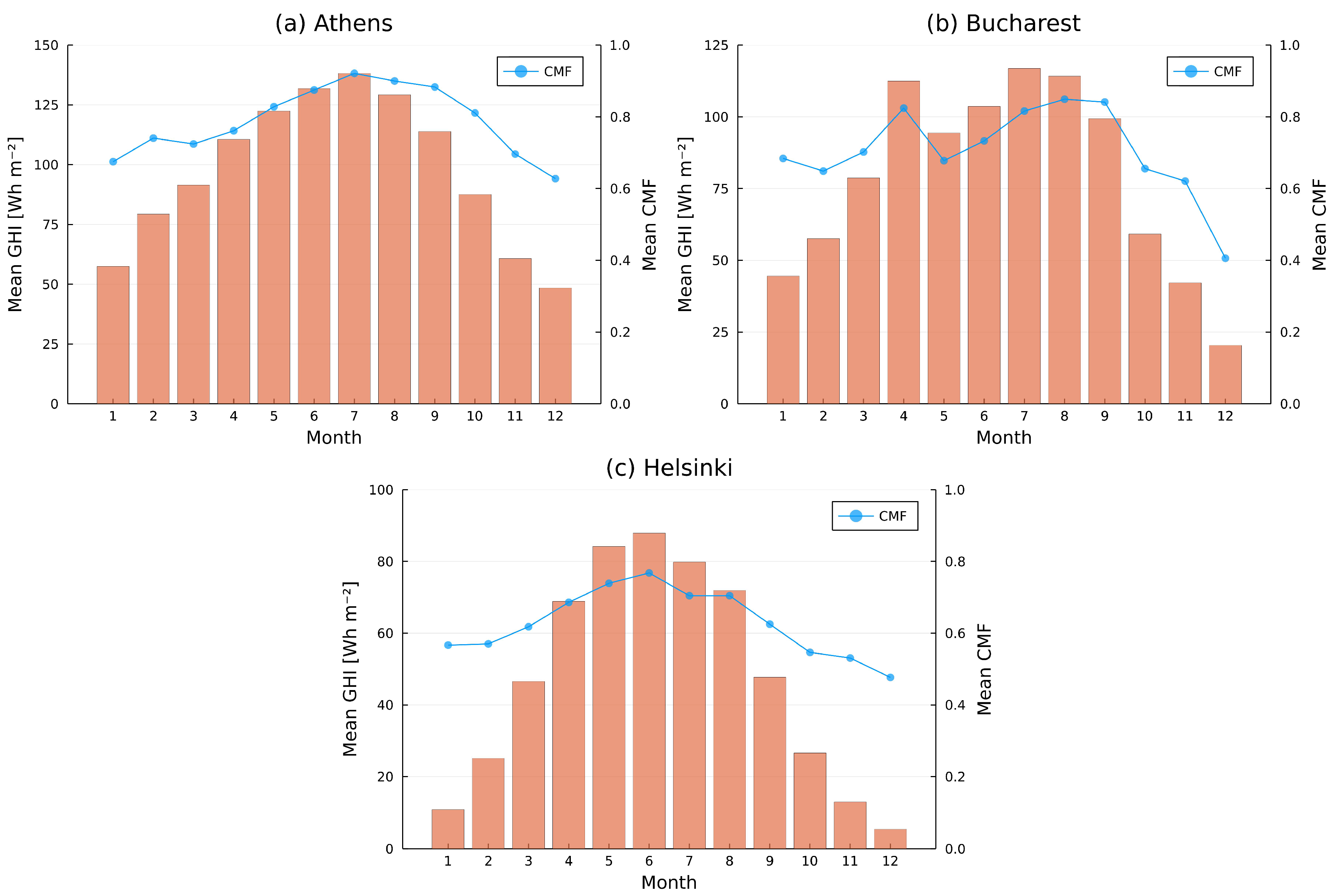
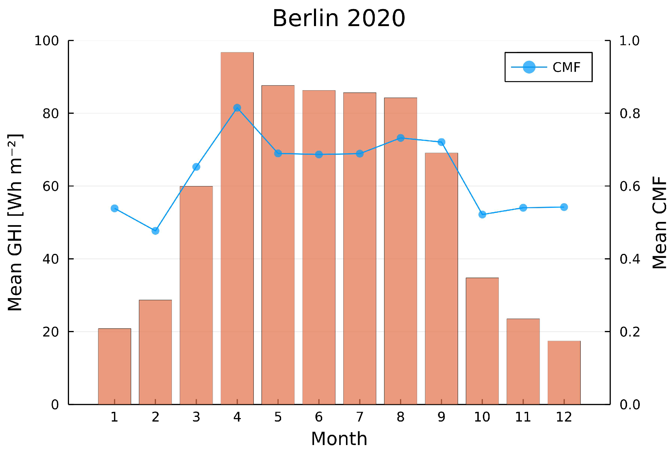
Figure A1.
Daily mean global horizontal irradiation (GHI) for each month (orange bars, left axis) and monthly mean cloud modification factor (CMF; blue curves, right axis) in 2020 for (a) Athens, (b) Bucharest, and (c) Helsinki.
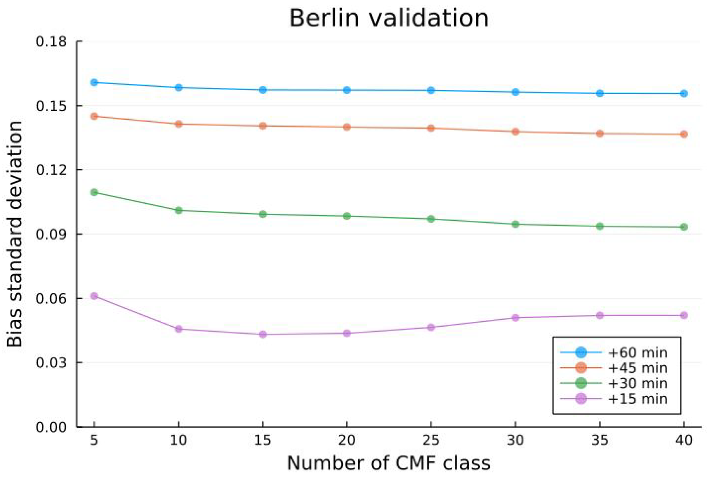
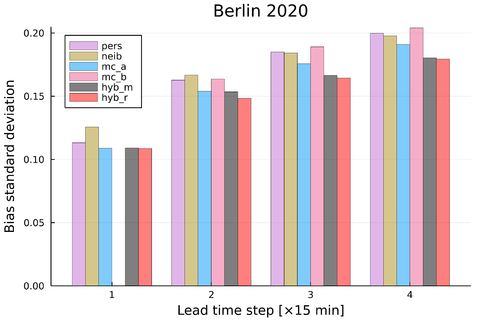
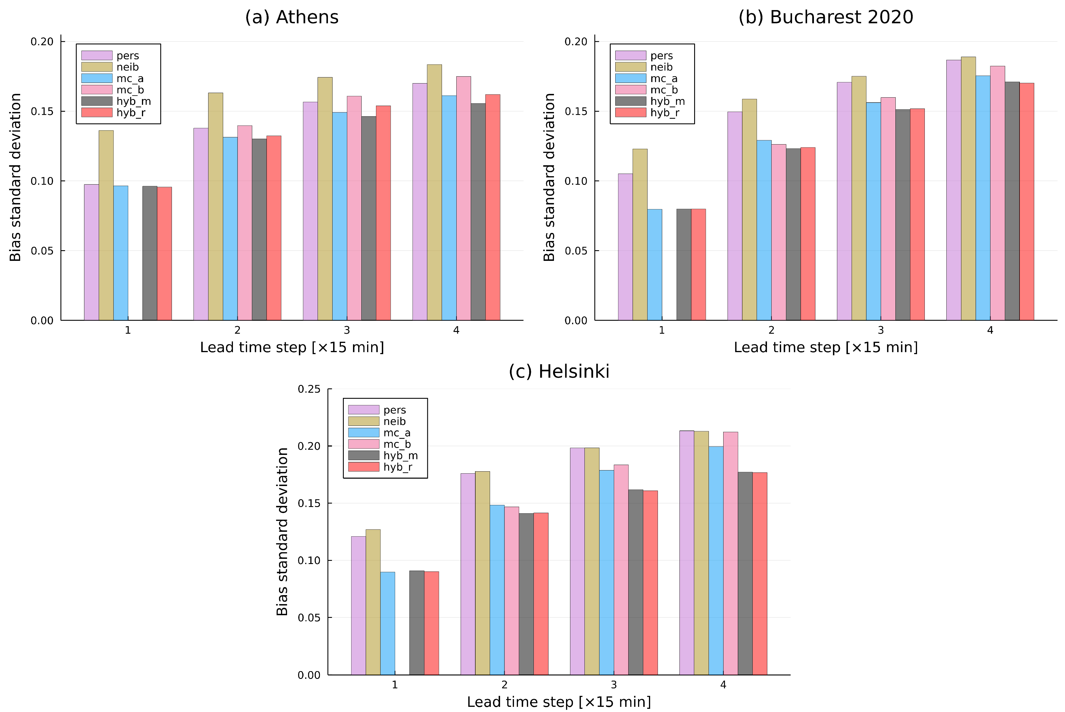
Figure A2.
Standard deviation of cloud modification factor (CMF) prediction bias for (a) Athens, (b) Bucharest, and (c) Helsinki.
Appendix A.1. Test for Time Homogeneity in the Transition Probabilities
Let
denote the number of transitions from a given state
to state
in the interval of observation
; the transition probabilities are
with
Using
, we test the first order Markov chain with 10 states, formulating the null hypothesis as the following [
25]:
where
denotes the time-independent transition probabilities and
the time-dependent ones, and
is the set of values of
for which
.
Under
the statistic
is approximately
distributed with
degrees of freedom, where
is the number of members of the set
.
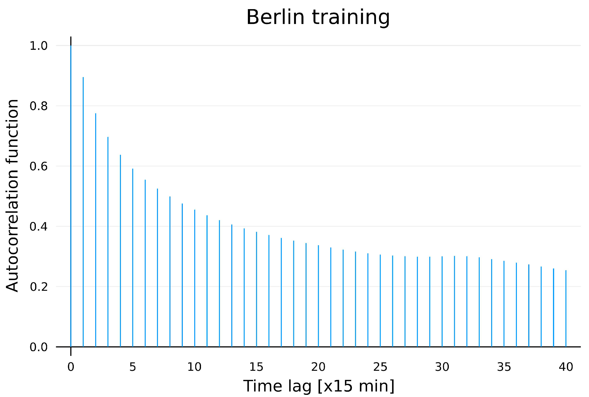
We divide the time series of the training set from 2004 to 2018 in Berlin into 4 three-month seasons, with the first season
consisting of December, January, February;
for the second season from March to May; and so on. The results of the calculated statistics for the four seasons are listed in
Table A4.
Table A4.
Test results for time homogeneity of the transition probabilities of the first order Markov chain with 10 states. The columns from left to right list the season, the sample size in each season, the degree of freedom, and the statistics, respectively.
Table A4.
Test results for time homogeneity of the transition probabilities of the first order Markov chain with 10 states. The columns from left to right list the season, the sample size in each season, the degree of freedom, and the statistics, respectively.
| t | Sample Size | DoF | Statistic |
|---|
| 1 | 45,345 | 97 | 4383.091 |
| 2 | 76,656 | 99 | 98.019 |
| 3 | 87,403 | 100 | 422.324 |
| 4 | 58,203 | 89 | 200.771 |
| sum | 267,607 | 385 | 5104.206 |
Comparing the statistics with the percentage points of the distribution, we can reject with a significance level of 5% (), thus confirming that time inhomogeneity is present for the training data set from 2004 to 2018 in Berlin. Note here the class imbalance and the distinguished different statistics among the sub-samples, especially between winter and summer.
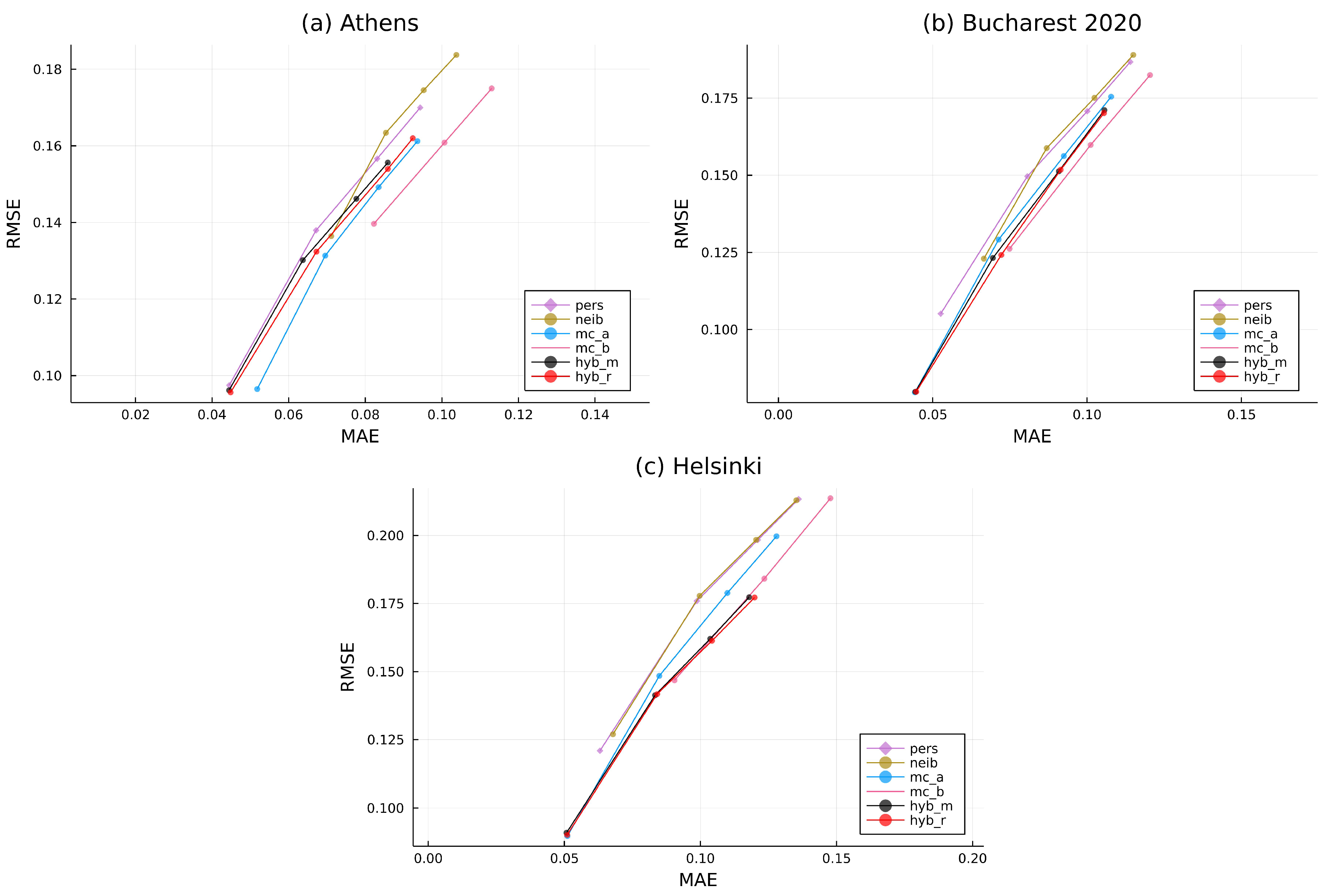
Figure A3.
Mean absolute error (MAE) verses root mean square error (RMSE) for (a) Athens, (b) Bucharest, and (c) Helsinki.
Figure A3.
Mean absolute error (MAE) verses root mean square error (RMSE) for (a) Athens, (b) Bucharest, and (c) Helsinki.
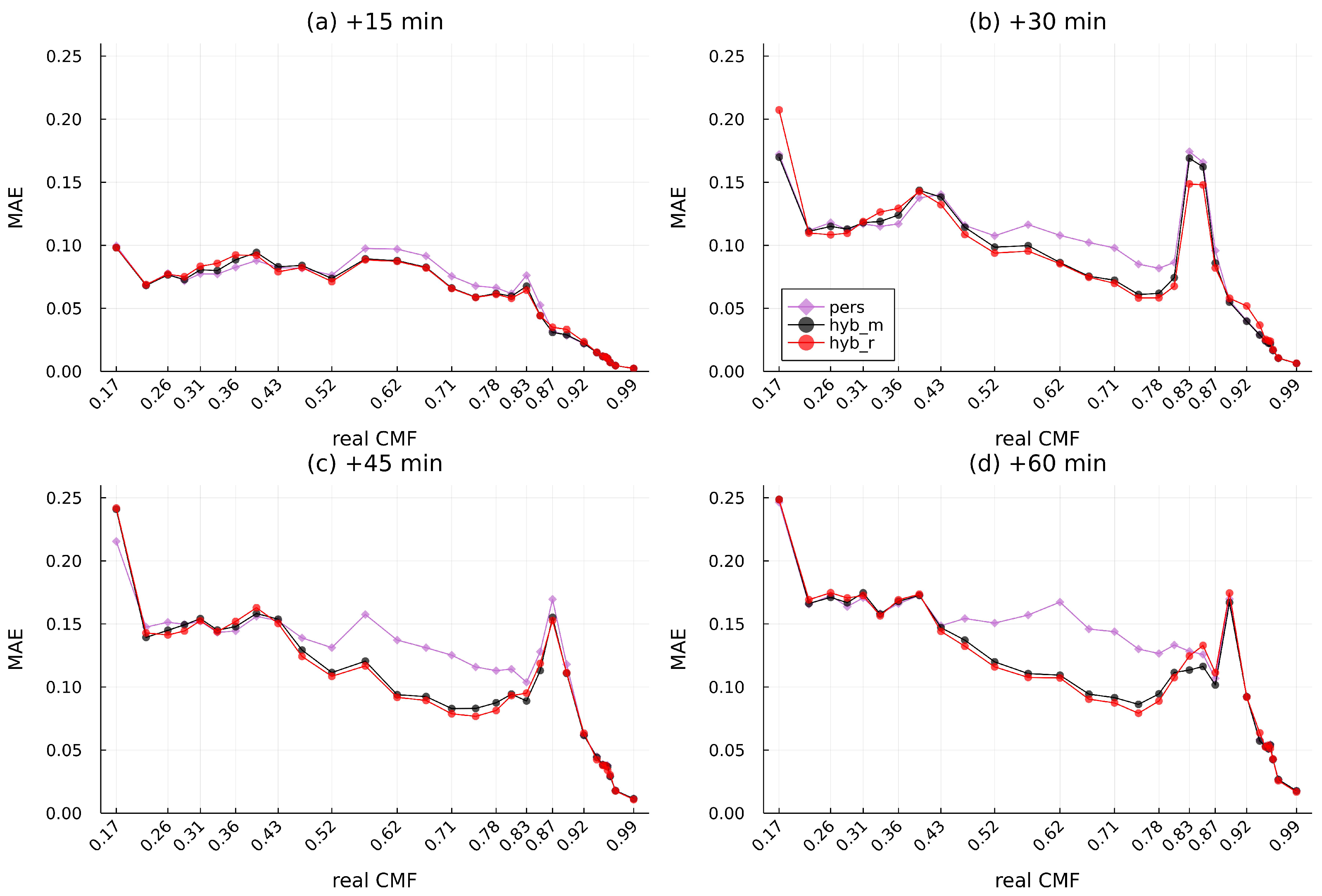
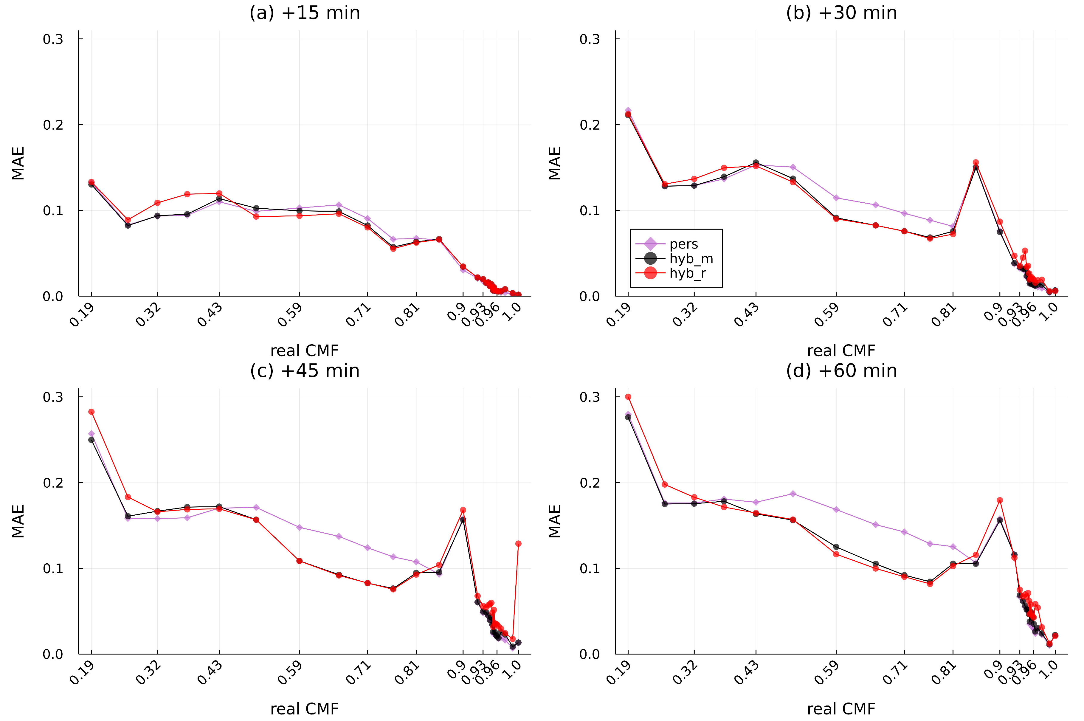
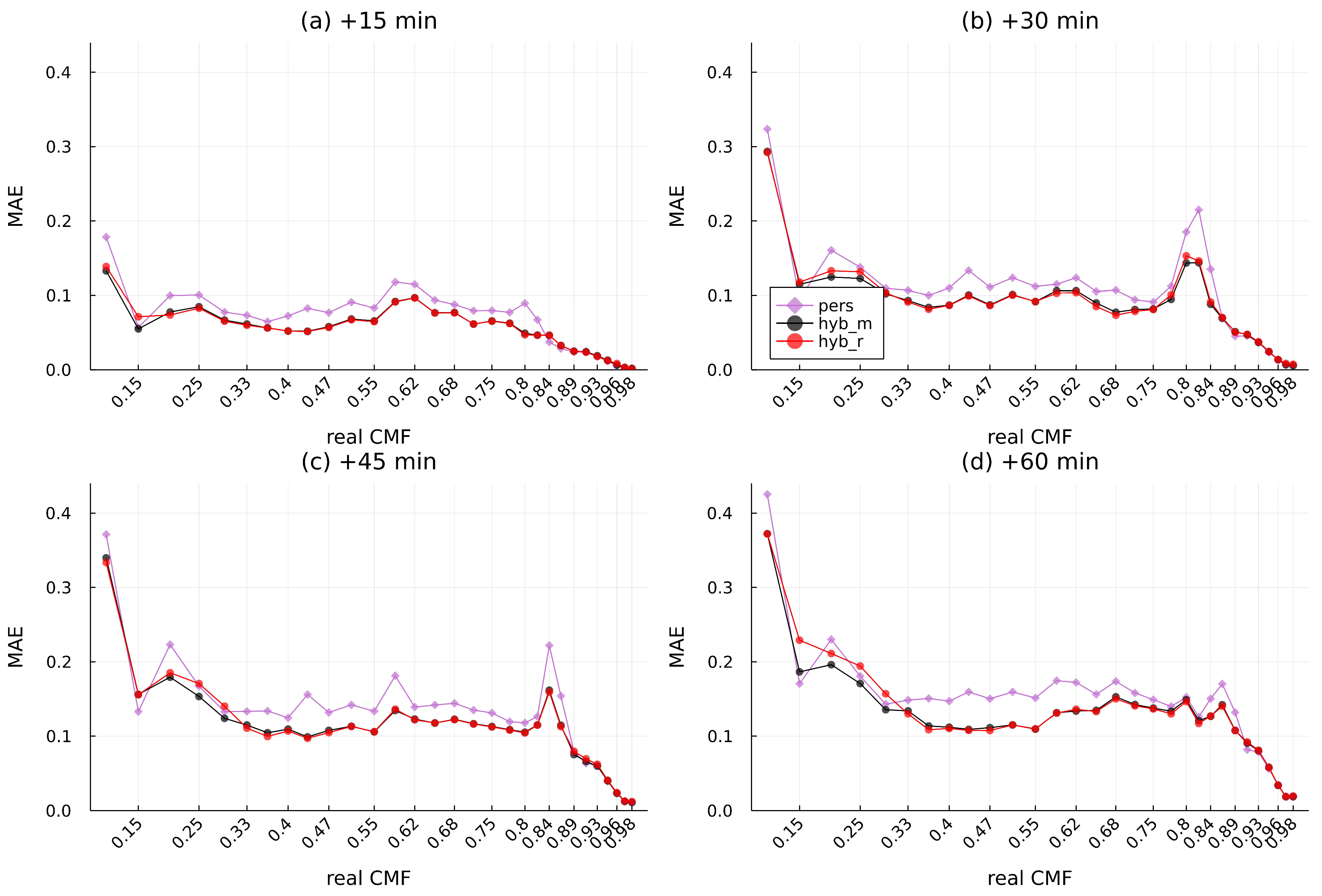
Figure A4.
MAE for each CMF class for (a) 15 min, (b) 30 min, (c) 45 min, and (d) 60 min ahead in 2020 for Athens.
Figure A4.
MAE for each CMF class for (a) 15 min, (b) 30 min, (c) 45 min, and (d) 60 min ahead in 2020 for Athens.
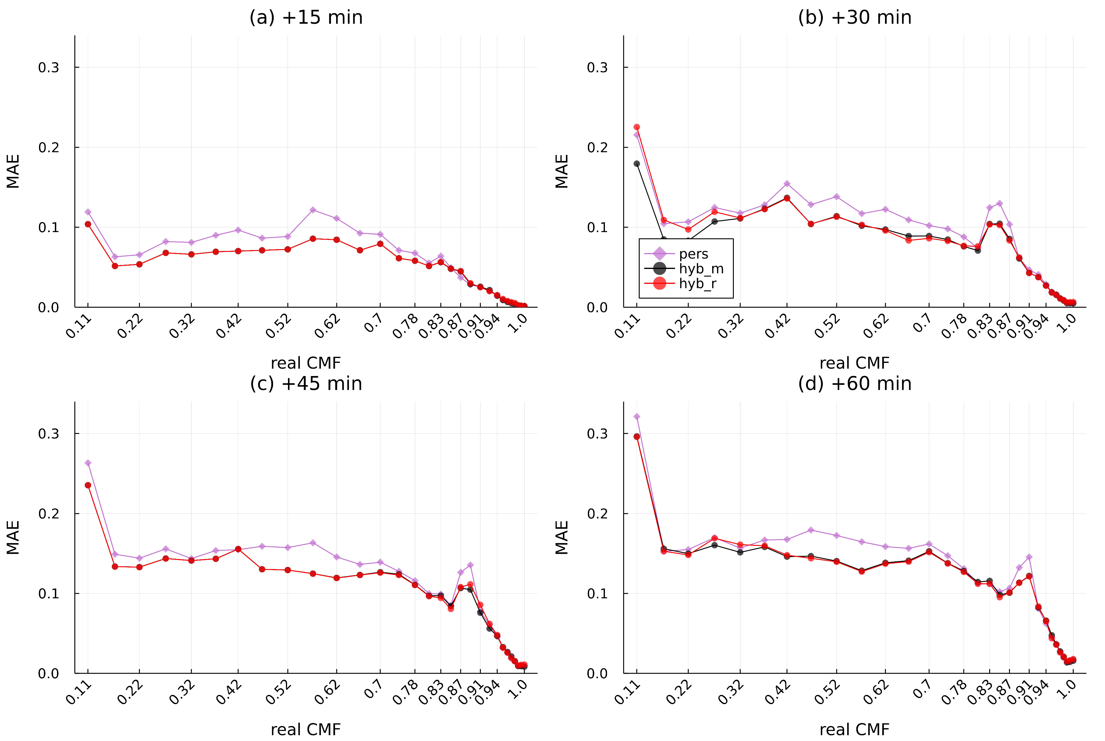
Figure A5.
MAE for each CMF class for (a) 15 min, (b) 30 min, (c) 45 min, and (d) 60 min ahead in 2020 for Bucharest.
Figure A5.
MAE for each CMF class for (a) 15 min, (b) 30 min, (c) 45 min, and (d) 60 min ahead in 2020 for Bucharest.
Figure A6.
MAE for each CMF class for (a) 15 min, (b) 30 min, (c) 45 min, and (d) 60 min ahead in 2020 for Helsinki.
Figure A6.
MAE for each CMF class for (a) 15 min, (b) 30 min, (c) 45 min, and (d) 60 min ahead in 2020 for Helsinki.
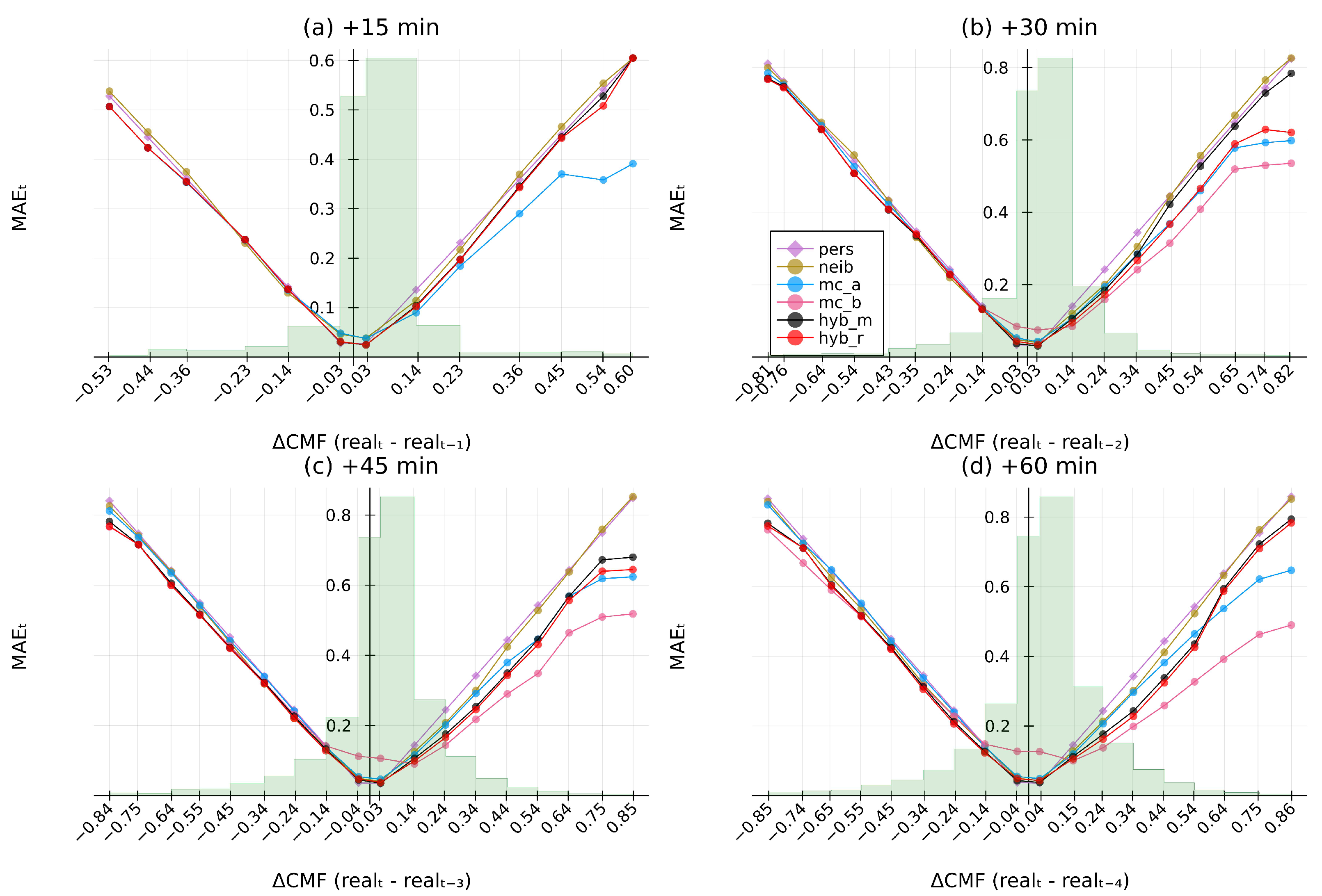
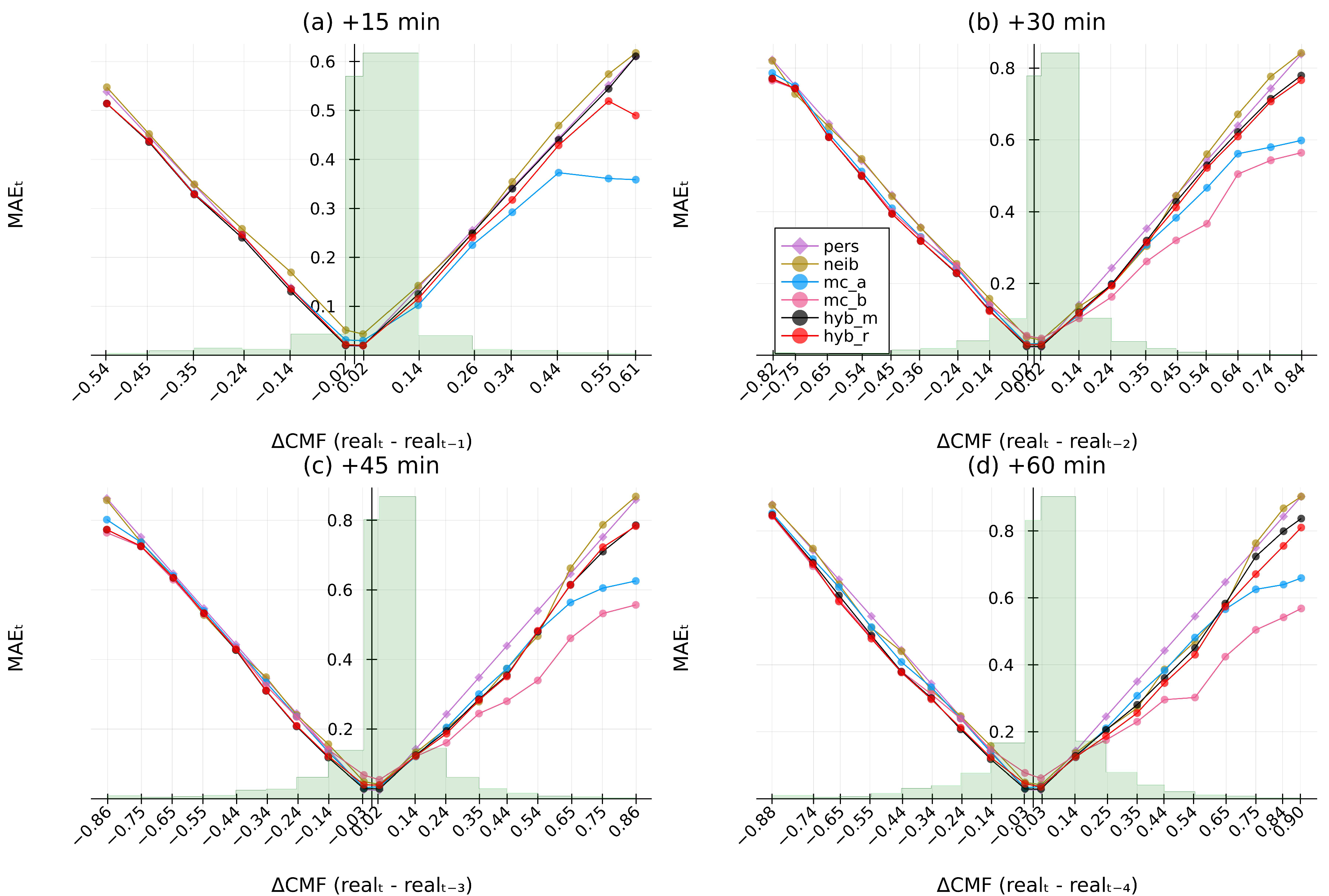
Figure A7.
MAE of CMF change for (a) 15 min, (b) 30 min, (c) 45 min, and (d) 60 min ahead for Athens.
Figure A7.
MAE of CMF change for (a) 15 min, (b) 30 min, (c) 45 min, and (d) 60 min ahead for Athens.
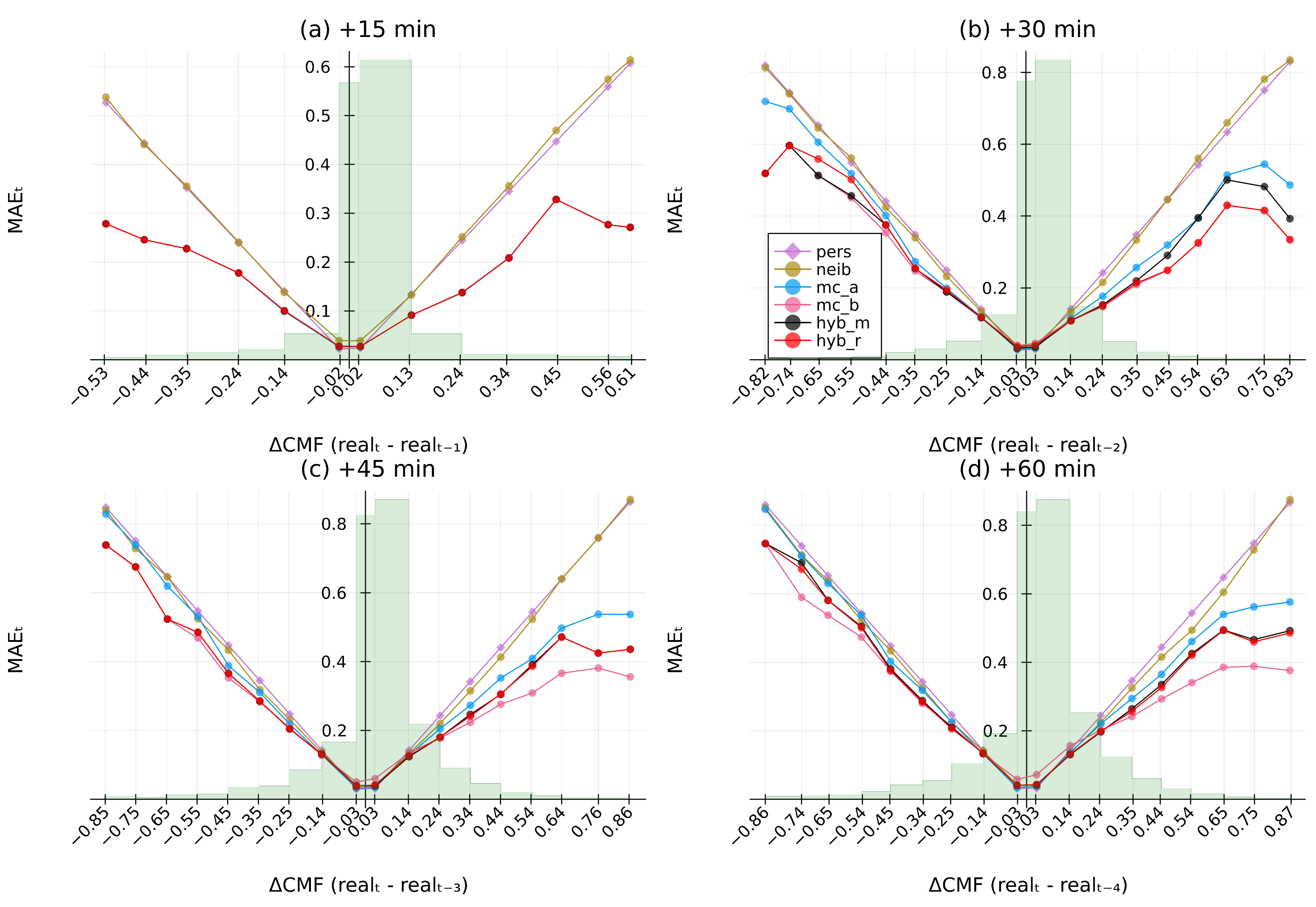
Figure A8.
MAE of CMF change for (a) 15 min, (b) 30 min, (c) 45 min, and (d) 60 min ahead for Bucharest.
Figure A8.
MAE of CMF change for (a) 15 min, (b) 30 min, (c) 45 min, and (d) 60 min ahead for Bucharest.
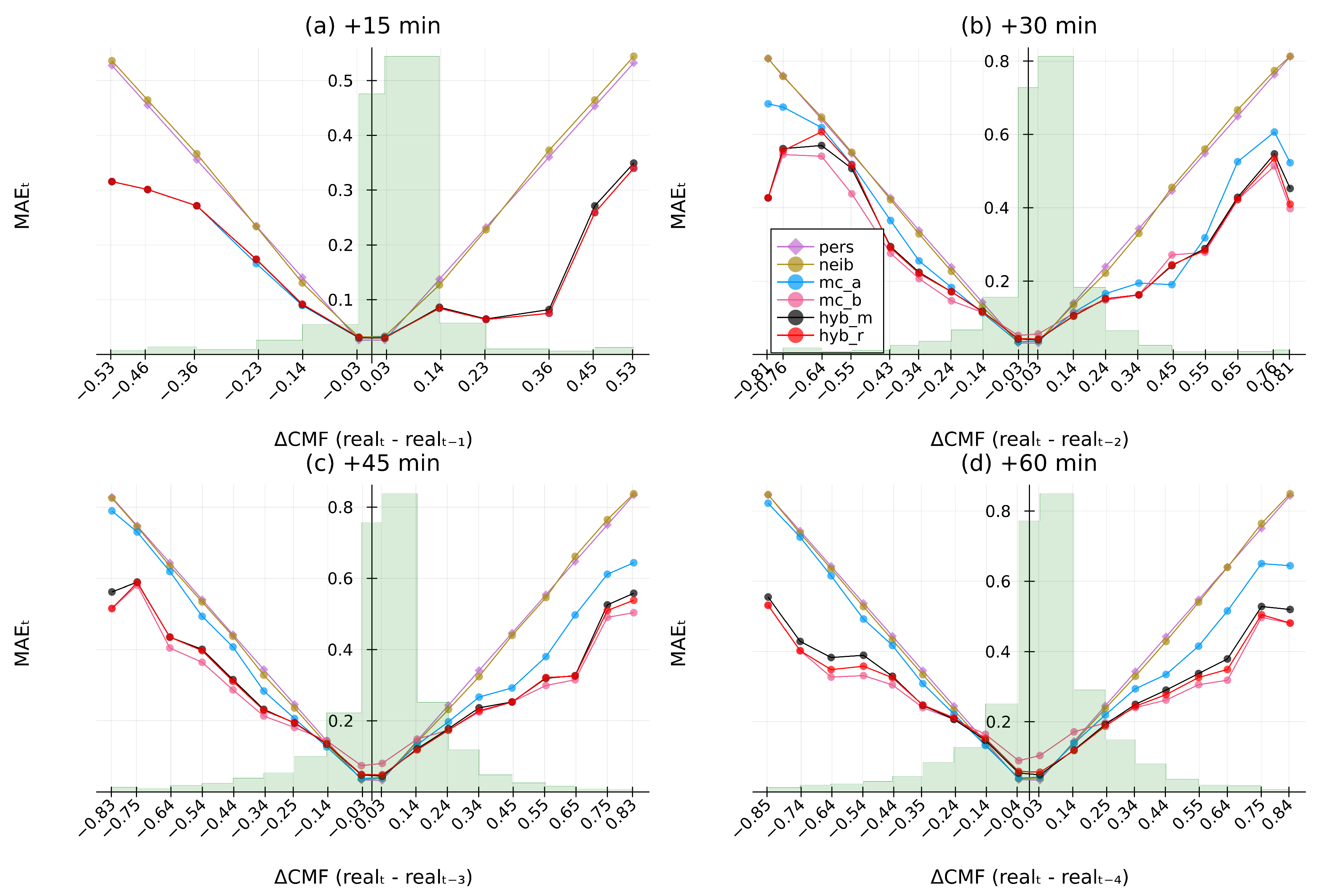
Figure A9.
MAE of CMF change for (a) 15 min, (b) 30 min, (c) 45 min, and (d) 60 min ahead for Helsinki.
Figure A9.
MAE of CMF change for (a) 15 min, (b) 30 min, (c) 45 min, and (d) 60 min ahead for Helsinki.


 ,
, 
