
Tracing and Evaluating Life-Cycle Carbon Emissions of Urban Multi-Energy Systems


Abstract
:1. Introduction
- A.
- Background
- B.
- Literature Review
- C.
- Contributions
- A tracing method is proposed to determine the life-cycle carbon emission flow among various devices in UMESs. Specifically, the carbon emission models of different devices, including energy sources and EHs, are established considering both the construction and operation phases. On this basis, the carbon flow matrixes of the EH are developed by combining the devices’ carbon emission models and the energy flow model. In this way, the distribution of life-cycle carbon emission flow in UMESs at different phases can be traced.
- Based on the traced carbon flow, two evaluation indices are proposed to analyze the carbon emissions of devices and consumers in UMESs, including the device carbon distribution factor (DCDF) and consumer carbon distribution factor (CCDF). In specific, the DCDF index is to characterize the carbon emissions per unit of energy generated by EH devices, while the CCDF index reflects the proportion of carbon emissions delivered to consumers at different phases, such as construction and operation. Through these indicators, the key devices and consumers with high carbon emissions in the system can be identified, which can guide the formulation of carbon reduction strategies.
2. Life-Cycle Carbon Emissions of UMESs
2.1. Carbon Emissions of Energy Sources
2.1.1. Construction-Produced Carbon Emissions
2.1.2. Operation-Produced Carbon Emissions
2.2. Carbon Emissions of EH Devices
2.2.1. Construction-Produced Carbon Emissions
2.2.2. Operation-Produced Carbon Emissions
3. Tracing Method to Determine Life-Cycle Carbon Emission Flow of EH
3.1. Energy Flow Model of EH
3.2. Life-Cycle Carbon Tracing Model Integrated with Energy Flow of the EH
3.2.1. Tracing Carbon Flows Related to Energy Sources
3.2.2. Tracing Construction-Produced Carbon Related to Energy Hub
4. Evaluation of Life-Cycle Carbon Emissions of UMESs
4.1. Evaluation Indices
- (1)
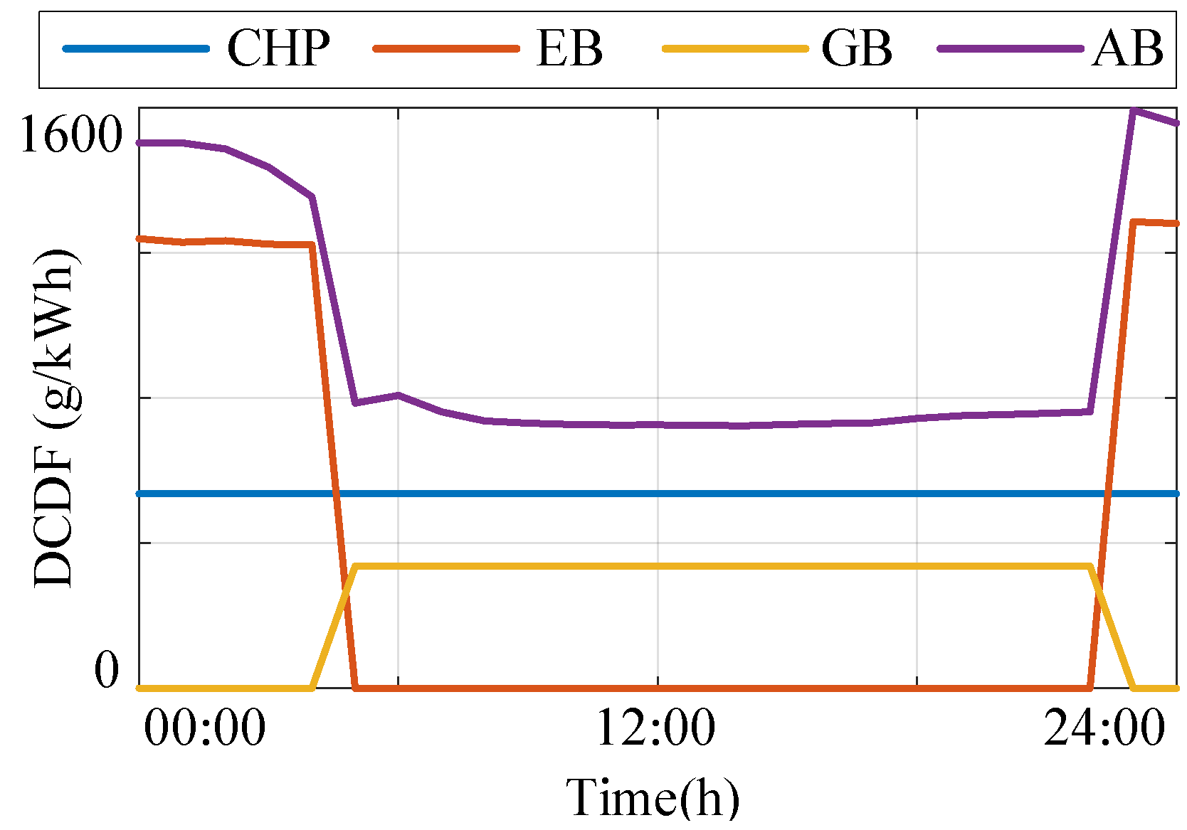
- Device Carbon Distribution Factor
- (2)
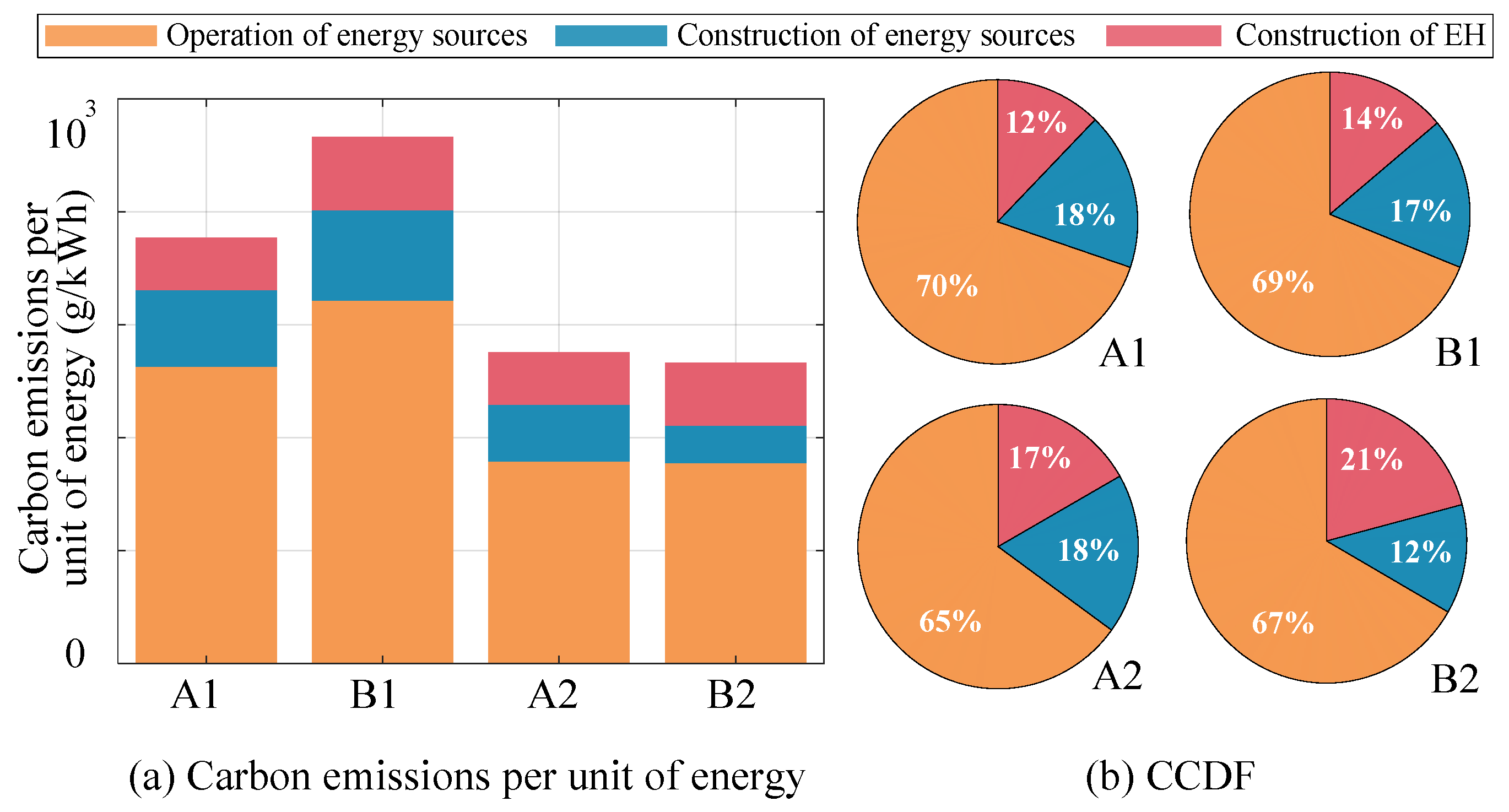
- Consumer carbon distribution factor
4.2. Evaluation Processes
- Step 1. Input life-cycle data of different power plants and gas wells. The data can include annual construction-produced and operation-produced carbon emissions per unit of energy generated by different energy sources, e.g., the annual construction-produced and operation-produced carbon emissions per unit of energy generated by thermal power plants.
- Step 2. Input life-cycle data of different devices of EH, e.g., the types of construction materials and their weight, the life-cycle carbon emissions of construction materials per kilogram, the transportation distance between purchase and construction, and the carbon emissions of transportation per kilogram per kilometer.
- Step 3. Utilize Equation (5) to calculate the amount of life-cycle carbon emissions of different EH devices during the construction phase considering different construction materials and their transportation.
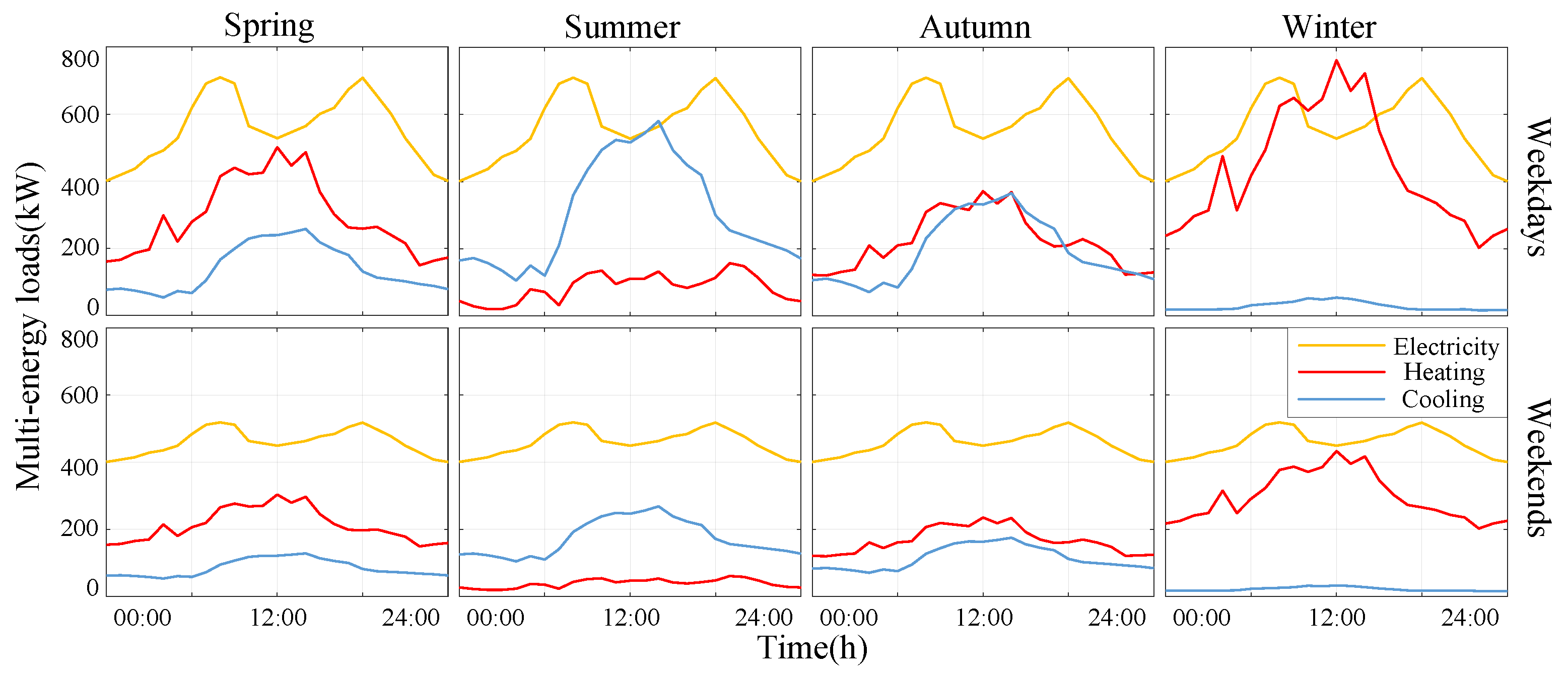
- Step 4. Input EH data, i.e., the serving time of devices, the history of energy flow on weekdays and weekends in four seasons, the output limit of devices, the ramp rate limit of devices, and the energy conversion efficiency (coefficients of performance) of devices.
- Step 5. Based on the results of Step 3 and Step 4, utilize Equation (2) to calculate the construction-produced carbon emissions per unit of energy generated by EH devices, considering the multi-energy loads’ fluctuation among weekdays and weekends in four seasons.
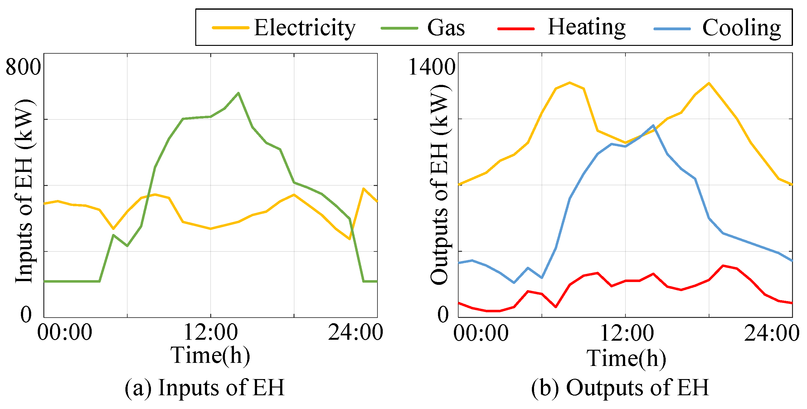
- Step 6. Utilize Equations (7)–(12) to calculate the energy flow and the outputs of devices in EH for the economy. In this step, energy conversion and energy sources costs are considered.
- Step 7. Utilize Equations (13)–(24) to calculate the carbon flow generated by different devices in UMESs. Additionally, each energy flow in UMESs consists of the operation-produced and construction-produced carbon emissions of energy sources and the construction-produced carbon emissions of EH devices, which are calculated respectively.
- Step 8. Utilize Equation (25) to calculate the DCDF index and utilize Equation (26) to calculate the CCDF index.
5. Case Studies
5.1. Test System and Parameters
5.2. Analysis Results
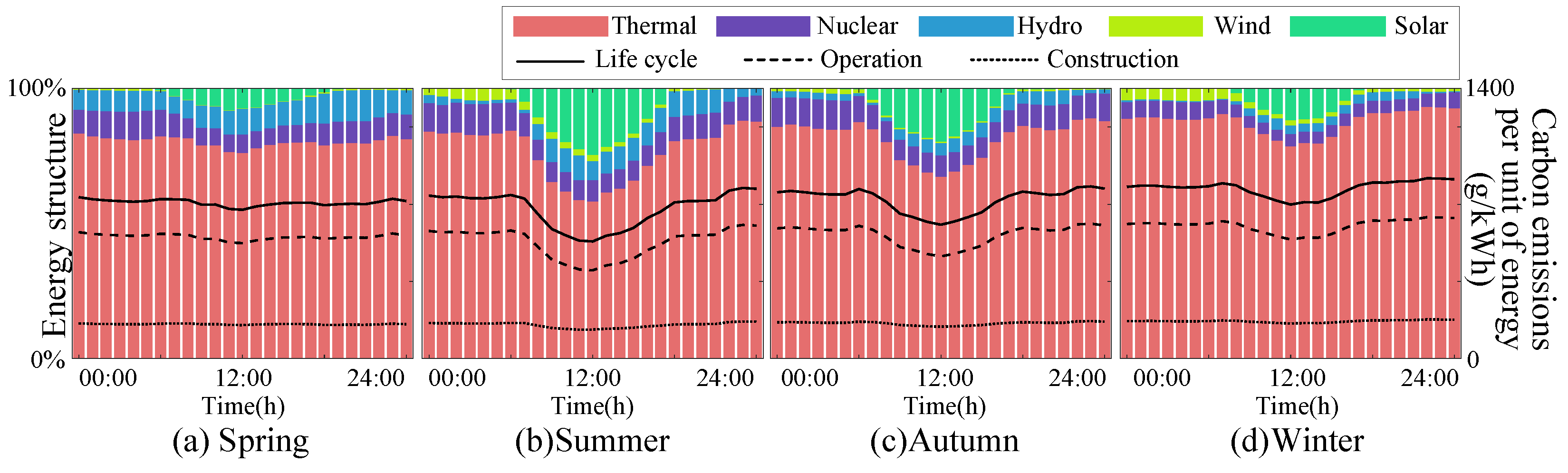
- (1)
- Carbon emissions of energy sources and EH devices
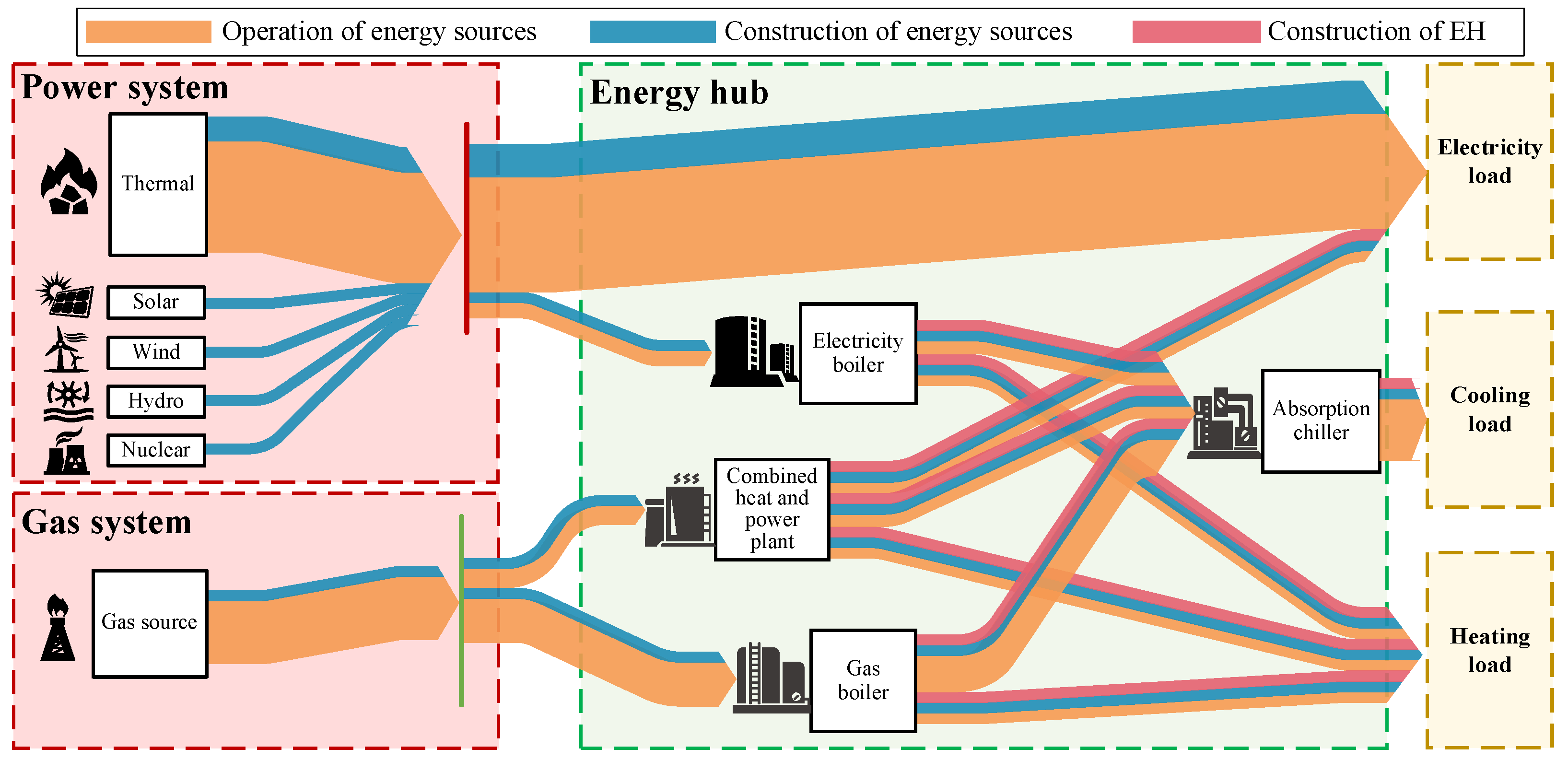
- (2)
- Carbon emission flow of the UMES
- (3)
- Evaluation indices
5.3. Discussion
6. Conclusions
Author Contributions
Funding
Institutional Review Board Statement
Informed Consent Statement
Conflicts of Interest
Appendix A
References
- Olabi, A.; Obaideen, K.; Elsaid, K.; Wilberforce, T.; Sayed, E.T.; Maghrabie, H.M.; Abdelkareem, M.A. Assessment of the pre-combustion carbon capture contribution into sustainable development goals SDGs using novel indicators. Renew. Sustain. Energy Rev. 2021, 153, 111710. [Google Scholar] [CrossRef]
- Accelerating the Transition from Coal to Clean Power. Available online: https://ukcop26.org/energy/ (accessed on 17 March 2022).
- Yang, X.; Shang, G.; Deng, X. Estimation, decomposition and reduction potential calculation of carbon emissions from urban construction land: Evidence from 30 provinces in China during 2000––2018. Environ. Dev. Sustain. 2021, 1–18. [Google Scholar] [CrossRef]
- Klüppel, H.-J. The Revision of ISO Standards 14040-3—ISO 14040: Environmental management—Life cycle assessment—Principles and framework—ISO 14044: Environmental management—Life cycle assessment—Requirements and guidelines. Int. J. Life Cycle Assess. 2005, 10, 165. [Google Scholar] [CrossRef]
- Chau, C.-K.; Leung, T.M.; Ng, W.Y. A review on Life Cycle Assessment, Life Cycle Energy Assessment and Life Cycle Carbon Emissions Assessment on buildings. Appl. Energy 2015, 143, 395–413. [Google Scholar] [CrossRef]
- Cheng, Y.; Zhang, N.; Wang, Y.; Yang, J.; Kang, C.; Xia, Q. Modeling Carbon Emission Flow in Multiple Energy Systems. IEEE Trans. Smart Grid 2019, 10, 3562–3574. [Google Scholar] [CrossRef]
- Moser, A.; Muschick, D.; Gölles, M.; Nageler, P.; Schranzhofer, H.; Mach, T.; Tugores, C.R.; Leusbrock, I.; Stark, S.; Lackner, F.; et al. A MILP-based modular energy management system for urban multi-energy systems: Performance and sensitivity analysis. Appl. Energy 2019, 261, 114342. [Google Scholar] [CrossRef]
- Gil, H.A.; Joos, G. Generalized Estimation of Average Displaced Emissions by Wind Generation. IEEE Trans. Power Syst. 2007, 22, 1035–1043. [Google Scholar] [CrossRef]
- Chicco, G.; Mancarella, P. Assessment of the greenhouse gas emissions from cogeneration and trigeneration systems. Part I: Models and indicators. Energy 2008, 33, 410–417. [Google Scholar] [CrossRef]
- Kang, C.; Zhou, T.; Chen, Q.; Xu, Q.; Xia, Q.; Ji, Z. Carbon Emission Flow in Networks. Sci. Rep. 2012, 2, 479. [Google Scholar] [CrossRef]
- Kang, C.; Zhou, T.; Chen, Q.; Wang, J.; Sun, Y.; Xia, Q.; Yan, H. Carbon Emission Flow from Generation to Demand: A Network-Based Model. IEEE Trans. Smart Grid 2015, 6, 2386–2394. [Google Scholar] [CrossRef]
- Wang, Y.; Qiu, J.; Tao, Y. Optimal Power Scheduling Using Data-Driven Carbon Emission Flow Modelling for Carbon Intensity Control. IEEE Trans. Power Syst. 2021, 1–11. [Google Scholar] [CrossRef]
- Zhang, X.; Chen, Y.; Yu, T.; Yang, B.; Qu, K.; Mao, S. Equilibrium-inspired multiagent optimizer with extreme transfer learning for decentralized optimal carbon-energy combined-flow of large-scale power systems. Appl. Energy 2017, 189, 157–176. [Google Scholar] [CrossRef]
- Wang, Y.; Qiu, J.; Tao, Y.; Zhang, X.; Wang, G. Low-carbon oriented optimal energy dispatch in coupled natural gas and electricity systems. Appl. Energy 2020, 280, 115948. [Google Scholar] [CrossRef]
- Zhao, H.; Li, B.; Lu, H.; Wang, X.; Li, H.; Guo, S.; Xue, W.; Wang, Y. Economy-environment-energy performance evaluation of CCHP microgrid system: A hybrid multi-criteria decision-making method. Energy 2021, 240, 122830. [Google Scholar] [CrossRef]
- Bahlawan, H.; Poganietz, W.-R.; Spina, P.R.; Venturini, M. Cradle-to-gate life cycle assessment of energy systems for residential applications by accounting for scaling effects. Appl. Therm. Eng. 2020, 171, 115062. [Google Scholar] [CrossRef]
- Khan, U.; Zevenhoven, R.; Tveit, T.-M. Evaluation of the Environmental Sustainability of a Stirling Cycle-Based Heat Pump Using LCA. Energies 2020, 13, 4469. [Google Scholar] [CrossRef]
- Bian, B.; Du, Z.; Zhou, K.; Huang, T.; Lv, F. Optimal Planning Method of Integrated Energy System Considering Carbon Cost from the Perspective of the Whole Life Cycle. IOP Conf. Ser. Earth Environ. Sci. 2021, 897, 012021. [Google Scholar] [CrossRef]
- Gautam, M.; Pandey, B.; Agrawal, M. Carbon Footprint of Aluminum Production: Emissions and Mitigation. In Environmental Carbon Footprints; Muthu, S.S., Ed.; Butterworth-Heinemann: Oxford, UK, 2018; Chapter 8; pp. 197–228. [Google Scholar]
- Ye, S.; Ruan, W.; Wang, S.; Zhang, C. A bi-Level equivalent model of scheduling an energy hub to provide operating reserve for power systems. In Proceedings of the 2020 Tsinghua—HUST-IET Electrical Engineering Academic Forum, Beijing, China, 10–11 May 2020; pp. 1–7. [Google Scholar]
- Kelly, K.; McManus, M.; Hammond, G. An energy and carbon life cycle assessment of industrial CHP (combined heat and power) in the context of a low carbon UK. Energy 2014, 77, 812–821. [Google Scholar] [CrossRef] [Green Version]
- Moghaddam, I.G.; Saniei, M.; Mashhour, E. A comprehensive model for self-scheduling an energy hub to supply cooling, heating and electrical demands of a building. Energy 2016, 94, 157–170. [Google Scholar] [CrossRef]
- Vaghefi, A.; Jafari, M.; Bisse, E.; Lu, Y.; Brouwer, J. Modeling and forecasting of cooling and electricity load demand. Appl. Energy 2014, 136, 186–196. [Google Scholar] [CrossRef] [Green Version]
- China Electric Power Yearbook Committee. China Electric Power Yearbook; China Electric Power Press: Beijing, China, 2020. [Google Scholar]
- Mancarella, P.; Chicco, G. Real-Time Demand Response from Energy Shifting in Distributed Multi-Generation. IEEE Trans. Smart Grid 2013, 4, 1928–1938. [Google Scholar] [CrossRef]


| Phases | Thermal | Solar | Wind | Hydro | Nuclear | Gas |
|---|---|---|---|---|---|---|
| Construction | 215.6 | 89.9 | 18 | 12.75 | 11.9 | 19 |
| Operation | 785 | 0 | 0 | 0 | 0 | 283 |
| CHP Units (kg) | EB (kg) | GB (kg) | AB (kg) | Unit Carbon Dioxide Emissions (kg/kg) [19] | |
|---|---|---|---|---|---|
| Aluminum | 0.5 | 0 | 780 | 5040 | 11.6 |
| Copper | 672.1 | 7700 | 320 | 5760 | 2.7 |
| Zinc | 0.808 | 0 | 0 | 240 | 5.19 |
| Steel | 26790.9 | 33250 | 12500 | 44400 | 1.46 |
| Polyethylene | 267.8 | 350 | 95 | 480 | 1.462 |
| 0 | 2500 | 1100 | 2100 | 900 | 500 |
| 0 | 1000 | 200 | 2500 | 200 | 2500 |
| 200 | 4500 | 0 | 3000 | 0 | 2 |
| −739.2 | 739.2 | −554.4 | 554.4 | −2000 | 2000 |
| −1250 | 1250 | −18,000 | 18,000 | −6000 | 6000 |
| CHP Units | EB | GB | AB | |
|---|---|---|---|---|
| Total construction-produced carbon emissions amount (t) | 3870 | 6388 | 2525 | 12325 |
| Total energy generation (GW) | 37 | 26 | 135 | 58 |
| Construction-produced carbon emissions per unit of energy generated (g/kWh) | 104.6 | 245.7 | 18.7 | 212.5 |
| Former Device | Operation-Produced Carbon Emissions of Energy Sources | ||||
|---|---|---|---|---|---|
| Thermal | Gas Source | Power System | Power System | Gas System | |
| Latter device | Power system | Gas system | Electricity boiler | Electricity load | Combined heat and power plant |
| Carbon emission | 8500.73 | 4488.18 | 1094.07 | 7406.65 | 1354.78 |
| Former device | Operation-produced carbon emissions of energy sources | ||||
| Gas system | Combined heat and power plant | Combined heat and power plant | Combined heat and power plant | Electricity boiler | |
| Latter device | Gas boiler | Absorption chiller | Heating load | Electricity load | Absorption chiller |
| Carbon emission | 3133.39 | 867.06 | 0 | 487.72 | 907.41 |
| Former device | Operation-produced carbon emissions of energy sources | Construction-produced carbon emissions of energy sources | |||
| Electricity boiler | Gas boiler | Gas boiler | Absorption chiller | Thermal | |
| Latter device | Heating load | Absorption chiller | Heating load | Cooling load | Power system |
| Carbon emission | 186.65 | 2578.32 | 555.07 | 4352.8 | 1898.24 |
| Former device | Construction-produced carbon emissions of energy sources | ||||
| Nuclear | Hydro | Wind | Solar | Gas source | |
| Latter device | Power system | Power system | Power system | Power system | Gas system |
| Carbon emission | 221.8 | 133.14 | 49.13 | 145.6 | 301.32 |
| Former device | Construction-produced carbon emissions of energy sources | ||||
| Power system | Power system | Gas system | Gas system | Combined heat and power plant | |
| Latter device | Electricity boiler | Electricity load | Combined heat and power plant | Gas boiler | Absorption chiller |
| Carbon emission | 303.63 | 2144.3 | 90.95 | 210.36 | 58.21 |
| Former device | Construction-produced carbon emissions of energy sources | ||||
| Combined heat and power plant | Combined heat and power plant | Electricity boiler | Electricity boiler | Gas boiler | |
| Latter device | Heating load | Electricity load | Absorption chiller | Heating load | Absorption chiller |
| Carbon emission | 0 | 32.74 | 251.84 | 51.79 | 173.1 |
| Former device | Construction-produced carbon emissions of energy sources | Construction-produced carbon emissions of EH devices | |||
| Gas boiler | Absorption chiller | Combined heat and power plant | Combined heat and power plant | Combined heat and power plant | |
| Latter device | Heating load | Cooling load | Absorption chiller | Heating load | Electricity load |
| Carbon emission | 37.26 | 483.15 | 200.36 | 0 | 150.27 |
| Former device | Construction-produced carbon emissions of EH devices | ||||
| Electricity boiler | Electricity boiler | Gas boiler | Gas boiler | Absorption chiller | |
| Latter device | Absorption chiller | Heating load | Absorption chiller | Heating load | Cooling load |
| Carbon emission | 283.67 | 58.23 | 161.8 | 34.83 | 1619.41 |
Publisher’s Note: MDPI stays neutral with regard to jurisdictional claims in published maps and institutional affiliations. |
© 2022 by the authors. Licensee MDPI, Basel, Switzerland. This article is an open access article distributed under the terms and conditions of the Creative Commons Attribution (CC BY) license (https://creativecommons.org/licenses/by/4.0/).
Share and Cite
Zhou, X.; Sang, M.; Bao, M.; Ding, Y. Tracing and Evaluating Life-Cycle Carbon Emissions of Urban Multi-Energy Systems. Energies 2022, 15, 2946. https://doi.org/10.3390/en15082946
Zhou X, Sang M, Bao M, Ding Y. Tracing and Evaluating Life-Cycle Carbon Emissions of Urban Multi-Energy Systems. Energies. 2022; 15(8):2946. https://doi.org/10.3390/en15082946
Chicago/Turabian StyleZhou, Xiaoming, Maosheng Sang, Minglei Bao, and Yi Ding. 2022. "Tracing and Evaluating Life-Cycle Carbon Emissions of Urban Multi-Energy Systems" Energies 15, no. 8: 2946. https://doi.org/10.3390/en15082946
APA StyleZhou, X., Sang, M., Bao, M., & Ding, Y. (2022). Tracing and Evaluating Life-Cycle Carbon Emissions of Urban Multi-Energy Systems. Energies, 15(8), 2946. https://doi.org/10.3390/en15082946