Article

Prediction of the Total Base Number (TBN) of Engine Oil by Means of FTIR Spectroscopy

1
Department of Quality and Safety of Industrial Products, Institute of Quality and Product Management Sciences, Cracow University of Economics, 27 Rakowicka St., 31-510 Cracow, Poland
2
Łukasiewicz Research Network—Institute for Sustainable Technologies, 6/10 Pułaskiego St., 26-600 Radom, Poland
3
Department of Statistics, College of Economics, Finance and Law, Cracow University of Economics, 27 Rakowicka St., 31-510 Cracow, Poland
*
Author to whom correspondence should be addressed.
Energies 2022, 15(8), 2809; https://doi.org/10.3390/en15082809
Submission received: 8 March 2022 / Revised: 6 April 2022 / Accepted: 9 April 2022 / Published: 12 April 2022

Abstract

:
The objective of this study is to develop a statistical model to accurately estimate the total base number (TBN) value of diesel engine oils on the basis of the Fourier transform infrared spectroscopy (FTIR) analysis. The research sample consisted of oils used in the course of 14,820 km. The samples were collected after each 1000 km and both FTIR and TBN measurements were performed. By applying the measured absorbance values, five statistical models aimed at predicting TBN values were elaborated with the use of the following information: aggregated values of measured absorbance in defined spectral ranges, extremes at wavenumbers, or the surface area of spectral bands related to the vibrations of specific molecular structures. The obtained models may be considered a continuation and an extension of previous studies of this type described in the literature on the subject. The results of the study and the analysis of the obtained data have led to the development of two models with high predictive capabilities (R2 > 0.98, RMSE < 0.5). Another model, which had the smallest number of variables in comparison to other models, had markedly lower R2 value (0.9496) and the highest RMSE (0.5596). Yet another model, where the dimensionality of the pre-processed full spectra was reduced to four aggregates through averaging, turned out to be slightly worse than the best one (R2 = 0.9728). The study contributes to a more in-depth understanding of the FTIR-based TBN prediction tools that may be readily available to all interested parties.

Graphical Abstract

1. Introduction and Theoretical Background

The reduction of the total base number (TBN) can be related to a high temperature of engine operation, high content of sulfur in fuel, excessively long intervals between oil replacements or improper oil selection [1]. The expected end results, which can be a consequence of a decrease in TBN, are a faster degradation of lubricating oil, and an increased wear of engine components [2,3,4]. There are different ways that TBN can be determined but only some of them are standardized, for example: thermometric determination according to ASTM D8045 [5], photometric determination according to ASTM D974 [6], and potentiometric determination according to ASTM D664 [7].
The loss of operational properties can occur at different rates [8,9,10,11]. Although the TBN parameter is very informative, it fails to provide the precise value at which it is advisable to replace the oil. Vasanthan et al. [10] claims that the threshold value of TBN is 5, and below it the lubricating oil should be treated as compromised and not be used any longer. Vasanthan’s view is partly supported by Sharma and Chawla as well as Kral et al. [11,12]. They even recommended more stringent levels, claiming that engine oil fit for use has a limited base number 2–5 mg KOH/g. Chawla and Sharma [12] took different point of view and provided a relative decision rule that oil needs to be changed as soon as its TBN falls to 50% of the original (initial) level. In turn, Kral et al. [11] adopted another maximum allowed value, stating that 30% limits for each oil change should be used. Wolak [13] verified the direction and intensity of changes in the TBN of engine oils and confirmed a rapid decrease in TBN during engine use. Based on the achieved results, the author presented the model, which can be applied for predicting engine oil behavior (TBN change) during its use.
Total base number is one of the most significant parameters in the assessment of the quality of engine oils; consequently, there has been a gradual increase in new scientific articles related to the oil quality on the basis of TBN change [14,15,16]. This parameter is very often used in research describing the behavior of used engine oils throughout their service life [17,18,19,20,21]. Sharma et al. [12] attempted to model and predict the rate of TBN reduction in a diesel oil engine. Their goal was to model the TBN depletion rate, constant for specific system variables. The authors reached the conclusion that determination of mathematical models is particularly problematic for the TBN depletion rate, due to the complexity of the physiochemical changes in the oil. Robinson et al. [22] tested a sample of 80 oils with duplicate TBN values to establish criteria used in measurements. These oils were sourced from many producers, different engines, and with differing grades, and were not limited to the specific usage. Dyson et al. [23] demonstrated that TBN varies exponentially with time and introduced an equation which takes into consideration engine type, operating conditions, fuel type, and oil type. Kauffman [24] draws attention to the voltammetric method, which—according to the authors—is suitable for the analysis of both TBN and TAN (Total Acid Number). However, they concluded that the approach seems to be influenced by several variables and, as such, the research needs to be familiar with the formulation of the oils being analyzed, especially the antioxidants and their types, as these affect the results considerably.
Bassbasi et al. [25] suggested an infrared spectroscopy in order to observe and control as well as perform a fast examination of used engine oils. The infrared spectroscopy (IR) spectra provide information about the presence of specific bonds and groups in the chemical structure of the examined samples. The location of the bands in the spectrum is related to the vibration of chemical structures after absorption of infrared radiation with a characteristic wavelength [26]. The Fourier transform infrared spectroscopy (FTIR) is an indispensable method for identifying functional groups and other elements of a compound structure [27,28,29,30]. A large amount of information that is carried by the FTIR spectrum and a relatively short test time enable the effective use of this technique to monitor various oil properties, such as oxidation, nitration, and sulfonation of in-service engine oils [31,32,33,34]. Chimeno-Trinchet et al. suggested to support the analysis of ATR-FTIR information by Artificial Neural Networks (ANN) as well as Linear Discriminant Analysis (LDA). The methodology proposed by them increases the level of correct identification of deterioration degree of oils.
In their paper, Taghizaderh and D’Souza used a new approach to describe the activity of antioxidants in oil relative to TBN values; the new approach was based on the FTIR spectroscopy (method designed to measure the quantity of active base and not the total base in a medium with a polarity similar to that of petroleum-based engine oils) [35]. The study findings demonstrated that the FTIR values correlated well with the TBN values for fresh oils; however, lower correlations were found for used engine oils [35]. The authors stressed that their method is not applicable to oils containing caroboxylated ingredients (e.g., synthetic oils), as they interfere with the signal used for the quantification of the active antioxidants [35]. Dong et al. [36] expanded the FTIR spectroscopic method of rapidly and quantitatively determining the total base number (TBN) of hydrocarbon lubricating oils by spectroscopical measurement of the COO functional group of the salt that formed when trifluoroacetic acid (TFA) reacts with basic ingredients present in an oil. Sejkorova et al. claim that models using a principal component regression (PCR) does not show satisfactory results [37]. In their opinion, the most satisfactory results of calibration are obtained using the partial least squares (PLS) algorithm applied to a classic spectral record in a zone of wavenumbers 4000–650 cm−1. Nagy et al. indicated that TBN shows collinearity with oxidation and iron content with both residual ZDDP content and soot loading and this information is indirectly contained in the FTIR spectra [33]. They concluded that based on simple FT-IR spectra, no further oil analyses, e.g., TBN titrations, are required, and the “loss of information” is minimal, as most conventional parameters are indirectly contained in the FT-IR spectra.
The use of chemical methods for the determination of TBN is very time consuming, capital intensive (reagents), and harmful to the environment (hazardous solvents, such as toluene, chloroform, acetic acid, and others) [35]. Dong et al. [36] also agree with the time-consuming and labor-intensive nature of the analysis and add that a major drawback is the need for substantial volumes of organic solvents and corrosive reagents that are hazardous and difficult to dispose. Besides the environmental aspect, Macian et al. have addressed the problem of different analytical methodologies that may be applied [38]. It is not entirely correct to compare such studies, as the response of each of the methodologies (potentiometric determination; photometric determination) is different, which implies the need to study the new method of evaluation of TBN. Beyond these issues, there are other disadvantages such as poor sensitivity at low TBNs and a difficulty in determining visual endpoints in sooty oils. Even with automated potentiometric titration versions of the ASTM methods, the analysis is still time-consuming and cumbersome. Taghizaderh and D’Souza also pointed out that as the behavior of the antioxidant and/or titrants are strongly affected by the titration solvent in use, the TBN values obtained by two different methods are not comparable [35]. In addition, titration is carried out in a solvent mixture that has much higher polarity than the actual engine oil; therefore, the acid–base interaction is somewhat different from that encountered under operating conditions [35]. An alternative procedure to all of the mentioned determinations and methodologies is to employ mathematical methodologies based on the FTIR.
This is why the aim of this study is to determine the mathematical model that estimates the TBN value of engine oils on the basis of the FTIR spectra analysis. The study is expected to contribute to an understanding of the FTIR-based TBN tool that may be readily available to all interested parties.

2. Materials and Methods

2.1. Research Material

The research material comprised several samples of engine oil in the viscosity class SAE 5W-30 and the quality ACEA 2016—C3, API—SN, BMW longlife-04 TWIN POWER TURBO. The level of changes in the properties of the oil was thoroughly assessed. The engine oil tested was used in the BMW model 520 (2006 production year), equipped with a 1995 cm3 diesel engine and filled up each time with the fuel of the same manufacturer.
The general specification of the selected car’s model is aggregated in Table 1.
Before starting the operation, the output parameters for the sample of unused (fresh) engine oil was determined, and then the same test cycle was carried out after each 1000 km (approximately) for the entire duration of the oil’s in-service life (14,820 km) (details in Table 2). There was only one oil refill applied after the 13th collection of the samples. All of the samples were collected by using a pressure syringe through a bayonet opening, in compliance with a strictly defined procedure (running the engine for 5 min, collecting of 30 mL of sample, checking the oil level on the dipstick, and making refills of new oil if necessary).
When analyzing the obtained results, it should be taken into account that the vehicle was operated in 10–30% of time in the urban cycle and in 70–90% in the non-urban cycle. Table 2 presents the details related to the operation of the vehicle using the engine oil tested.
When analyzing the data in Table 2 in more detail, it is worth emphasizing that a total of 14 oil samples were taken during the operational period. Each subsequent collection took place on average after about 33 days. The shortest period was 13 days (Sample 4), and the longest was 82 days (Sample 9). The first control collection of the sample took place after 13 km, while each subsequent sample had a mileage increased by the number of km in the range 941–1439. Each subsequent oil sample was taken when the car covered an average of about 1060 km.

2.2. Research Methodology

The FTIR spectra were obtained with the use of the Thermo Nikolet iS10 apparatus (mid-infrared KBr beamsplitter, fast recovery deuterated triglycine sulfate (DTGS) as detector type). The transmission technique was used (the cuvette used for the tests is the ICL SL-15 ZnSe, 0.1 mm), under the following conditions: spectral region 650–4000 cm−1, spectral resolution 0.5 cm−1, and number of scans—64 differential spectra were used to analyze the chemical changes in engine oils. The recorded FTIR spectra were subjected to arithmetic processing that led to obtaining a differential spectrum as a result of subtracting the spectrum of SMP 0 (fresh oil) from the spectrum of each subsequent sample of in-service oil. The obtained differential spectra were further processed by removing the range of spectral artifacts, occurring in the ranges: 1451 cm−1 to 1474 cm−1 and from 2837 cm−1 to 2979 cm−1. Then, the recorded differential spectra were transformed into an alphanumeric form, which assigned an absorbance value to each wavenumber value. For example, in the analyzed spectral range from 650 cm−1 to 1000 cm−1, a total of 700 different absorbance values corresponding to individual wavenumbers were recorded (that is, the independent variables in the spectral plot/diagram—the spectra were recorded with a resolution of 0.5 cm−1). Thus, a set of values was obtained that were used to calculate the arithmetic mean of the absorbance values in each of the spectrum ranges selected for analysis. The calculated arithmetic means were then applied as the parameters in the statistical modeling. The arithmetic means of the absorbance were determined in the following spectral ranges: 650 ÷ 1000 cm−1, 1000 ÷ 1450 cm−1, 1475 ÷ 1800 cm−1, 1800 ÷ 2830 cm−1, and 2975 ÷ 4000 cm−1. In the above spectral ranges, changes in the intensity of individual spectral bands or changes in the position of the baseline were observed in a specific spectral range, in which there were no functional group bands, and which resulted from chemical changes in in-service engine oils during use. Hence, the calculation of the arithmetic mean of the absorbance in the analyzed range makes it possible to determine the index of global chemical changes that affect the operating parameters of the engine oil, including the total base number. The TBN value was obtained by potentiometric titration with hydrochloric acid, using the Mettler Toledo DL 20 automatic titration kit. This method complies with the ASTM D4739 standard.

3. Results

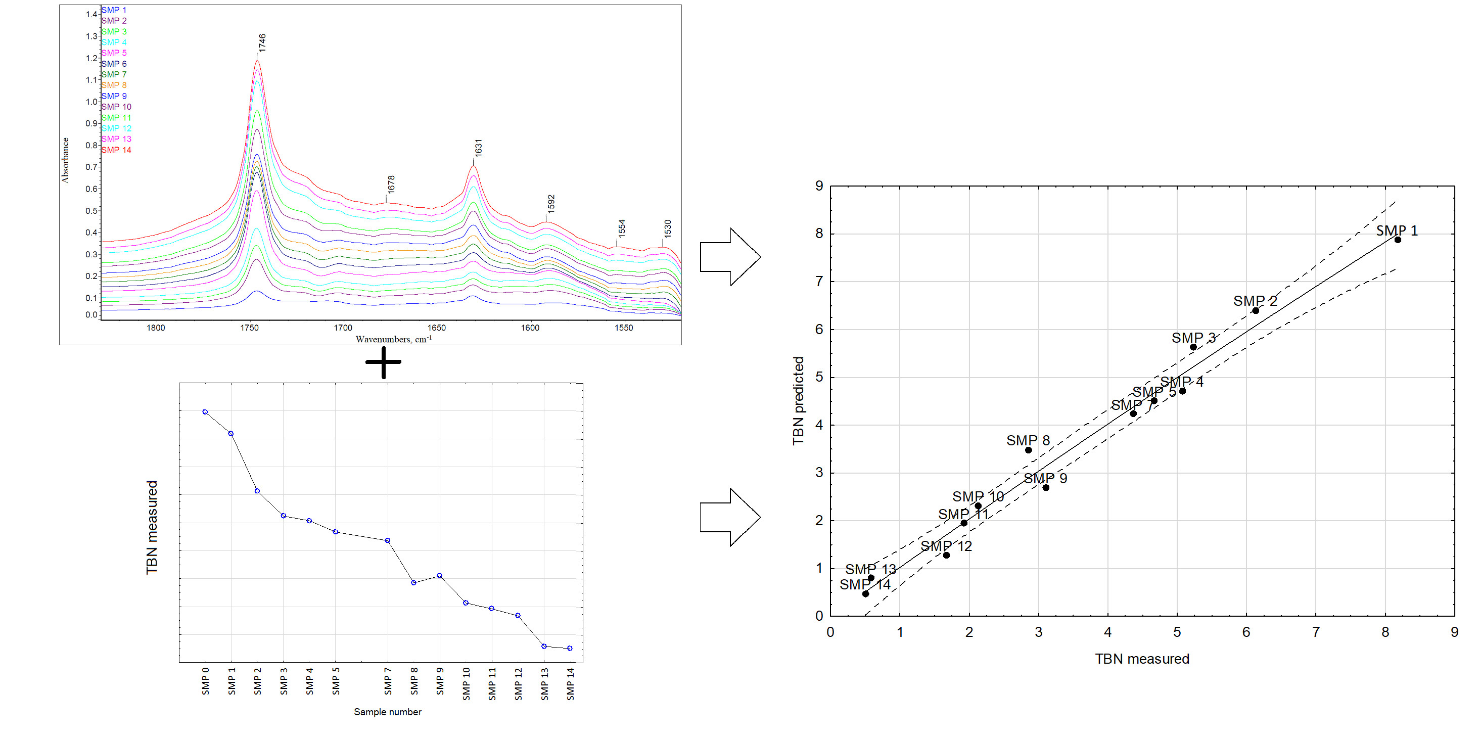
3.1. The FTIR Results

The chemical character of the new and used engine oils was explored by analyzing their FTIR spectra. The changes in the particular absorbance bands were determined based on the differential spectra. The variations of FTIR spectra of the collected samples are depicted below (Figure 1).
The obtained differential spectra have noise in the wavenumber ranges 2837–2979 cm−1 and 1451–1474 cm−1, where there are valence bands of C-H bonds in hydrocarbon structures. This area is not removed, so as not to confuse the reader. The remaining spectral areas are characterized by an increase in the position of the baseline (1800–2830 cm−1 and 2975–4000 cm−1) or characterized by a change in the spectral signal intensity of organosulfur structures (1000–1450 cm−1) and structures of oxygengroups or nitrogroups (1475–1800 cm−1). The spectral range from 650 cm−1 to 1000 cm−1 is the dactyloscopic range, characteristic for each organic compound. Various chemical compounds present in the oils cause fluctuations in the differential spectra.
Most information about chemical transformations in engine oils, taking place during their operation, is carried by, and can be found, in the spectral ranges in which the changes in the intensity of spectral bands are observed. In particular, the spectrum range from 1800 to 1475 cm−1 (Figure 2), in which there are signals that can be associated with organic-oxygen products and oil nitration products. These products of oil deterioration are acidic and therefore reduce the TBN.
An example of such band is the signal observed at the wavenumber of 1631 cm−1, which corresponds to the asymmetric bending vibrations of the NO2 group in aromatic nitro compounds. Nevertheless, a signal at the wavenumber of 1554 cm−1 is also observed, which may be related to the vibrations of the R-NO2 structure in nitroalkanes. The nitro compounds are slightly acidic due to the possible formation of a tautomeric acid structure. Thus, it should be assumed that an increase in the amount of oxidation products and nitration products leads directly to a reduction in the alkaline reserve, so it is possible to correlate the amount of such products with the total base number of the oil.
Another band from the discussed spectral range is the signal at the wavenumber of 1746 cm−1, which is related to the vibrations of the carbonyl groups present in esters. As shown in Figure 3, the intensity of this band gradually increases, which can be observed in the spectrum of each successive sample tested, proportionally rising with the number of kilometers traveled (understood as the engine oil service life). The relationship shows a linear upward trend.
The second significant spectral region is the wavenumber range from 1450 to 1000 cm−1, in which there are bands related to sulfur additions—those that improve lubricity, but also those that increase the alkaline reserve and disperse solid products (an example of such an additive can be basic calcium sulfonate). The summary of spectra observed in this area is presented in Figure 4.
In this range (1450 to 1000 cm−1), there are signals coming from sulfone additives, which decrease during oil use, and also from aromatic sulfonation products, which are formed during chemical changes taking place in the oil during its operation. For example, the vibrations of the structure S=O are represented by a band at the wavenumber of 1062 cm−1. Moreover, the following wavenumber vibrations can be associated with sulfones or sulfonates: 1169 cm−1 and 1196 cm−1 as well as 1326 cm−1 and 1339 cm−1. The analyzed range also includes the vibration band of the C-O-C structure, present in ester products found in engine oils, and located at the wavenumber of 1020 cm−1. Therefore, the absorbance averaging procedure in a specific spectral range, which was applied during statistical modeling, seems fully justified, as it reflects the resultant chemical changes.
The ongoing aging processes of engine oils lead to the formation of complex chemical compounds, the infrared spectra of which have many signals in the so-called a fingerprint region. In turn, the spectral range below 1000 cm−1 is an area that carries little information in terms of the direct interpretation of the chemical structure of the compounds formed. However, in this area there are bands related to the vibrations of aromatic rings, of substituents in these rings, or long hydrocarbon chains, that is, compounds that take part in the formation of nitro and ester substances or intermediate compounds associated with the reactions of radical destruction and oxidation of broken long hydrocarbon chains. For example, in the spectral range from 870 cm−1 to 690 cm−1, signals related to aromatic nitro compounds as well as long chain hydrocarbons containing more than five carbon atoms in the chain may appear. Thus, this area can also be taken into account during statistical modeling using the averaged absorbance value from this spectral area as a component of the developed model. The characterized chemical changes lead to the formation of compounds that also raise the background of the entire spectrum and, accordingly, its baseline, which may be related, for example, to the generation of dark resin products or, in some cases, even soot. It should be noted that soot means not only the presence of carbon, but also of functional groups found on its surface, including oxygen groups, with the acidic properties. Changes in the position of the baseline are especially observed in the following spectral ranges: from 1800 cm−1 to 2837 cm−1, and also from 2979 cm−1 to 4000 cm−1.

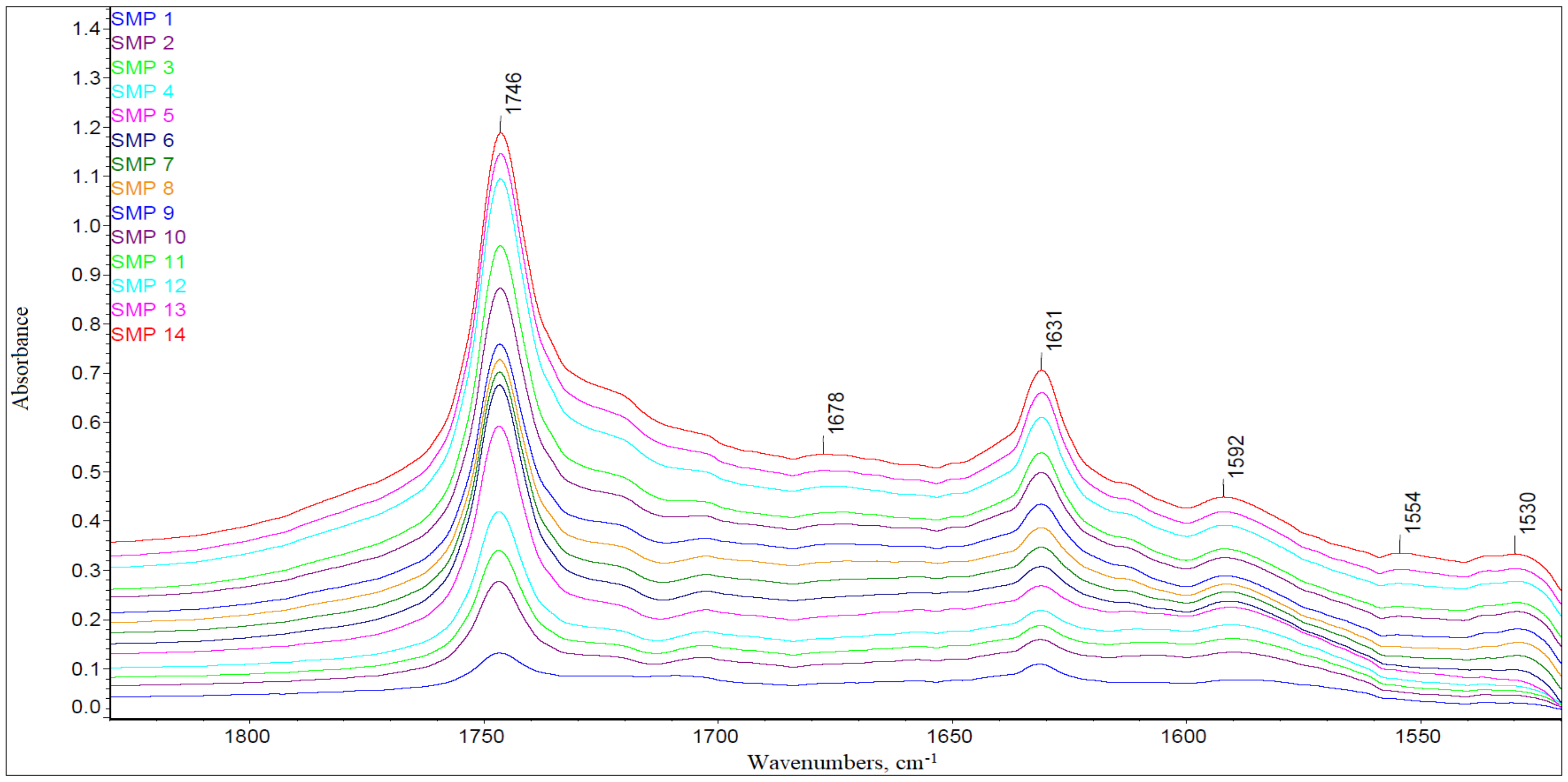
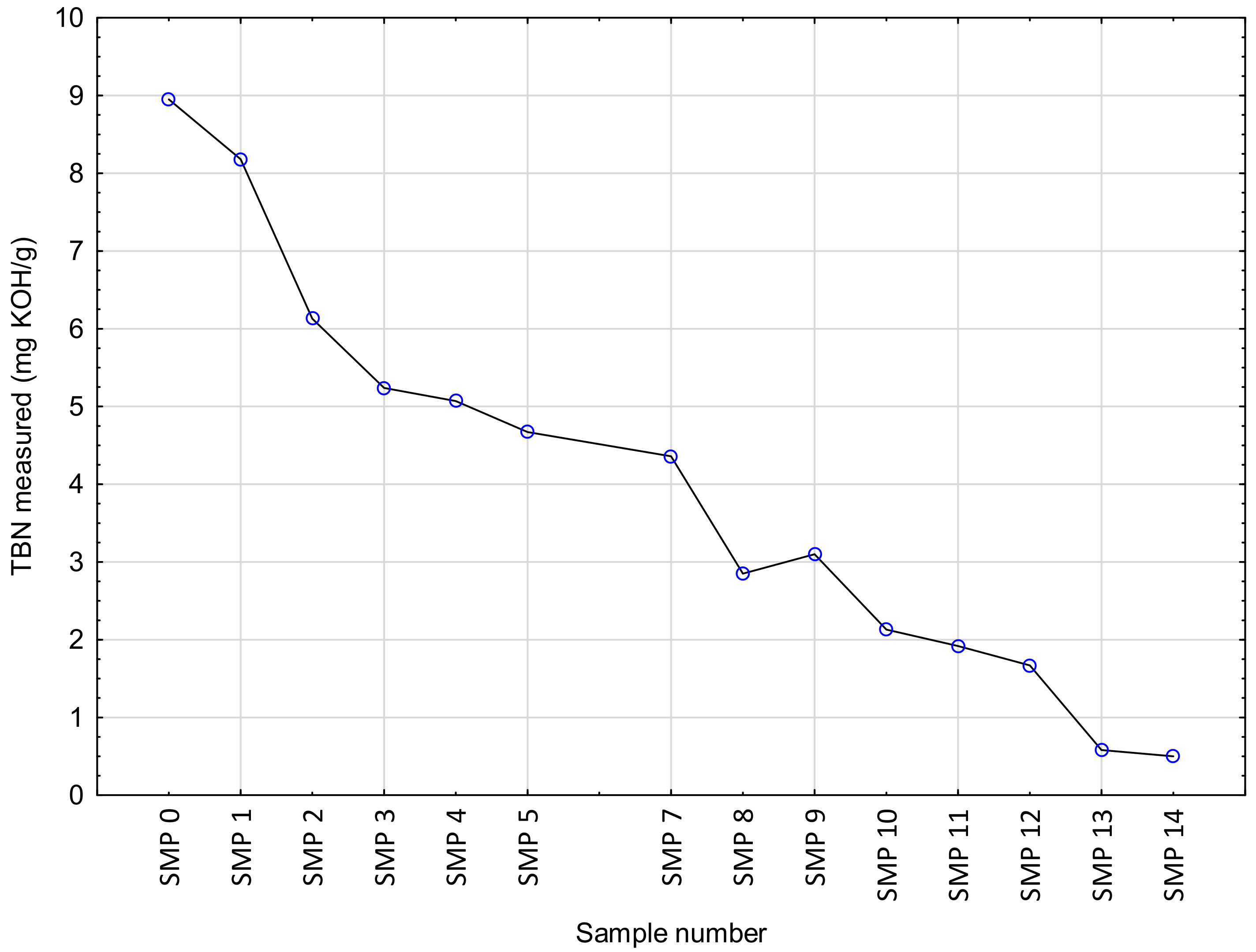
3.2. The TBN Results

The changes of the total base number (TBN) of the tested engine oil had an almost linear trend (Figure 5).
A fast loss of alkali reserve (the capacity of a lubricating oil to neutralize acid combustion products) was observed, resulting in a rapid decrease in the total base number. The starting level of TBN was 8.18 mg KOH/g and at the end of the test the TBN was on the level of 0.50 mg KOH/g. By far the greatest decrease in the TBN value was recorded after the first thousand kilometers of operation (specifically after 1144 km—SMP 2)—by 2.05 mg KOH/g. The second significant decrease in the value was identified for the SMP 8—TBN decreased by 1.51 mg KOH/g in relation to the previous sample. When analyzing the percentage changes, it should be indicated that the largest one was noted for the SMP 13 (after 13,521 km)—the TBN value compared to the sample from the previous measurement point (SMP 12) decreased by 65%. Other substantial decreases in TBN were observed for the SMP 8 in relation to the SMP 7–35%—the SMP 10 in relation to the SMP 9–31% and the SMP 2 in relation to the SMP 1–25%. The remaining samples exhibited a percentage change in the range of 3–14%. However, in one case there was an increase in the value of TBN, for the SMP 9 in relation to the SMP 8—the TBN increased by 8%. Detailed percentage changes for individual samples are presented in Table 2. Sample no. 6 (SMP 6), for which the TBN value was 7.08 mg KOH/g, was removed from further analyzes, because it was found that the sample was taken without conducting the sampling procedure, i.e., the engine was not started before sampling for a minimum of 5 min, as was restricted in the case of other samples. A heterogeneous sample was taken through the bayonet and the results distorted the course of all TBN degradation. The decrease in the alkaline reserve along with the engine oil service life (and the number of kilometers traveled) is related to the decrease in the number of enriching additives that raise the TBN (e.g., a basic calcium sulfonate with the structure as shown in Figure 6), which is the result of the neutralization reaction of the acid products of thermo-oxidation of the oil.
The comparison of changes in the TBN value with the intensity of spectral bands demonstrates that it is possible to link the TBN index with the content of nitration products (band at 1631 cm−1), and organic–oxygen products of oil aging (band at 1746 cm−1), which are acidic, as well as with an average content of sulfonic compounds (band at 1169 cm−1), which are both additives with dispersing and washing properties that increase the alkaline reserve, and the products of sulfonation occur in in-service oils during use. These relationships can be initially observed when analyzing the results presented in Table 3. This provides the basis for an attempt at statistical modeling, which can make it possible to determine the relationship between these parameters.
The percentage changes in TBN and the intensity of the selected signals presented in Table 3 were calculated based on the nominal values, corresponding to the sample from the previous measurement point. The baseline values necessary for calculating the percent changes for the SMP 2 are the results obtained for the SMP 1 (and so forth). The fluctuations between the results, illustrating the changes in the intensity of bands in the oil sample spectra, may indicate the overlapping of bands in certain spectral ranges, originating from various chemical compounds but having the same functional groups. Therefore, an effect of averaging the spectral signal may be observed, coming from the substances with a similar chemical structure and products of concurrent chemical reactions, e.g., the neutralization of sulfone additives, increasing the alkaline reserve and the simultaneous sulfonation reaction of aromatic products formed during the operation of the engine oil. Considering the above, an attempt was made to determine the correlation between the averaged absorbances in the selected ranges of the spectrum or the surface areas of the selected spectral bands with the TBN values, which would facilitate the elaboration of a mathematical tool for a rapid assessment of the base number on the basis of the global analysis of the FTIR spectrum.

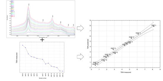
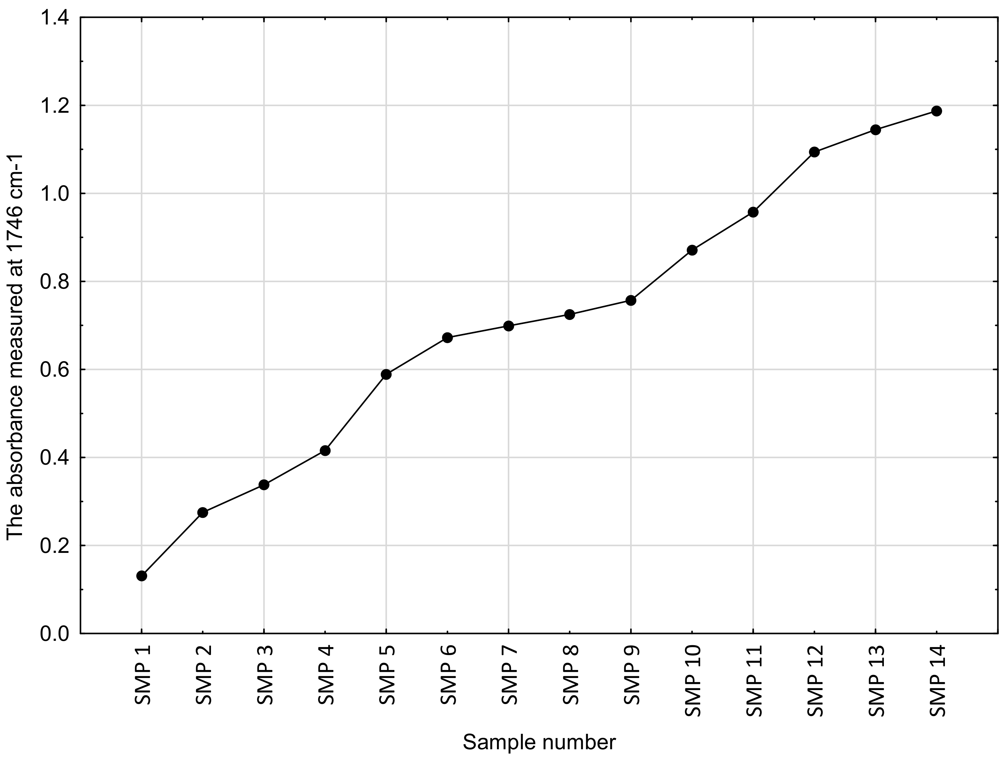
4. Modeling TBN Levels Based on the FTIR Spectra

The available subject literature has revealed that some attempts at modeling the relation between the FTIR spectra and the TBN levels have already been undertaken [37,38]. As shown in Macian’s et al. work [38], the quality of TBN predictions was similar across many different modeling approaches. More sophisticated models did not reveal any meaningful prediction improvements in comparison to the simpler models. Taking these findings into account, and while faced with the small sample size, it was decided that in this study only modestly parameterized models should be fitted to the data. To that end, a multiple linear regression model was estimated by employing the least squares method. The analysis was performed with the use of R software, version 4.0.3. [39].
The pre-processing of the FTIR spectra was performed in line with the previous studies [37,38]. One of the more common pre-treatment processes when using the FTIR spectra is to subtract the spectrum of the fresh engine oil from the spectrum of the target sample. Other possibility is to apply the first or second derivatives to subtract the background effect. However, Macian et al. [38] reported that these procedures can be affected by the problem of fixing the background line and it is not always advisable to perform them. As a result, these steps were not included in the study. However, the pre-processing included the removal of outliers, as some relatively narrow FTIR bands (1451–1474 cm−1 and 2837–2979 cm−1) had the abnormal noises, i.e., they were thoroughly covered with fine, very narrow, and uniform-looking unevenness. In differential spectra, these are typical effects of subtracting output spectra on the border of the spectral range of functional groups and the fingerprint region of the spectrum. There are many overlapping signals in this region, the position of which depends on the chemical environment of the vibrating molecular structure of a given chemical compound. In particular, there may be signals of valence vibrations of the aromatic ring, vibrations of the plane deformation groups -CH3 and -CH2, as well as valence vibrations of the asymmetric NO2 group, or the carboxylate anion. Due to the complex chemical processes taking place during the operation of engine oil, the chemical structure of the compounds formed may be slightly different in each sample. That is why subtracting the FTIR spectra of these samples at specific frequencies may yield a noise-generating result. Nevertheless, this range of the FTIR spectrum is not critical for identifying chemical changes in the oil, and in some studies, it is even automatically deleted using the spectrum editing and processing software.
Aggregated values of measured absorbance in defined spectral ranges, extremes at wavelengths, or the surface area of spectral bands related to vibrations of specific molecular structures were used as explanatory variables to determine statistical models. Using the measured absorbance values, the following five models were developed:
  • Model A—the model was built on the basis of average absorbance values calculated in four wavenumber ranges of the same width, i.e., <1000 cm−1, 1000–2000 cm−1, 2000–3000 cm−1, and >3000 cm−1.
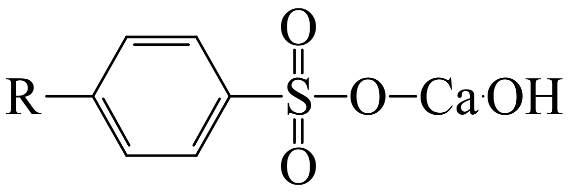
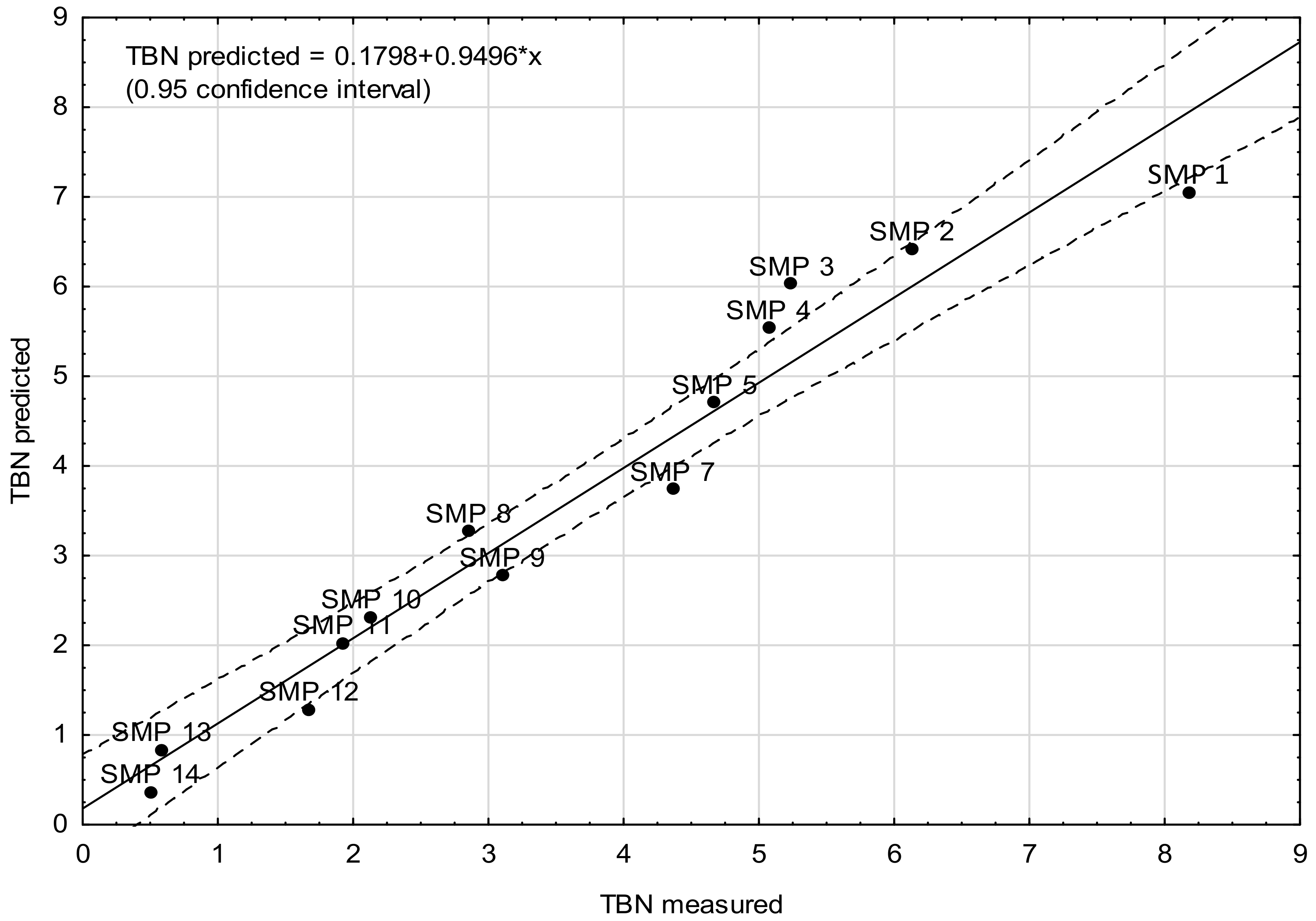
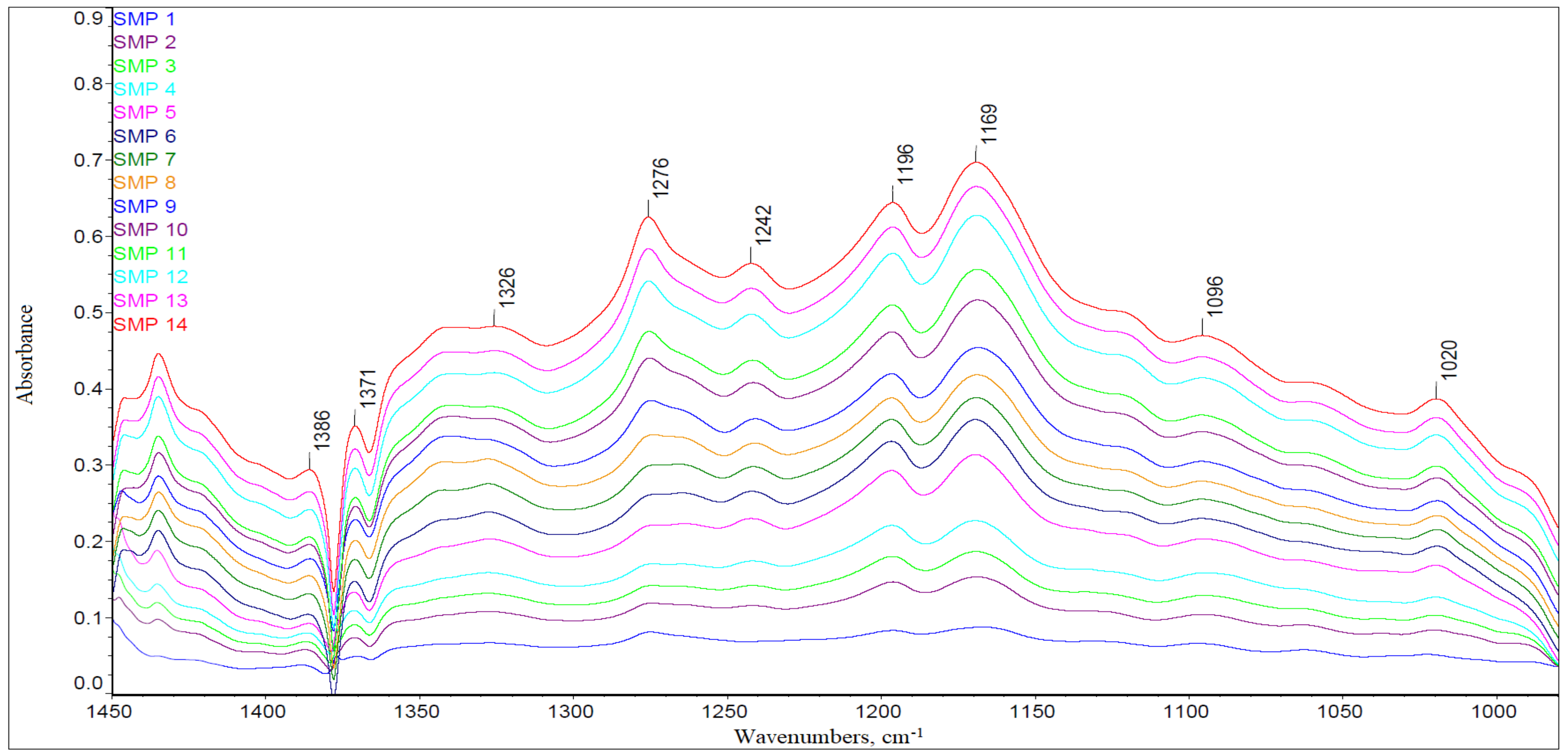
  • Model B—the model was elaborated on the basis of average absorbance values in two key wavenumber ranges, i.e., 1000–1450 cm−1 and 1470–1800 cm−1, in which the greatest differences in the intensity of spectral bands could be identified, related to the changes in the chemical structure of engine oil components as a result of operational aging processes. In the 1800 to 1475 cm−1 range, there are signals related to organic-oxygen products as well as oil nitration products, which are all acidic and thus reduce the alkaline reserve by reactions with additives increasing the alkaline reserve, which eventually leads to their depletion (an increase in the amount of oxidation products causes a decrease in the alkaline reserve). In the range of 1450 to 1000 cm−1, bands related to sulfur additives can be observed, those that improve lubricity, but also those that increase the alkaline reserve and disperse solids (an example of such an additive can be the basic calcium sulfonate). In this range, therefore, there are signals coming from sulfone additives, which gradually decrease during the operation of engine oil. Moreover, the bands of aromatic sulfonation products, which are formed during oil use, are also found in this range.
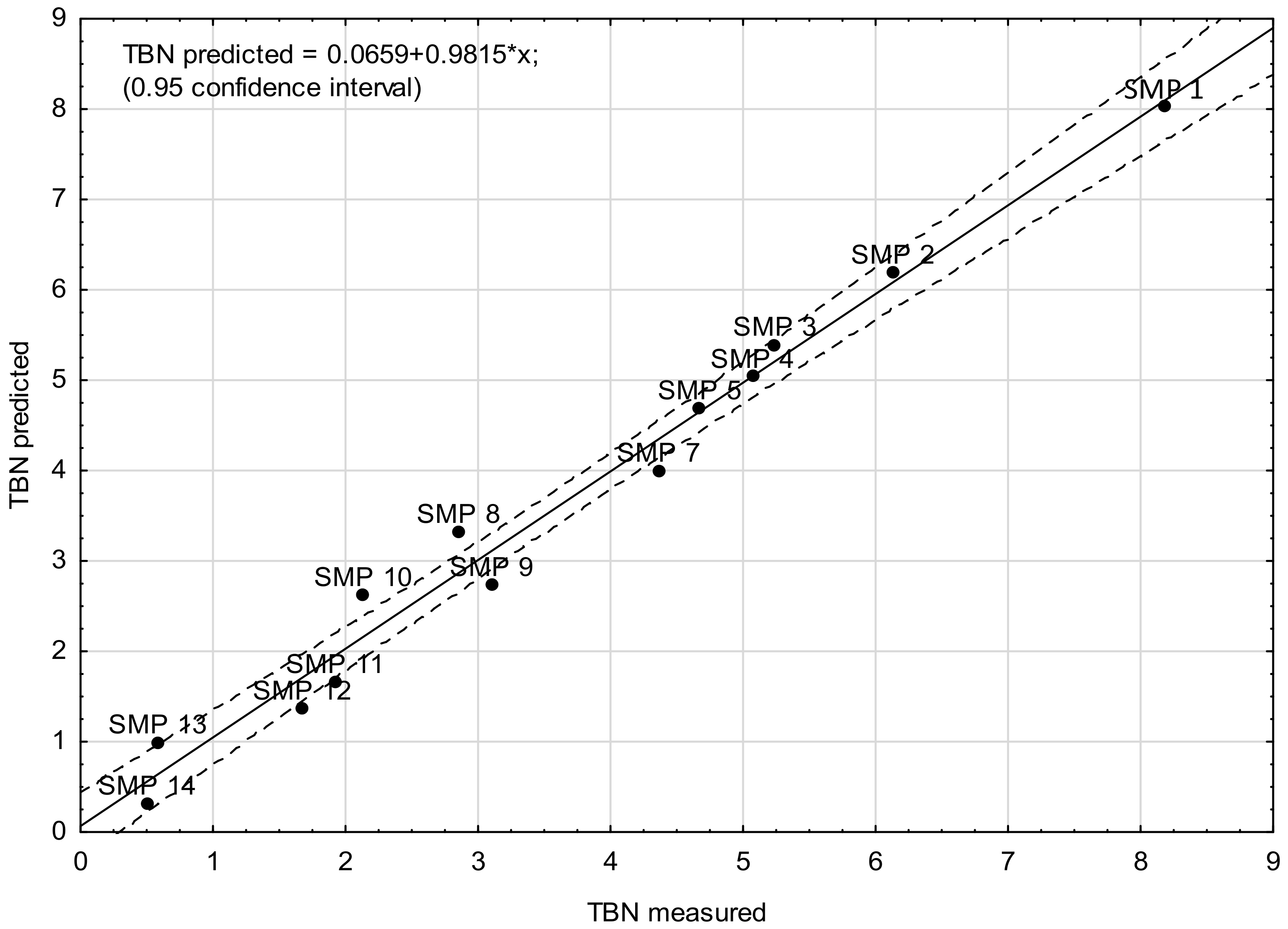
  • Model C—the model was determined on the basis of mean absorbance values calculated in five wavenumber ranges, i.e., <1000 cm−1, 1000–1450 cm−1, 1475–1800 cm−1, 1800–2830 cm−1, and 2975–4000 cm−1. The indicated wavenumber ranges help identify any structural changes in the chemical structure of engine oil and the changes in background intensity. What is more, the fingerprint region of the spectrum below 1000 cm−1 was analyzed separately. As mentioned above, the calculations did not take into account the noise ranges occurring as a result of the generation of the differential spectrum.
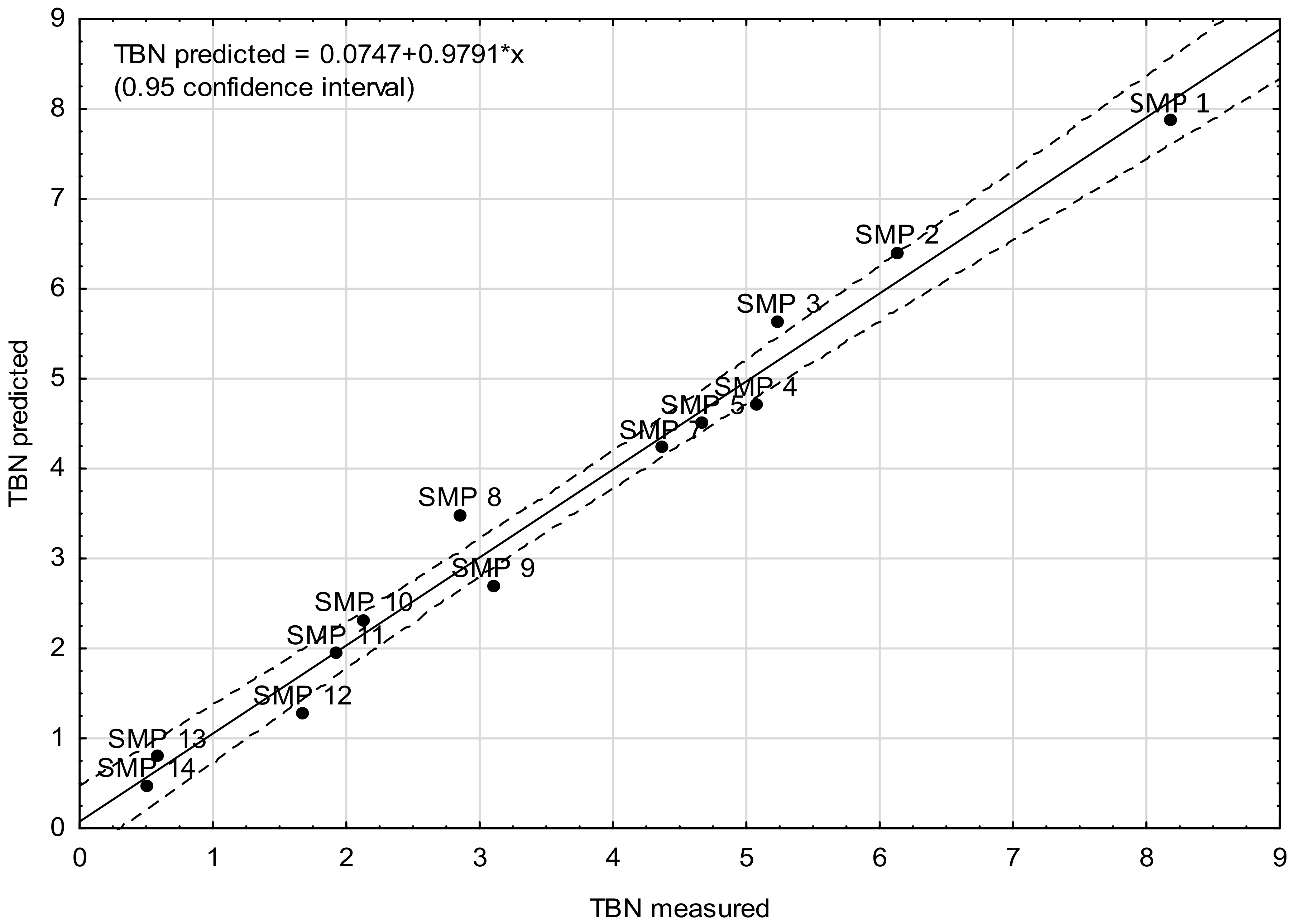
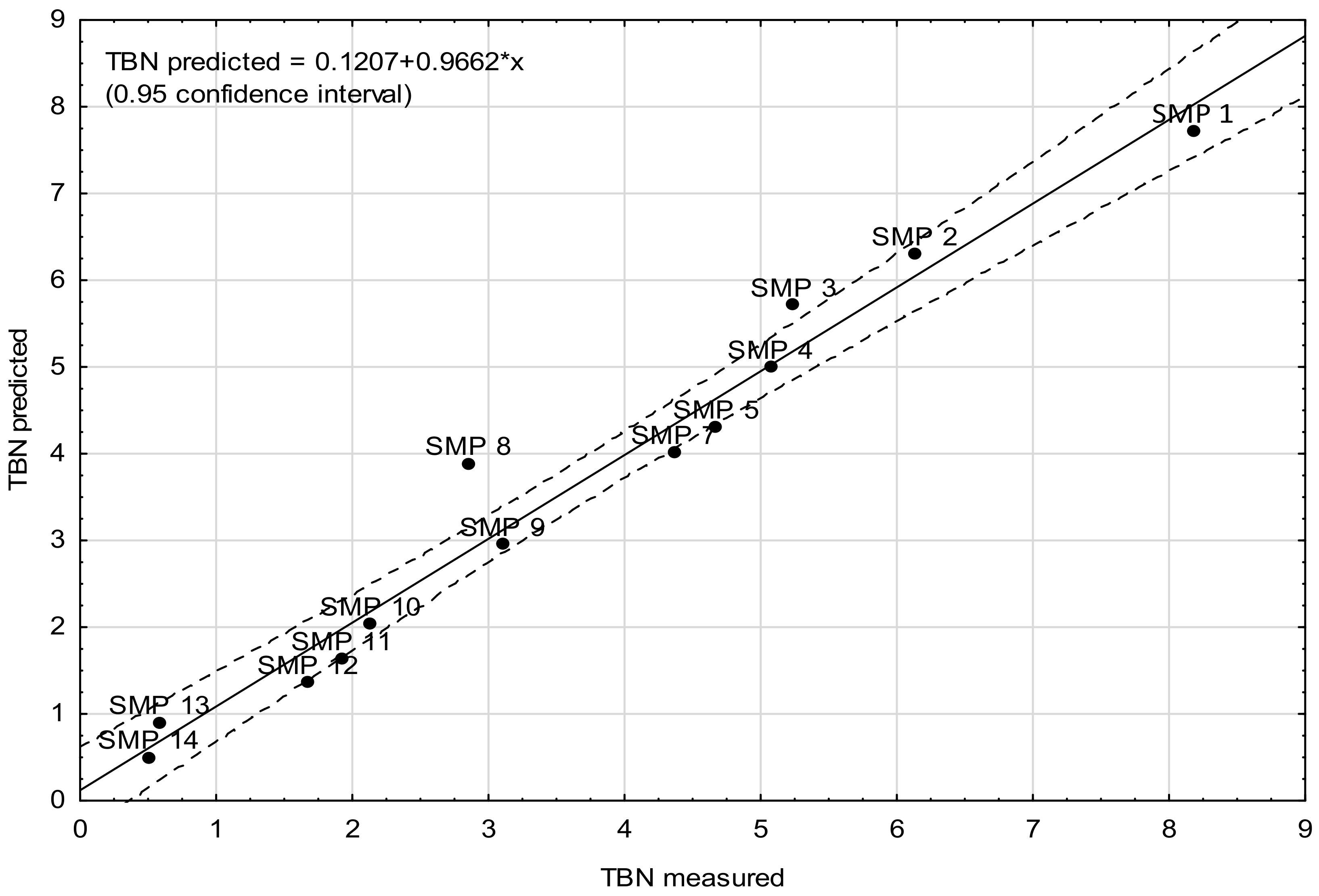
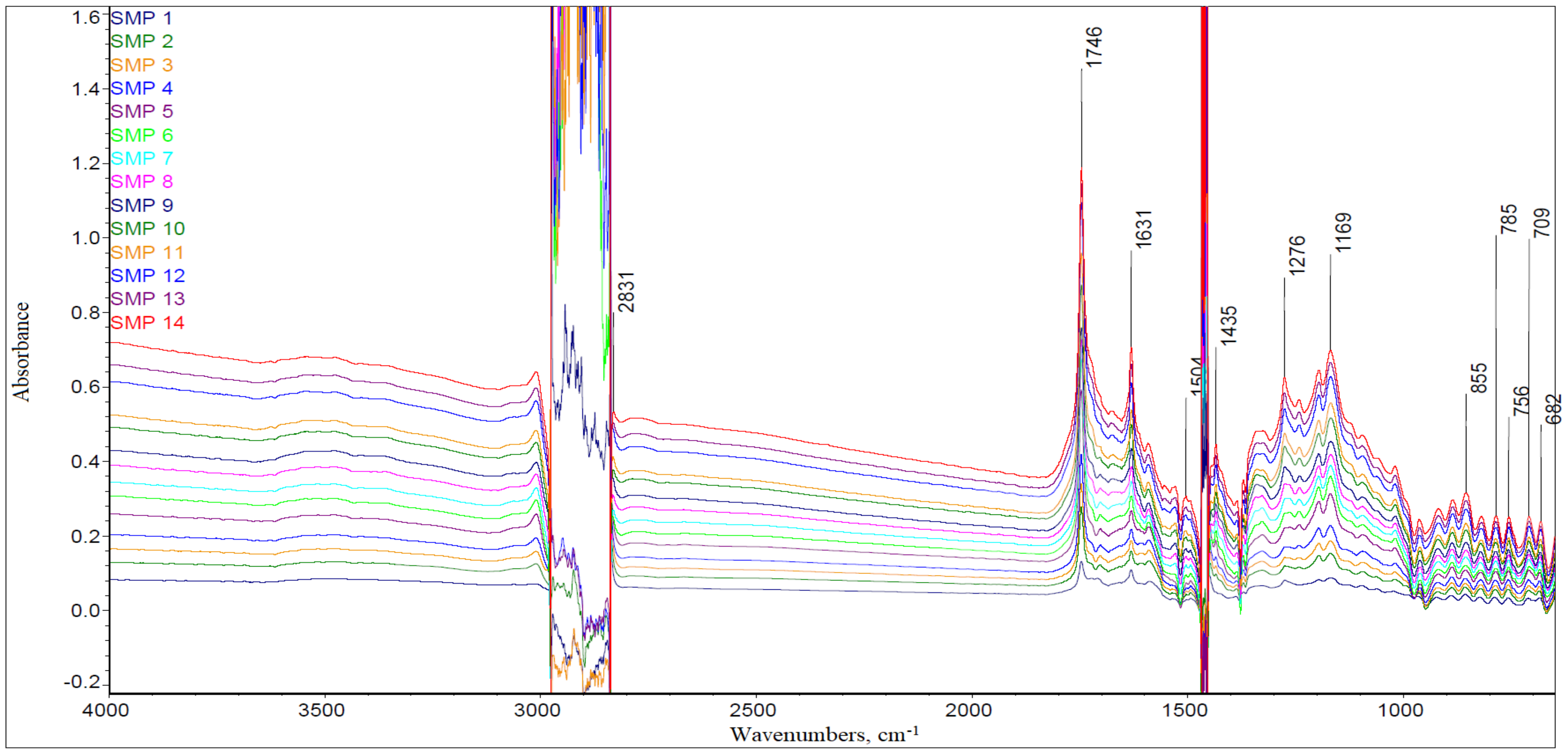
  • Model D—the model was based on the signal absorbance extremes at the wavenumbers corresponding to the molecular structures in chemical compounds that affect the base number value of the engine oil, i.e., 1746 cm−1 (carbonyls), 1631 cm−1 (nitro compounds), 1196 cm−1, 1169 cm−1, and 1062 cm−1 (sulfones and sulfonates).
  • Model E—the model was based on the measurement of the surface areas of selected spectral bands, formed in the spectra as a result of vibrations of molecular structures in chemical compounds, affecting the value of the base number of engine oil (similarly to Model D), i.e.,1746 cm−1 (carbonyls), 1631 cm−1 (nitro compounds), 1196 cm−1, 1169 cm−1, and 1062 cm−1 (sulfones and sulfonates).
In the case of Models D and E, it was assumed that the area below 1000 cm−1 (related to the vibrations of aromatic rings, substituents in these rings, or long hydrocarbon chains) carries very little information. These are chemical compounds that do not significantly affect the alkaline reserve and thus the TBN.
Model A was heavily inspired by the data analysis presented in Macian et al. [38], where the dimensionality of the pre-processed full spectra was reduced to four aggregates through averaging. Models B and C have two less and one more variable in comparison to Model A, respectively. These two models were primarily constructed to test the changes in the prediction accuracy with differing number of variables and spectra ranges. Finally, the Model D and E are more theory than the data-driven ones.
The results for the Model C, i.e., the model with the highest R2 and the smallest root mean square error (RMSE), out of all models tested, are shown in Table 4 and Table 5 and Figure 7. For each model, the first table presents the estimation results of the linear regression model and the model fit statistics (R2, adjusted R2, and RMSE), whereas the second table presents the raw input and output data used in modeling.
Table 3 shows the estimated linear Equation (1) for Model C in the following form:
TBN (prediction) = 9.682 + (ν <1000) × 316.270 + (ν 1000–1450) × (−10.326) + (ν 1475–1800) × (−133) + (ν 1800–2830) × (−36.081) + (ν 2975–4000) × 3.841
It makes the TBN prediction from the pre-processed FTIR measurements possible. Model C achieved very high R2 and adjusted R2 values, both well above the 90% threshold. What is more, the RMSE equal to 0.4050 is a satisfactory value. On average, the TBN predictions from Model C are by 0.4050 units different than the measured values of TBN. Figure 7 is a standard “observed vs. predicted” graph and shows the accuracy of Model C predictions.
Table 6 shows the estimated linear Equation (2) for Model D in the form of
TBN (prediction) = 9.033 + (ν 1746) × 38.416 + (ν 1631) × (14.971) + (ν 1196) × (−287.984) + (ν 1169) × 82.665+ (ν 1062) × 154.500
Model D (Table 6 and Table 7 and Figure 8) also achieved very high R2 and adjusted R2 values, but lower than for Model C. The RMSE equal to 0.4313 is also lower than for Model C, but it can be deemed a satisfactory value. On average, the TBN predictions from Model D are by 0.431 units different than the measured values of TBN. In a similar fashion, the regression equations for the remaining models can be obtained.
To reduce the information overload, the detailed results for Models A, B, and E are shown in Appendix A. Table 8 shows the results of R2, adjusted R2, and the RMSE for all developed models. By far the best model is Model C, and the worst results were obtained for Model B. When comparing Models D and E (the models based on the signal peak and the peak area), it should be highlighted that Model D, based on the signal (intensity peak, the one which exhibits the highest concentration), turned out to be slightly better than Model E, based on the peak area.
Analyzing Table 8 and Table 9, it can be observed that in terms of the mean percentage error, Model D seems to be the best one. For Model C, which turned out to be the best in terms of R2 and RMSE, the difficulties in predictions are caused by the samples from SMP 8 up to SMP 14, for which the largest percentage deviations between the measured and the predicted TBN were noticed. The division into high and low TBN values (SMP 1–7 and SMP 8–14) and the mean percentage errors for them confirm this observation. Nevertheless, the authors wish to point out that the compared measures (R2 and RMSE vs. average percentage error) are not compatible with each other. They can be considered as complementary rather than substitutive measures. The mean percentage error is particularly sensitive to low outliers (for Model C it was the sample SMP 13). In light of this, it seems that the final conclusions should be drawn on the basis of R2 and the RMSE only.

5. Discussions

An in-depth query of the existing literature revealed the paucity of similar research to the one undertaken in this study. Only three articles are to some degree connected to our research. Both of them were published very recently, underscoring the fact that this line of research is starting to gain traction in the literature.
Agocs and al. also investigated engine oil during its service life; however, they put a stress on a comprehensive tribological assessment [40]. They presented FT-IR results averaged from 32 transmission scans and TBN from two titrations and elemental composition; however, they did not compare those factors each other [40]. In their work, they demonstrated that TBN is between 6.5 mg KOH/g (sample 0 km) and 3.1 mg KOH/g (sample 20,000 km). The oxidation (FTIR) is 0.0 and 30.2, respectively. They also found the results for 5000 km, 8000 km, 9500 km and 13,500 km, which confirms that TBN gradually decreased during exploitation (6.0, 5.1, 4.8., and 3.7, respectively), whereas oxidation increased (7.5, 10.6, 12.3, and 19.1, respectively) [40]. This result confirms that the changes of TBN and FTIR parameters are similar for different oils (differently operated) and that it is reasonable to look for models describing changes in one parameter based on the data of the other.
Nagy and al. presented the PCA (Principal Component Analysis) method, which is a user-friendly approach to fleet tracking and oil condition monitoring in case of both condition-based and predictive maintenance strategies [33]. They also confirmed that based on a simple FT-IR spectra, no further oil analyses, e.g., NNand TBN titrations of water content evaluation, are required [33]. They indicated that the “loss of information” is minimal, as most conventional parameters are indirectly contained [33]. Contrary to our approach, they provided a methodology for rapid analysis for large vehicle fleets or sample sizes, using only Fourier-transformed infrared spectroscopy and the multivariate data analysis.
FTIR spectrometry in combination with partial least squares (PLS) and principal component regression (PCR) was also investigated by Sejkorova et al. [41], who proposed and tested as an alternative to the standardized method for determining the kinematic viscosity at 100 °C with an Ubbelohde capillary viscometer (CSN EN ISO 3104) of worn-out motor oil grade SAE 15W-40. The FTIR-PLS model in the spectral region of 1750–650 cm−1 with modification of the spectra by the second derivative proved to be the most suitable. A significant dependence of R = 0.95 was achieved between the viscosity values and the values predicted by the FTIR-PLS model. They concluded that the proposed method for determining the kinematic viscosity at 100 °C by the FTIR-PLS model is faster compared to the determination according to the CSN EN ISO 3104 standard, requires a smaller amount of oil sample for analysis, and produces less waste chemicals.

6. Conclusions

The analysis of the obtained FTIR spectra has led to the determination of the physicochemical foundations of building statistical models for the prediction of the TBN in engine oils, based on spectral measurements. The observed changes in the intensity of the bands in the spectra of oil illustrate the depletion of additives increasing the alkaline reserve (e.g., basic calcium sulfonate) and the formation of oil aging products. The substances, whose increase in oil content reduces the TBN, include, among others, the acidic products of thermal oxidation, nitration, and sulfonation. Thus, statistical models can be developed on the basis of the average absorbance values in the designated spectral ranges or on the basis of the measured intensity or surface area of specific spectral bands. All of the elaborated models are characterized by high R2, adjusted R2, and the RMSE values as well as acceptable levels of the average percentage error. Two of the built models are characterized by very high predictive capabilities (R2 > 0.98, RMSE < 0.5). These are Model C and Model D. Model C is based on average absorbance values calculated in five wavenumber ranges, i.e., <1000 cm−1, 1000–1450 cm−1, 1475–1800 cm−1, 1800–2830 cm−1, and 2975–4000 cm−1. In turn, Model D is based on the extreme values of the intensity of the bands at the wavenumbers corresponding to the molecular structures in the chemical compounds that affect the base number value of the engine oil. Additionally, Model D is characterized by the lowest mean percentage error. The developed statistical models may serve as a helpful tool for the quick TBN assessment of engine oils. Yet, their suitability for routine use in the diagnostics of the operational condition of engine oil requires further verification on a wider group of engine oils of different quality classes.

7. Limitations

It has to be underscored that the experiment consisted of a single run, which may to some degree limit the generalizability of the results. The future direction is to obtain a bigger data set to validate the models.

Author Contributions

Conceptualization, A.W., K.F. and J.M.; methodology, A.W., K.F. and J.M.; software, A.W., K.F. and J.M.; validation, A.W., K.F. and J.M.; formal analysis, A.W., K.F. and J.M.; investigation, A.W., K.F. and J.M.; resources, A.W., K.F. and J.M.; data curation, A.W., K.F. and J.M.; writing—original draft preparation, A.W., K.F., J.M. and B.Ł.; writing—review and editing, A.W., K.F. and J.M.; visualization, A.W. and K.F.; supervision, A.W., K.F. and J.M.; project administration, A.W.; funding acquisition, A.W., K.F. and J.M. All authors have read and agreed to the published version of the manuscript.

Funding

This research received no external funding.

Institutional Review Board Statement

Not applicable.

Informed Consent Statement

Not applicable.

Data Availability Statement

Not applicable.

Acknowledgments

This publication was financed with subsidies for maintaining the research capacity granted to the Cracow University of Economics. The work was financed also by the subvention Research Network Lukasiewicz—Institute for Sustainable Technologies in Radom.

Conflicts of Interest

The authors declare no conflict of interest.

Appendix A

Table A1. The results of the estimation of the TBN regression model (Model A).
Parameter Regression Coefficient
Intercept9.534
ν <1000233.191
ν 1000–2000−122.828
ν 2000–3000−156.564
ν >300097.462
Model fit statistics: R2 = 0.9728, adjusted R2 = 0.9592, and root mean square error = 0.4599.
Table A2. Average values for the defined spectral ranges and the TBN values (measured vs. predicted—Model A).
Sample Predictor ValueTBN
(Measured)
TBN
(Model Prediction)
ν <1000ν 1000–2000ν 2000–3000ν >3000
SMP 10.02810.05840.05530.07758.187.81
SMP 20.04170.09310.08380.12056.136.44
SMP 30.05080.11420.10650.15315.245.61
SMP 40.06290.13850.12980.18835.075.22
SMP 50.08240.17760.16480.23884.674.41
SMP 70.11000.23030.21750.31794.363.83
SMP 80.12270.25620.24690.36102.853.21
SMP 90.13610.28290.27430.40043.102.60
SMP 100.15870.32010.31220.45402.132.58
SMP 110.16880.34160.33260.48351.921.98
SMP 120.19820.39220.38910.56171.671.39
SMP 130.21380.42090.41850.60410.581.06
SMP 140.23020.45180.45500.65430.500.26
Table A3. The results of the estimation of the TBN regression model (Model B).
ParameterRegression Coefficient
Intercept8.074
ν 1000–1450−35.530
ν 1475–180017.638
Model fit statistics: R2 = 0.9496, adjusted R2 = 0.9396, and root mean square error = 0.5596.
Table A4. Average values for the defined spectral ranges and the TBN values (measured vs. predicted—Model B).
SamplePredictor ValueTBN
(Measured)
TBN
(Model Prediction)
ν 1000–1450 ν 1475–1800
SMP 10.05980.06278.187.06
SMP 20.09600.09966.136.42
SMP 30.11770.12105.246.03
SMP 40.14320.14505.075.54
SMP 50.18550.18294.674.71
SMP 70.24000.23774.363.74
SMP 80.26660.26482.853.27
SMP 90.29440.29323.102.78
SMP 100.32890.33632.132.32
SMP 110.34970.36181.922.03
SMP 120.39830.41761.671.29
SMP 130.42650.44890.580.84
SMP 140.45630.48250.500.37
Table A5. The results of the estimation of the TBN regression model (Model E).
Parameter Regression Coefficient
Intercept9.839
ν 17460.711
ν 1631−4.814
ν 1196−11.912
ν 11691.568
ν 1062−12.268
Model fit statistics: R2 = 0.9662, adjusted R2 = 0.9421, and root mean square error = 0.5480.
Table A6. Average values for the defined spectral ranges and the TBN values (measured vs. predicted—Model E).
Sample Predictor Value (Based on the Area Peak)TBN
(Measured)
TBN
(Model Prediction)
ν 1746ν 1631ν 1196ν 1169ν 1062
SMP 12.17800.53700.08300.26500.04108.187.73
SMP 23.72800.58800.29000.59800.06806.136.31
SMP 34.29600.60700.39900.70800.05005.245.72
SMP 45.24300.65900.53200.85200.03205.075.00
SMP 57.78700.88600.74101.42600.01704.674.31
SMP 79.94001.38200.72801.84300.03704.364.02
SMP 810.89301.68100.67601.94500.04902.853.89
SMP 912.02602.10600.66402.15900.06303.102.96
SMP 1014.59902.47500.74802.47600.10102.132.04
SMP 1116.66302.69700.81302.70900.13301.921.64
SMP 1219.85702.99100.90502.95200.16701.671.36
SMP 1321.43803.33400.90703.07400.17500.580.91
SMP 1422.45603.55200.91103.12500.18400.500.50
Figure A1. Measured vs. predicted value of TBN (Model A).
Energies 15 02809 g0a1
Figure A2. Measured vs. predicted value of TBN (Model B).
Energies 15 02809 g0a2
Figure A3. Measured vs. predicted value of TBN (Model E).
Energies 15 02809 g0a3

References

  1. Khaziev, A.; Laushkin, A. Investigation of Changes in the Properties of Engine Oil Depending on the Sulfur Content in Gasoline. IOP Conf. Ser. Mater. Sci. Eng. 2020, 832, 012080. [Google Scholar] [CrossRef]
  2. Patel, N.; Shadangi, K.P. Characterization of Waste Engine Oil (WEO) Pyrolytic Oil and Diesel Blended Oil: Fuel Properties and Compositional Analysis. Mater. Today Proc. 2020, 33, 4933–4936. [Google Scholar] [CrossRef]
  3. Tayari, S.; Abedi, R.; Rahi, A. Comparative Assessment of Engine Performance and Emissions Fueled with Three Different Biodiesel Generations. Renew. Energy 2020, 147, 1058–1069. [Google Scholar] [CrossRef]
  4. Tayari, S.; Abedi, R.; Tahvildari, K. Experimental Investigation on Fuel Properties and Engine Characteristics of Biodiesel Produced from Eruca Sativa. SN Appl. Sci. 2020, 2, 2. [Google Scholar] [CrossRef] [Green Version]
  5. ASTM D8045-17e1; Standard Test Method for Acid Number of Crude Oils and Petroleum Products by Catalytic Thermometric Titration. ASTM International: West Conshohocken, PA, USA, 2017. [CrossRef]
  6. ASTM D974-14e2; Standard Test Method for Acid and Base Number by Color- Indicator Titration. ASTM International: West Conshohocken, PA, USA, 2014. [CrossRef]
  7. ASTM D664-18e2; Standard Test Method for Acid Number of Petroleum Products by Potentiometric Titration. ASTM International: West Conshohocken, PA, USA, 2018. [CrossRef]
  8. Wanke, P. In-Use Investigations of the Changes of Lubricant Properties in Diesel Engines. TEKA Comm. Mot. Energ. Agric. 2012, 12, 263–267. [Google Scholar]
  9. Masuko, M.; Ohkido, T.; Suzuki, A.; Ueno, T.; Okuda, S.; Sagawa, T. Fundamental Study of Changes in Friction and Wear Characteristics Due to ZnDTP Deterioration in Simulating Engine Oil Degradation during Use (Part 2)—Influences of the Presence of Peroxide and Dispersed Zn-Containing Solids. Dirac’s Differ. Equ. Phys. Finite Differ. 2005, 48, 769–777. [Google Scholar] [CrossRef]
  10. Vasanthan, B.; Devaradjane, G.; Shanmugam, V. Online Condition Monitoring of Lubricating Oil on Test Bench Diesel Engine & Vehicle. J. Chem. Pharm. Sci. 2015, 2015, 315–320. [Google Scholar]
  11. Kral, J.; Konecny, B.; Madac, K.; Fedorko, G.; Molnar, V. Degradation and Chemical Change of Longlife Oils Following Intensive Use in Automobile Engines. Measurement 2014, 50, 34–42. [Google Scholar] [CrossRef]
  12. Sharma, G.K.; Chawla, O.P. Modelling of Lubricant Oil Alkalinity in Diesel Engines. Tribol. Int. 1988, 21, 269–274. [Google Scholar] [CrossRef]
  13. Wolak, A. TBN Performance Study on a Test Fleet in Real-World Driving Conditions Using Present-Day Engine Oils. Measurement 2018, 114, 322–331. [Google Scholar] [CrossRef]
  14. Sentanuhady, J.; Majid, A.I.; Prashida, W.; Saputro, W.; Gunawan, N.P.; Raditya, T.Y.; Muflikhun, M.A. Analysis of the Effect of Biodiesel B20 and B100 on the Degradation of Viscosity and Total Base Number of Lubricating Oil in Diesel Engines with Long-Term Operation Using ASTM D2896 and ASTM D445-06 Methods. TEKNIK 2020, 41, 269–274. [Google Scholar] [CrossRef]
  15. Chikunova, A.S.; Vershinin, V.I. Determination of the Total Base Number of Engine Oils Using Potentiometric Titration. Ind. Lab. Diagn. Mater. 2020, 86, 5–12. [Google Scholar] [CrossRef]
  16. Growney, D.; Trickett, K.; Robin, M.; Rogers, S.; McDowall, D.; Moscrop, E. Acid Neutralization Rates—Why Total Base Number Doesn’t Tell the Whole Story: Understanding the Neutralization of Organic Acid in Engine Oils. SAE Int. J. Fuels Lubr. 2021, 14, 297. [Google Scholar] [CrossRef]
  17. Nagy, A.L.; Knaup, J.C.; Zsoldos, I. Investigation of Used Engine Oil Lubricating Performance Through Oil Analysis and Friction and Wear Measurements. Acta Tech. Jaurinensis 2019, 12, 237–251. [Google Scholar] [CrossRef] [Green Version]
  18. Wei, L.; Duan, H.; Jin, Y.; Jia, D.; Cheng, B.; Liu, J.; Li, J. Motor Oil Degradation during Urban Cycle Road Tests. Friction 2021, 9, 1002–1011. [Google Scholar] [CrossRef]
  19. Agocs, A.; Budnyk, S.; Frauscher, M.; Ronai, B.; Besser, C.; Dörr, N. Comparing Oil Condition in Diesel and Gasoline Engines. Ind. Lubr. Tribol. 2020, 72, 1033–1039. [Google Scholar] [CrossRef]
  20. Besser, C.; Agocs, A.; Ronai, B.; Ristic, A.; Repka, M.; Jankes, E.; McAleese, C.; Dörr, N. Generation of Engine Oils with Defined Degree of Degradation by Means of a Large Scale Artificial Alteration Method. Tribol. Int. 2019, 132, 39–49. [Google Scholar] [CrossRef]
  21. Kurre, S.K.; Pandey, S.; Khatri, N.; Bhurat, S.S.; Kumawat, S.K.; Saxena, S.; Kumar, S. Study of Lubricating Oil Degradation of Ci Engine Fueled with Diesel-Ethanol Blend. Tribol. Ind. 2021, 43, 222. [Google Scholar] [CrossRef]
  22. Robinson, N.; Hons, B.S. Monitoring Oil Degradation with Infrared Spectroscopy. Set Point Technol. 2000, 5, 1–8. [Google Scholar]
  23. Dyson, B.A.; Richards, L.J.; Eng, B.S.; Sc, W.; Williams, K.R.; Sc, B. Diesel Engine Lubricants: Their Selection and Utilization with Particular Reference to Oil Alkalinity. Ind. Lubr. Tribol. 1988, 9, 34–40. [Google Scholar] [CrossRef]
  24. Kauffman, R.E. Rapid, Portable Voltammetric Techniques for Performing Antioxidant, Total Acid Number (TAN) and Total Base Number (TBN) Measurements. Lubr. Eng. 1998, 54, 39–46. [Google Scholar]
  25. Bassbasi, M.; Hafid, A.; Platikanov, S.; Tauler, R.; Oussama, A. Study of Motor Oil Adulteration by Infrared Spectroscopy and Chemometrics Methods. Fuel 2013, 104, 798–804. [Google Scholar] [CrossRef]
  26. Agoston, A.; Schneidhofer, C.; Dörr, N.; Jakoby, B. A Concept of an Infrared Sensor System for Oil Condition Monitoring. Elektrotechnik Inf. 2008, 125, 71–75. [Google Scholar] [CrossRef]
  27. Barra, I.; Kharbach, M.; Qannari, E.M.; Hanafi, M.; Cherrah, Y.; Bouklouze, A. Predicting Cetane Number in Diesel Fuels Using FTIR Spectroscopy and PLS Regression. Vib. Spectrosc. 2020, 111, 103157. [Google Scholar] [CrossRef]
  28. Liu, Y.; Bao, K.; Wang, Q.; Zio, E. Application of FTIR Method to Monitor the Service Condition of Used Diesel Engine Lubricant Oil. In Proceedings of the 2019 4th International Conference on System Reliability and Safety, ICSRS 2019, Rome, Italy, 20–22 November 2019. [Google Scholar]
  29. Gracia, N.; Thomas, S.; Bazin, P.; Duponchel, L.; Thibault-Starzyk, F.; Lerasle, O. Combination of Mid-Infrared Spectroscopy and Chemometric Factorization Tools to Study the Oxidation of Lubricating Base Oils. Recent Dev. Operando Spectrosc. 2010, 155, 255–260. [Google Scholar] [CrossRef]
  30. Adams, M.J.; Romeo, M.J.; Rawson, P. FTIR Analysis and Monitoring of Synthetic Aviation Engine Oils. Talanta 2007, 73, 629–634. [Google Scholar] [CrossRef]
  31. Holland, T.; Abdul-Munaim, A.M.; Mandrell, C.; Karunanithy, R.; Watson, D.G.; Sivakumar, P. Uv-Visible Spectrophotometer for Distinguishing Oxidation Time of Engine Oil. Lubricants 2021, 9, 37. [Google Scholar] [CrossRef]
  32. Chimeno-Trinchet, C.; Murru, C.; Díaz-García, M.E.; Fernández-González, A.; Badía-Laíño, R. Artificial Intelligence and Fourier-Transform Infrared Spectroscopy for Evaluating Water-Mediated Degradation of Lubricant Oils. Talanta 2020, 219, 121312. [Google Scholar] [CrossRef]
  33. Nagy, A.L.; Agocs, A.; Ronai, B.; Raffai, P.; Rohde-Brandenburger, J.; Besser, C.; Dörr, N. Rapid Fleet Condition Analysis through Correlating Basic Vehicle Tracking Data with Engine Oil FT-IR Spectra. Lubricants 2021, 9, 114. [Google Scholar] [CrossRef]
  34. Wilson, D.; Allen, C. Experimental Validation of an Unscented Kalman Filter for Estimating Transient Engine Exhaust Composition with Fourier Transform Infrared Spectroscopy. Energy Fuels 2018, 32, 11899–11912. [Google Scholar] [CrossRef]
  35. Taghizadeh, A.; D’Souza, M. Quantification of Active Antioxidants by FTIR Spectroscopy and the Correlation to Measured TBN Values. SAE Tech. Pap. 2001, 110, 2072–2077. [Google Scholar] [CrossRef]
  36. Dong, J.; van de Voort, F.R.; Yaylayan, V.; Ismail, A.A.; Pinchuk, D.; Taghizadeh, A. Determination of Total Base Number (TBN) in Lubricating Oils by Mid-FTIR Spectroscopy. Lubr. Eng. 2001, 57, 24–30. [Google Scholar]
  37. Sejkorová, M.; Šarkan, B.; Veselík, P.; Hurtová, I. FTIR Spectrometry with PLS Regression for Rapid TBN Determination of Worn Mineral Engine Oils. Energies 2020, 13, 6438. [Google Scholar] [CrossRef]
  38. Macián, V.; Tormos, B.; García-Barberá, A.; Tsolakis, A. Applying Chemometric Procedures for Correlation the FTIR Spectroscopy with the New Thermometric Evaluation of Total Acid Number and Total Basic Number in Engine Oils. Chemom. Intell. Lab. Syst. 2021, 208, 104215. [Google Scholar] [CrossRef]
  39. R Core Team. R: A Language and Environment for Statistical Computing; R Foundation for Statistical Computing: Vienna, Austria, 2019; Available online: https://www.r-project.org/ (accessed on 1 March 2021).
  40. Agocs, A.; Besser, C.; Brenner, J.; Budnyk, S.; Frauscher, M.; Dörr, N. Engine Oils in the Field: A Comprehensive Tribological Assessment of Engine Oil Degradation in a Passenger Car. Tribol. Lett. 2022, 70, 28. [Google Scholar] [CrossRef]
  41. Sejkorová, M.; Kučera, M.; Hurtová, I.; Voltr, O. Application of FTIR-ATR Spectrometry in Conjunction with Multivariate Regression Methods for Viscosity Prediction of Worn-out Motor Oils. Appl. Sci. 2021, 11, 3842. [Google Scholar] [CrossRef]
Figure 1. The FTIR differential spectra for the samples of the regions 650–4000 cm−1.
Energies 15 02809 g001
Figure 2. The FTIR differential spectra for the samples of the regions 1475–1800 cm−1.
Energies 15 02809 g002
Figure 3. The intensity of the band at the wavenumber of 1746 cm−1 in the recorded spectra of the engine oil samples tested.
Energies 15 02809 g003
Figure 4. The FTIR differential spectra for the samples, the regions 1000–1450 cm−1.
Energies 15 02809 g004
Figure 5. Changes in the TBN of engine oils.
Energies 15 02809 g005
Figure 6. The chemical structure of an exemplary enriching additive of TBN.
Energies 15 02809 g006
Figure 7. Measured vs. predicted value of TBN (Model C).
Energies 15 02809 g007
Figure 8. Measured vs. predicted value of TBN (Model D).
Energies 15 02809 g008
Table 1. The general specification of the selected car.
The ParameterThe Value
Maximum torque340 Nm at 2000 rpm
Forced inductionTurbocharger (gas compressor)
Number of cylinders4
Cylinder arrangementStraight (inline)
Number of valves16
Injection typeCommon Rail
Lubrication system capacity5.5 L
Manual gearbox6-gear
Transmission typeRear axle
Table 2. Operational characteristics of the tested vehicle.
Sample CodeNumber of In-Service DaysSampling Date
(D-M-Y)
Mileage [km]
SMP 0017.7.20190
SMP 1017.7.201913
SMP 22815.8.20191157
SMP 34229.8.20192175
SMP 45512.9.20193116
SMP 51052.11.20194220
SMP 615017.12.20195265
SMP 71707.1.20206332
SMP 820815.2.20207319
SMP 92907.5.20208498
SMP 1033219.6.20209811
SMP 1135411.7.202011,021
SMP 124096.9.202012,460
SMP 134363.10.202013,521
SMP 144707.11.202014,820
Table 3. Percentage changes in the TBN in relation to the changes in the intensity of the selected spectral bands (FTIR) of the tested samples.
Sample CodeTBNA at 1746 cm−1A at 1631 cm−1A at 1169 cm−1
SMP 1 *8.18 mg KOH/g0.1310.1090.087
Relative Change
SMP 2−25%111%46%76%
SMP 3−15%23%18%22%
SMP 4−3%23%17%22%
SMP 5−8%42%23%38%
SMP 7−7%4%13%8%
SMP 8−35%4%11%8%
SMP 99%4%12%9%
SMP 10−31%15%15%14%
SMP 11−10%10%8%8%
SMP 12−13%14%13%13%
SMP 13−65%5%8%6%
SMP 14−14%4%7%5%
* A reference sample.
Table 4. The results of the estimation of the TBN regression model (Model C).
ParameterRegression Coefficient
Intercept9.682
ν <1000316.270
ν 1000–1450−10.326
ν 1475–1800−133.000
ν 1800–2830−36.081
ν 2975–40003.841
Model fit statistics: R2 = 0.9815, adjusted R2 = 0.9684, and root mean square error = 0.4050.
Table 5. Average values for defined spectral ranges and the TBN (measured vs. predictions for Model C).
Sample Predictor ValueTBN
(Measured)
TBN
(Model Prediction)
ν <1000ν 1000–1450ν 1475–1800ν 1800–2830ν 2975–4000
SMP 10.02810.05980.06270.05240.07718.188.03
SMP 20.04170.09600.09960.08000.11966.136.20
SMP 30.05080.11770.12100.10100.15245.245.40
SMP 40.06290.14320.14500.12430.18705.075.04
SMP 50.08240.18550.18290.15820.23714.674.69
SMP 70.11000.24000.23770.21020.31524.364.00
SMP 80.12270.26660.26480.23770.35832.853.33
SMP 90.13610.29440.29320.26290.39793.102.74
SMP 100.15870.32890.33630.30070.45072.132.63
SMP 110.16880.34970.36180.31960.48041.921.66
SMP 120.19820.39830.41760.37360.55831.671.37
SMP 130.21380.42650.44890.40220.60040.580.99
SMP 140.23020.45630.48250.43750.65030.500.32
Table 6. The results of the estimation of the TBN regression model (Model D).
Parameter Regression Coefficient
Intercept9.033
ν 174638.416
ν 163114.971
ν 1196−287.984
ν 116982.665
ν 1062154.500
Model fit statistics: R2 = 0.9791, adjusted R2 = 0.9641, and root mean square error = 0.4313.
Table 7. Average values for the defined spectral ranges and the TBN values (measured vs. predicted, Model D).
Sample Predictor Value (Based on the Signal Peak) TBN
(Measured)
TBN
(Model Prediction)
ν 1746ν 1631ν 1196ν 1169ν 1062
SMP 10.13140.10900.08300.08690.05758.187.87
SMP 20.27660.15890.14660.15320.09026.136.41
SMP 30.34000.18710.18010.18630.11145.245.64
SMP 40.41830.21800.22060.22690.13675.074.72
SMP 50.59220.26800.29240.31350.17484.674.51
SMP 70.70190.34610.35950.38830.22314.364.23
SMP 80.72740.38590.38770.41800.24482.853.49
SMP 90.75880.43380.41930.45370.26723.102.70
SMP 100.87300.49810.47450.51630.29942.132.32
SMP 110.95910.53810.50990.55660.31621.921.95
SMP 121.09480.60980.57740.62750.35901.671.28
SMP 131.14520.66050.61200.66520.38290.580.80
SMP 141.18730.70540.64400.69680.40870.500.48
Table 8. The comparison of the parameter values of R2, adjusted R2, and the RMSE for Models A, B, C, D, and E.
Model Fit StatisticsModel AModel BModel CModel D Model E
R20.9730.9500.9820.9800.966
Adjusted R20.9590.9400.9680.9640.942
Root mean square error0.4600.5600.4050.4310.548
Table 9. The comparison of the results (mean percentage error) for Models A, B, C, D, and E.
Model AModel BModel CModel DModel E
1 *2 *1 *2 *1 *2 *1 *2 *1 *2 *
SMP 10.375%1.1214%0.152%0.314%0.456%
SMP 20.315%0.295%0.071%0.285%0.183%
SMP 30.377%0.7915%0.163%0.408%0.489%
SMP 40.153%0.479%0.031%0.357%0.071%
SMP 50.266%0.041%0.021%0.163%0.368%
SMP 70.5312%0.6214%0.368%0.133%0.348%
SMP 80.3613%0.4215%0.4817%0.6422%1.0437%
SMP 90.5016%0.3210%0.3612%0.4013%0.145%
SMP 100.4521%0.199%0.5023%0.199%0.094%
SMP 110.063%0.116%0.2613%0.032%0.2815%
SMP 120.2817%0.3823%0.3018%0.3923%0.3118%
SMP 130.4882%0.2644%0.4172%0.2238%0.3357%
SMP 140.2449%0.1326%0.1836%0.024%0.001%
mean0.3418%0.4015%0.2516%0.2711%0.3113%
SMP 1–70.336%0.3310%0.263%0.275%0.306%
SMP 8–140.3329%0.3419%0.2827%0.2716%0.3119%
1 *—the absolute value of the difference in the TBN between the measured and the predicted value [mg KOH/g]. 2 *—the percentage difference between the measured and the predicted value [%].
Publisher’s Note: MDPI stays neutral with regard to jurisdictional claims in published maps and institutional affiliations.

