Abstract
Maintenance plays a crucial role in the availability of an asset. In particular, when a company’s assets are decentralized, logistical aspects directly impact maintenance management and, consequently, productivity. In the energy generation sector, this scenario is common in enterprises and projects in which distributed energy resources (DERs), such as small hydroelectric power plants (SHPPs), are considered. Hence, the objective of this work is to propose an application of generalized stochastic Petri nets (GSPN) for the planning and optimization of the maintenance logistics of a DER enterprise with two SHPPs. In the presented case study, different scenarios are modeled considering logistical aspects related to the availability of spare parts and the sharing of maintenance teams between plants. From the financial return resulting from the estimated energy generation and the operating cost of each simulated scenario, the most profitable one can be estimated. The results demonstrate the ability of GSPNs to estimate the influence of the number of spare parts and maintenance teams on the availability of DERs, allowing the optimization of costs related to maintenance logistics.
1. Introduction
The global demand for energy, even in the face of economic, financial, and health crises, continues to grow exponentially [1,2], requiring the optimization of existing generating systems and the implementation of new projects and endeavors. At the same time, given the need to reduce greenhouse gas emissions, the generation of electricity from clean and renewable energy sources has been intensified, while the use of fossil fuels has been reduced.
In this scenario, the generation of electricity considering hydroelectric power plants (HPP) becomes very attractive for several reasons, but principally because these are a more stable source than other clean energy sources such as solar and wind power. In particular, small hydroelectric power plants (SHPPs) have been standing out all over the world, mainly due to their short construction period, easy maintenance, high energy density, and local distributed energy generation capacity [3,4,5].
Notably, being a distributed energy resource (DER), SHPPs have been widely implemented by underdeveloped and developing nations in the last years, enabling a large part of the population, especially in rural areas, to have access to electricity [5]. Many of these countries, such as Brazil, adopt an open market business environment for electricity generation, in which both private and public companies can freely negotiate the electricity supply, following the regulations of the sector.
In this trading environment, investments not only in SHPPs but also in renewable energy generation as a whole, bring benefits from a socio-environmental point of view, in addition to being financially advantageous, as presented by a survey released by Imperial College London and the International Energy Agency [6]. Taking as an example some countries in Europe and the United States, investments in renewable energy in Germany and France generated returns of around 178% between 2015 and 2020, compared to a negative return of around 21% for investments in fossil fuels. In the UK, meanwhile, over the same period, investments in green energy generated returns greater than 75% compared to less than 9% for fossil fuels. In the US, renewable energies yielded more than 200% of return against practically half of this value for fossil fuels.
However, as attractive as these investments can be, no business can thrive without good planning and proper management. Among other aspects that demand the attention of administrators and managers is the availability of energy generation equipment, which is directly influenced by its reliability and maintainability. Would maximizing equipment availability, and consequently energy production, be the best approach in these cases to maximize the financial return?
Despite the opportunities and demand from customers, the constant pressure to reduce operating costs imposed on aggregators, mainly due to fierce competition, has increasingly highlighted the importance of effective maintenance and associated logistics. In other words, the cost considerations involved in getting the necessary human and material resources in the right place in the shortest possible time have become a critical issue for maintenance planners and managers at any stage of the life cycle of an enterprise. In the authors’ experience, cost reduction in the case of DERs herein contemplates two critical considerations: keeping spare parts inventories to a minimum and sharing the maintenance workforce between sites. The former consideration prevents immobilization of otherwise much-needed capital and eliminates the need for costly and burdensome preservation of shelf items. The latter provides a more effective allocation of the available human resources.
In the quest to find a balance between costs and the conservation of equipment performance, new methodologies are adopted and applied to improve the efficiency, quality, and reliability of the repairable systems [7]. Some works that seek to develop more realistic techniques using simulation models to analyze the reliability and availability of systems are already found in the literature. Such models are very useful in the case of complex systems and propose, based on the understanding of the analyzed system, the application of generalized stochastic Petri nets (GSPN) [7,8,9,10].
Continuing in this line of research, the present work proposes an application of GSPNs in which a DER enterprise with two SHPPs is modeled, taking into account logistical aspects related to the availability of spare parts and the sharing of maintenance teams between units. The method proposed for the development of this application is based on the study of the considered systems, the collection of data related to failures and repairs of these systems’ components, and the estimation of time for the displacement of maintenance teams between the systems’ sites and for the purchase and arrival of spare parts to these sites.
Different GSPN models are considered where the number of available maintenance teams and the availability of spare parts varies. From the financial return resulting from the estimated energy generation and the operating cost of each case, the most profitable scenario can be estimated. The chosen approach mainly aims to demonstrate the applicability of GSPNs as a modeling tool to optimize and plan the most efficient maintenance logistics of DERs projects. The results obtained in this article demonstrate the capacity and potential use of GSPN for this task, in addition to its already well-known ability to estimate the availability and reliability of engineering systems.
2. Generalized Stochastic Petri Net
Petri net (PN) was first documented by Carl Adam Petri back in 1962 as part of his Ph.D. dissertation, Kommunikation mit Automaten (Communication with Automaton), describing the casual relationships between conditions and events in computer systems [7,8,9,10,11], although some claim that this technique was originally invented by Petri in 1939 at the age of 13 to model chemical processes. However, the current graphical representation of PNs emerged in the mid-1960s [12].
This combination of graphical, mathematical, and simulation techniques for modeling, interpretation, visualization, and optimization of complex systems with concurrent, distributed, stochastic (or non-deterministic), and both continuous and discrete features, have been used in a wide range of domains, directly benefiting from the theoretical foundations developed in the last five decades [12,13,14].
Functionally, PNs resemble a flowchart or block diagram, being graphically represented by four fundamental elements: places (described by a circle that represents the state or condition of an object, component, or system), transitions (described by rectangles, boxes, or bars that allow the system state change, modeling its dynamic behavior), arcs (described by solid arrows that connect places to transitions and vice versa), and tokens (described by a black dot or small solid circle stored in places representing the state of the object, component, or system) [7,14,15].
In its original design, PNs did not contemplate the concept of time, and its transitions only enabled instantaneous changes in the states of the modeled system. However, in the late 1970s and early 1980s, the idea of a PN with “timed” transitions arose based on the dissertations of S. Natkin, published in 1980 at the Conservatoire National des Arts et Métiers in Paris, France, and of M. K. Molloy, published in 1981 at the University of California in Los Angeles, USA. These works were developed independently and virtually simultaneously, which led to the definition of almost identical models also named in the same way: stochastic Petri nets (SPN) [16].
An extension of SPNs in which two different classes of transitions are supported—immediate transitions (that describe logical behaviors), represented by solid bars, and timed transitions (that describe time-consuming activities’ execution), represented by open bars—are the generalized stochastic Petri nets (GSPNs) [15,17].
The GSPNs are defined through a six-element enuple, given by GSPN = (P, T, F, W, M0, Λ) [9,15,18], where:
- is a finite set of places;
- is a finite set of transitions;
- is a set of arcs;
- is a weight function;
- is the initial marking;
- is the set of firing rates associated with the transitions;
- and .
GSPN has been used in several application areas [12,15,19,20,21,22], including fault diagnosis [23,24,25] and reliability and availability analysis [7,26]. However, maintenance planning and optimization can be considered one of the most prominent fields of application of GSPN, given the applicability of this technique in modeling and analyzing systems composed of components and equipment with different failure and repair times. The way the system and the context in which it is inserted are modeled is fundamental in these cases, and different approaches are found in the literature.
Chang and Hsiang [26], e.g., apply GSPNs to decide the optimal maintenance policy and build models for different levels of maintenance and renewal for automated manufacturing systems with a serial-parallel layout. Basically, two models were built, the first one considered different levels of preventive maintenance, and in the second, different levels of renewal maintenance. The models adopted in these cases are composed of a large complex mesh that can be understood as a combination of four smaller PN, with several places and transitions.
Santos, Teixeira and Soares [27] apply GSPNs with predicates coupled with Monte Carlo simulation to model Operation and Maintenance (O&M) activities planning of an offshore wind turbine. Included in the modeling are three maintenance categories classified according to the dimensions and weight of the components to be replaced, and the logistics involved, considering the need for vessels, the availability of maintenance personnel and spare parts, as well as delays and associated costs. The meteorological conditions that define access windows to the wind turbines were also considered and modeled with PN. Two maintenance models (corrective and preventive with imperfect repair) were compared considering system availability, component failure rate, and O&M costs. In the following year of this article, the same authors presented an extension of their work in which different maintenance models were simulated and compared [10].
Melani et al. [9] use GSPNs to determine the effect that the number of maintenance teams has on the availability and performance of a coal-fired power plant cooling tower. Each cooling tower cell was modeled as a PN with five places (stable operation, operation with degradation, failure, equipment in predictive maintenance, and equipment in corrective maintenance) and several transitions, allowing the action of the available maintenance teams to occur before or after each equipment fails, causing several different scenarios to be considered. In addition, three models with one, two, and three maintenance teams, respectively, were considered and compared concerning plant availability, reliability, and efficiency.
Bateliƈ, Gripariƈ and Matika [28] apply GSPNs in modeling the operation of coal mills belonging to a thermoelectric power plant. The objective of the model was to evaluate the hypothesis that a maintenance strategy based on remediation would increase the effectiveness of the entire analyzed system. The model was described by three PN, two of which were designated as mill subsystems (the falling pipe and the coal feeder), considering three states (operational equipment, malfunctioning equipment, and failing equipment) where stochastic transition values are calculated based on probabilistic density distributions, and one designated the operation of the plant as a whole, in which two states are considered (plant operating and plant failing).
Elusakin et al. [14] present an SPN model for O&M planning of floating offshore wind turbines, including their supporting structure components. The proposed model incorporates all the interrelationships between the different factors that influence the O&M planning of these systems, including the deterioration and renewal process of its components. In addition to the system degradation process, the condition monitoring and maintenance process are modeled, each with a specific PN that makes up a single, more complex GSPN.
The GSPN’s ability to help estimate the availability and reliability of assets and systems are explored in the current work in a modular way, making the model capable of representing the logistical challenges associated with inventory management and maintenance team management. The next session will present the article’s proposed method.
3. Proposed Method
Figure 1 presents the step-by-step procedure proposed in the current work for the development of the GSPN model, which in turn will be used for estimating the influence of the number of spare parts and maintenance teams on the availability of the considered systems, thus allowing the optimization of costs related to maintenance and, consequently, maximizing the enterprise’s profit.
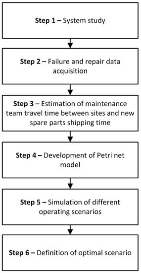
Figure 1.
The proposed method.
The first step of the proposed method is the study of the system. At this early stage, the assets to be represented in the PN need to be defined. It is also necessary to know the location of the assets, i.e., to which plant do they belong since the method was developed with DERs in mind. In this case, the use of a functional tree, which presents such components structurally and hierarchically, is recommended.
Once the assets to be represented in the GSPN are known, it is necessary to collect, for each of them, failure and repair data. Such data generally consist of time-to-failure and time-to-repair records for each component and can be acquired from the asset management system used by the company. This data is used so that the GSPN can emulate asset failures, implying maintenance actions. With these data in hand, it is possible to use the maximum likelihood estimation (MLE) to determine the probability distribution that better represents the probability of failure or repair at a given instant of time for each asset [9]. Alternatively, if such data are not properly recorded by the company, comprehensive reliability commercial databases can be used to obtain probability distributions.
In the third step, two new types of information need to be collected: the travel time that a maintenance team, based in the company’s headquarters, take to reach each of the plants to repair an eventually failed asset; and the time it takes for each spare part, once ordered, to be delivered by its manufacturer. Such data, if available, may also be collected through the company’s asset management system. Otherwise, the former can be estimated from the analysis of the distance to be traveled and the type and availability of roads between the company’s headquarters and the generating plants; and the latter can be obtained by consultation with spare parts manufacturers.
After collecting all the information previously described, it is possible, in the fourth step, to develop a GSPN that will emulate the behavior of the system under study. The GSPN proposed here can be divided into three main structures: the representation of the states of a component; the representation of the states of a spare part; and the representation of the maintenance teams states. Figure 2 shows in detail these three structures, where the black dots represent the tokens, circles represent places, white rectangles represent timing transitions, and black rectangles are direct transitions.
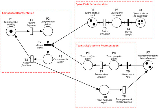
Figure 2.
The Generalized Stochastic Petri Nets (GSPN) proposed structures.
Still considering Figure 2, it can be seen that the asset is represented by three places (P1, P2, and P3) and three transitions (T1, T2, and T3). In the model, therefore, the asset can be in one of three possible conditions: in operation or working (P1), in failure (P2), or repair (P3). The current condition is informed by the position of the token that moves between such places through transition firings. For example, if the asset fails and ceases to perform its function (firing of transition T1), the token moves from P1 to P2. It is important to note that the firings of T1 and T3 are governed by the probabilistic distributions obtained in step 2 of the proposed method, i.e., they are timing transitions. T2 is a direct transition, which occurs immediately as soon as the conditions for such are satisfied (P2, P6, and P7 must have at least one token each for T3 to be fired, i.e., the component must be at fault, it must have a spare part in stock, and the maintenance team needs to be at the plant).
The representation of spare parts management in the model is done through three places (P4, P5, and P6) and two transitions (T5 and T6). Place P4 represents the existence of spare parts to be purchased from suppliers, so it must have a large number of tokens, at least enough so that P4 is never empty during the time interval considered during the GSPN simulation. A token goes from P4 to P5 if a purchase of a spare part is necessary, that is, T4 is fired only when the number of tokens (spare parts) in P6 (in stock) is less than planned or when a component failure occurs. T5, on the other hand, is triggered only when the purchased part arrives in stock and, as there is a time delay between purchase and delivery, T5 is also a timing transition, governed by the information collected in step 3 of the method.
The representation of the maintenance team’s work is done through four places (P7, P8, P9, and P10) and three transitions (T6, T7, and T8). The tokens in P7 represent the number of maintenance teams available to attend to one or more failures that may occur in the systems and they only move to the location of the failure if the conditions for firing T6 occur, i.e., a component fails and spare parts are available for the repair. Once at P8, the token only arrives at P9 after the model considers the time interval for the team to arrive at the plant (mobilization time), information that was also collected in step 3 of the method. Once the team performs the repair (P10), the same time interval is considered at T8 for the team to return to headquarters.
It is important to consider, however, that in some cases, several assets from different plants/locations must be represented simultaneously by the model. In such cases, the structures previously described, including the number of places and transitions for each representation, are replicated as many times as necessary in the GSPN model.
Therefore, to develop the GSPN model, the following information is needed:
- Number of components/assets, which will determine how many “Component Representation” modules, as the one in Figure 2, will be used;
- Failure and repair probabilistic distributions for each component, respectively represented by transitions T1 and T3 in Figure 2;
- Number of different types of spare parts, which will determine how many “Spare Parts Representation” modules, as the one in Figure 2, will be used;
- Number of spare parts of each type, which will determine how many tokens initially are in the places equivalent to P6 in Figure 2;
- Time to deliver each spare part type, represented by transition T5 in Figure 2. Note that since T5 is a timed transition, it can represent a fixed time or a probabilistic transition;
- Number of different plants that the maintenance teams must take over to repair a component which will determine how many “Teams Displacement Representation” modules, as the one in Figure 2, will be used;
- Mobilization times between headquarters and each plant, represented by transitions T7 and T8 in Figure 2. Note that since T7 and T8 are timed transitions, they can represent a fixed time or a probabilistic transition;
- Number of maintenance teams in headquarters, which will determine how many tokens initially are in P7 in Figure 2.
To better exemplify how to use the structures/modules shown in Figure 2, a GSPN is presented in Figure 3, which represents two plants, each one with two assets. In this figure, four types of spare parts are represented (A.1, A.2, B.1, and B.2) and each type has two pieces in stock. In addition, there are two maintenance teams available that can be mobilized to repair a component at either of the two plants.
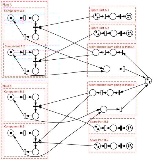
Figure 3.
An example of the expansion of the original GSPN structure.
Once the GSPN model is developed, step 5 of the proposed method consists of performing several simulations, considering different numbers of spare parts for each asset and a different number of maintenance teams. In each new simulation, the average probability of having tokens in each presented place is calculated, as well as the average number of firings of each transition in a given time interval. In this way, it is possible to obtain, for each new scenario/simulation, reliability and availability values for each asset and the systems as a whole.
Such results, together with the financial calculation that involves operating costs (considering costs with managing spare parts inventories and hiring maintenance teams) and revenues associated with generation (and, consequently, dependent on the availability of the system), allow, in step 6 of the method, the most advantageous scenario from an economic point of view to be established.
Finally, it is worth noting that the modularity of the proposed GSPN modeling allows the method to be applicable in several industrial scenarios. The method’s ability to represent the logistical challenges associated with inventory management and maintenance team management makes it particularly interesting in scenarios where such problems are critical, such as in hard-to-reach plants. The case study presented in the following chapter tries to show the advantages of the proposed method in scenarios like this.
4. Case Study
The case study proposed in this work has as primary objective to demonstrate the application of GSPN as a tool to assist in the planning and optimization of maintenance logistics. Due to its technical characteristics, the growth of electricity generation from clean power sources, the need for DERs, and the financial return that can be obtained from such investments, a case study in which two SHPPs are considered was chosen. The data used in this case study were obtained from two SHPPs located in the central region of Brazil, as well as from the literature when necessary.
As proposed by the method previously presented in Section 3, the first step that needs to be taken is to study the systems that will be analyzed. In this case, the two considered SHPPs, named “Plant A” and “Plant B”, are capable of generating, respectively, 25 MW and 29.5 MW. The two plants are located in the same stream, being plant A located upstream from plant B. Each plant has three generating units (Gus), of which the main components considered in this work are the generator, the turbine, the bearings (one radial bearing, on the turbine side, and one combined bearing, on the generator side, which joint the functions of a guide bearing and a thrust bearing), and the control and automation (C&A) system. Functionally there are no differences between the units and, therefore, a single functional tree can represent them, as shown in Figure 4.
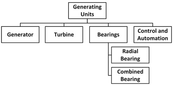
Figure 4.
Generating units’ functional tree.
The second step of the method is the collection of failure and repair data of the considered assets. Often this type of information is not easy to be obtained, especially when dealing with new projects. To overcome the lack of real data, it is possible to resort to literature data sources such as Oreda [29] and seek reference data according to the analyzed equipment and its failure modes. Thus, the considered failure rate for each component is assumed to be represented by an exponential distribution with a parameter λ for all considered components, i.e., the assumption that the failure rate function is constant and independent of time is considered. On the other hand, the generator, turbine, and bearings repair times were estimated from Oreda’s data on active maintenance time, i.e., the calendar time during which maintenance work is carried out on each component, regardless of the number of persons who can work on it [29]. In these cases, the resulting distribution is a two-parameter Weibull distribution with the highest probabilities of the repair time occurring around the mean value. In turn, due to the lack of data related to the control and automation system repair time, the resulting distribution for this component MTTR is exponential.
Once this data collection was carried out for the components presented in Figure 4, the values for the distributions of mean time between failures (MTBF) and mean time to repair (MTTR), respectively shown in Table 1 and Table 2, were determined.

Table 1.
Parameter values of the mean time between failures (MTBF) distributions of the considered components.
Table 2.
Parameter values of the mean time to repair (MTTR) distributions of the considered components.
The third step in the proposed method is the estimation of maintenance team travel time between sites and new spare parts shipping time. Regarding the former, the considered SHPPs are compact facilities with a semi-autonomous operation, leading to a minimal need for in-house personnel. Thus, the operation can be carried out remotely from a headquarters located in a nearby city whose distance is approximately 60 km for Plant A and 70 km for Plant B. Maintenance teams remain in the same headquarters, on standby for any eventuality at the plants while performing routine activities. Thus, in the event of an alarm from the Supervisory Control and Data Acquisition (SCADA) system of one of the plants, one of the maintenance teams available at the headquarters moves to the plant with the unit in a fault condition. The route includes dirt roads and highways, and the travel time between the headquarters and each plant is shown in Figure 5.
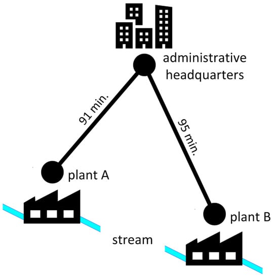
Figure 5.
Travel time between the administrative headquarters and the plants.
In addition to the travel time between the headquarters and the plants, preparation time must be considered for organizing and checking the material and tools needed to carry out repairs at the plant. In this case, it was considered an average preparation time of 120 min. Hence, the total mobilization times are 211 min. for plant A and 215 min. for plant B. Regarding the new spare parts shipping time, a period of 90 days was considered for the interval between the purchase and delivery of the generator and turbine parts and a period of 60 days for the bearing parts, since in these cases parts are manufactured on demand. For the control and automation system parts, a period of 15 days was considered for the purchase and parts’ delivery, since, in this case, they are counterparts.
After collecting the data from steps 2 and 3, the fourth step of the method is the development of the PNs according to the proposed method. Figure 6 presents the GSPN structure used to represent each asset, each spare part, and each maintenance team in the model. The GSPN presented uses the proposed structures to represent the SHPPs under study. In total, there are thirty assets represented, located in the two SHPPs. The arcs in blue (connecting spare parts modules with component modules) and in green (connecting maintenance teams modules with component modules) are colored to try to facilitate the visualization of the GSPN, since the total number of arcs ends up making it difficult to understand. The GSPN was developed in a Petri net software called GRIF [30], which was used to run the model.
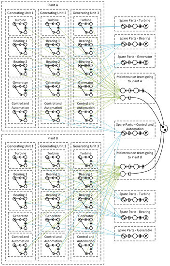
Figure 6.
GSPN structure of the case study.
Once the PN models were developed, different scenarios can be simulated. In this case, 14 different scenarios were considered, in which the number of spare parts initially in stock for each main component (control and automation system, generator, turbine, and bearings) and the number of contracted maintenance teams varies. For instance, scenario S1 considered the availability of only one maintenance team and that all components would have only one set of spare parts available; the other scenarios are variations of this scenario. Scenario S2, e.g., maintains the same number of spare parts for each considered component in scenario S1, but the number of available maintenance teams initially considered is doubled. All other scenarios consider the availability of only one maintenance team, but there are variations in the number of spare parts available for each main component. Scenarios S3, S4, S5, and S6 consider, in each case, that only one considered component has two sets of spare parts available, while the other components keep only one set of spare parts available; in turn, scenarios S7, S8, S9, and S10 consider, respectively, that one of the considered components do not have spare parts available, while the others keep only one set of spare parts available. Scenario S11 considers the lack of available spare parts for all components, scenario S12 states that only the control and automation system has spare parts, and scenario S13 considers that only the control and automation system and the bearings have spare parts available. Finally, scenario S14 considers that all the main components have two sets of spare parts each.
The criterion used to compare the results of each of these scenarios will be the financial return obtained in each case. However, some assumptions must be considered concerning such simulations. As mentioned before, the GUs of each plant do not have functional differences, being composed of the same assets. However, due to the difference in the power generated by the two plants, the designs of the GUs of each plant are not the same. Therefore, the spare parts related to the generator, turbine, and bearings are not interchangeable between the plants’ units. Besides, the replacement parts of these components occupy a significant area for proper storage and require some care in transportation. These features make their storage more suitable if carried out in the plants’ warehouses.
On the other hand, regarding the control and automation system, the same components (such as sensors, actuators, and programmable logic controllers) can be used in the units of both plants. Furthermore, these counterpart pieces occupy a small storage area. Therefore, the replacement parts of this subsystem can be kept in a single warehouse at the administrative headquarters.
In addition, a two-year simulation period was considered, with the results being extrapolated to a 25-year concession period for both power plants. These two years are considered to be the duration of an SHPP UG’s operational campaign. Thus, every two years, a preventive general overhaul would be carried out at the plants’ units and, therefore, failures that occur during this period are considered as unforeseen failures, directly affecting the availability of the units. After each biannual maintenance, maintained components are considered to be returned to an as-good-as-new condition.
Some hypotheses related to values and costs were also raised so that the simulations could be performed. Based on the Brazilian domestic market, an operating cost of USD 5.00 per MWh generated is considered. Likewise, the considered revenue value per MWh generated is USD 20.00, leading to an operational incoming of USD 15.00 per MWh generated.
The cost of each maintenance team, consisting of five individuals (two mechanical technicians, two electrical technicians, and an electronics technician) is USD 50.00 per hour. As part of the company’s permanent staff, it is considered a work regime of 40 h per week during the entire period analyzed for the maintenance teams. Labor and additional costs, such as overtime, are considered covered by this amount.
The initial investment considered for each plant, excluding spare parts, is 30 million US dollars. In turn, the considered unitary investment of spare parts for each component is given in Table 3.
Table 3.
Spare parts unitary investment for each component.
The unit values of spare parts refer to a complete set of parts that make up one unit of each component (in the case of bearings, a radial bearing and a combined bearing). In the event of a failure that requires the replacement of one of the pieces of equipment, it is accepted that the purchase request for its replacement in stock is made immediately after the maintenance of the equipment. The cost of such replacement is considered as part of the operating cost since the amount involved in the replacement of a single part is significantly less than the cost of the entire component. Besides, costs of disposing of waste and broken pieces are considered as part of the operating cost as well.
It is important to have in mind that all these values may vary according to the application and, as mentioned earlier, they were estimated to show the capacity of the proposed method. It is recommended that, before the method application, a more detailed investigation regarding such values should be carried out. Furthermore, given the good practices originally applied to the optimization modeling of energy systems [31], the proposed approach does not aim to accurately forecast the operation of complex systems from a set of quantitative results, but rather to assist in the development of the maintenance planning based on insights and reasoning stimulated by the results obtained.
Having said that, the simulations result for the 14 considered scenarios (S1 to S14) in this work are presented in Table 4. Figure 7, in turn, presents the expected profit for each simulated scenario.
Table 4.
Simulation results for the 14 scenarios considered.
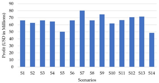
Figure 7.
Overall expected profit for each simulated scenario.
It is interesting to note some aspects concerning the results presented. Considering the profitability criterion of each scenario, e.g., it is clear that the most advantageous scenario is scenario 7 (S7), while the least advantageous scenario is scenario 14 (S14). However, the latter is the scenario in which the greatest output power is obtained, i.e., it is the scenario with the greatest availability of the plants’ GUs. On the other hand, scenario 4 (S4) is a scenario whose financial return is intermediate between the values of S7 and S14, presenting, at the same time, the expected availability practically identical to that of scenario 14. The greater availability, in these cases, is obtained due to the greater number of spare parts available, but the cost associated with such mobilization ends up causing the enterprise’s return to be reduced compared to the most profitable scenario.
That is, considering the financial return as the only parameter for choosing the best scenario, although scenario 7 allows a total power generated over the 25 years of concession just close to the average value considering all scenarios (S7 has an output power of 10,392,472 MWh, while the average value considering the 14 scenarios is 10,243,466 MWh), the number of spare parts and maintenance teams become optimized in this case. It is also worth mentioning that in scenario 7 there is no provision for spare parts for the turbine, which among the components considered would be the one with the highest unit value.
5. Conclusions
This work aimed to present an application of GSPNs as a modeling tool to optimize and plan the most efficient maintenance logistics approach for a DER project with two SHPPs managed by the same company, taking into account aspects related to the availability of spare parts and the sharing of maintenance teams.
From this modeling, several scenarios were simulated in which the number of spare parts of each component was considered and the number of maintenance teams available to work in the plants varied to verify the condition in which the financial return of the project would be maximized.
Some strong hypotheses and considerations needed to be made concerning the values of spare parts, operating costs, costs of maintenance teams, sales value of the MWh generated, among other aspects, to enable the simulations and demonstrate the proposed method. The use of such hypotheses sought to balance the cost-benefit of the analysis performed, keeping it as simple as possible and as complex as necessary. In addition, following the same best practice applied for energy system optimization modeling, the proposed approach is not intended to accurately forecast the operation of complex facilities, such as DERs, but rather to assist in the development of maintenance planning based on insights and reasoning stimulated by the results obtained. Therefore, such hypotheses do not affect the validity of the method and, in addition, in applications that more detailed economic and financial analysis can be considered a priori, such values could be obtained with better accuracy and precision. The method application must be verified on a case-by-case basis. However, the GSPN proposed structures, especially concerning the transitions and places of the representations of components, spare parts, and displacement of teams, can be considered the same, independently of the analyzed system.
From the results obtained, it is possible to notice the capability and robustness of the proposed method. In the case study presented and having the financial return obtained in each scenario as the only criterion for evaluating the results, it was possible to determine the ideal number of maintenance teams and spare parts for each component. Furthermore, the results demonstrate how previously established ideas that could be considered reasonable at first sight are not confirmed, such as considering that the financial return should be maximized from greater availability of the generating units. For instance, it is interesting to note that although the scenario considered ideal, S7, is the one that allows the greatest financial return, it is not the one that has the greatest availability of GUs, i.e., it is not the one that maximizes the output power.
Another aspect that must be taken into account is the use of the financial return as a single value to evaluate the proposed approach and classify the best scenario. This aspect makes the analysis of the results more restricted, although it does not invalidate the application of the GSPN as a tool for the proposed modeling. Bearing this in mind, as a proposal for future works, a natural evolution of the work elaborated in this article could be developed by incorporating a multiple-criteria decision making (MCDM) technique into the developed method, in which not only the profit obtained with the different scenarios would be considered, but also other aspects of interest could be included in the analysis.
Author Contributions
Conceptualization, A.H.d.A.M., M.A.d.C.M., C.A.M., A.C.N. and G.F.M.d.S.; Data curation, A.H.d.A.M. and M.A.d.C.M.; Formal analysis, A.H.d.A.M., M.A.d.C.M. and G.F.M.d.S.; Funding acquisition, G.F.M.d.S.; Investigation, A.H.d.A.M., M.A.d.C.M. and G.F.M.d.S.; Methodology, A.H.d.A.M., M.A.d.C.M., C.A.M., A.C.N. and G.F.M.d.S.; Project administration, G.F.M.d.S.; Resources, G.F.M.d.S.; Supervision, G.F.M.d.S.; Validation, M.A.d.C.M., C.A.M., A.C.N. and G.F.M.d.S.; Visualization, A.H.d.A.M., M.A.d.C.M. and G.F.M.d.S.; Writing—original draft, A.H.d.A.M., M.A.d.C.M., C.A.M., A.C.N. and G.F.M.d.S.; Writing—review and editing, A.H.d.A.M., M.A.d.C.M. and G.F.M.d.S. All authors have read and agreed to the published version of the manuscript.
Funding
This research was funded by Fundação para o Desenvolvimento Tecnológico da Engenharia (FDTE) and EDP Brasil as part of an ANEEL R&D Project (project number PD-0069-0017/2017), and Conselho Nacional de Desenvolvimento Científico e Tecnológico (CNPq), founding number 153383/2016-0.
Conflicts of Interest
The authors declare no conflict of interest. The funders had no role in the design of the study; in the collection, analyses, or interpretation of data; in the writing of the manuscript, or in the decision to publish the results.
References
- IEA. World Energy Outlook; IEA: Paris, France, 2021. [Google Scholar]
- EIA. Annual Energy Outlook 2022; EIA: Washington, DC, USA, 2022.
- Jung, S.; Bae, Y.; Kim, J.; Joo, H.; Kim, H.; Jung, J. Analysis of Small Hydropower Generation Potential: (1) Estimation of the Potential in Ungaged Basins. Energies 2021, 14, 2977. [Google Scholar] [CrossRef]
- Jung, J.; Jung, S.; Lee, J.; Lee, M.; Kim, H.S. Analysis of Small Hydropower Generation Potential: (2) Future Prospect of the Potential under Climate Change. Energies 2021, 14, 3001. [Google Scholar] [CrossRef]
- Kishore, T.S.; Patro, E.R.; Harish, V.S.K.V.; Haghighi, A.T. A Comprehensive Study on the Recent Progress and Trends in Development of Small Hydropower Projects. Energies 2021, 14, 2882. [Google Scholar] [CrossRef]
- Donovan, C.; Fomicov, M.; Gerdes, L.-K.; Waldron, M. Energy Investing: Exploring Risk and Return in the Capital Markets; IEA: Paris, France, 2020. [Google Scholar]
- Caminada Netto, A.; Melani, A.H.A.; Murad, C.A.; Nabeta, S.I.; de Souza, G.F.M. Petri Net Based Reliability Analysis of Thermoelectric Plant Cooling Tower System: Effects of Operational Strategies on System Reliability and Availability. In Proceedings of the Joint ICVRAM ISUMA UNCERTAINTIES Conference, Florianópolis, Brazil, 8–11 April 2018; p. 13. [Google Scholar]
- Murad, C.A.; de Melani, A.H.A.; de Michalski, M.A.C.; Netto, A.C.; de Souza, G.F.M. Estimation of Operational and Maintenance Tasks Influence on Equipment Availability Through Petri Net Modeling. In Proceedings of the 2020 Annual Reliability and Maintainability Symposium (RAMS), Palm Springs, CA, USA, 27–30 January 2020; IEEE: Piscataway, NJ, USA, 2020; pp. 1–6. [Google Scholar]
- Melani, A.H.A.; Murad, C.A.; Netto, A.C.; Souza, G.F.M.; Nabeta, S.I. Maintenance Strategy Optimization of a Coal-Fired Power Plant Cooling Tower through Generalized Stochastic Petri Nets. Energies 2019, 12, 1951. [Google Scholar] [CrossRef] [Green Version]
- Santos, F.P.; Teixeira, Â.P.; Soares, C.G. Modeling, Simulation and Optimization of Maintenance Cost Aspects on Multi-Unit Systems by Stochastic Petri Nets with Predicates. Simulation 2019, 95, 461–478. [Google Scholar] [CrossRef]
- Silva, M. 50 Years after the PhD Thesis of Carl Adam Petri: A Perspective. IFAC Proc. Vol. 2012, 45, 13–20. [Google Scholar] [CrossRef] [Green Version]
- Kang, C.W.; Imran, M.; Omair, M.; Ahmed, W.; Ullah, M.; Sarkar, B. Stochastic-Petri Net Modeling and Optimization for Outdoor Patients in Building Sustainable Healthcare System Considering Staff Absenteeism. Mathematics 2019, 7, 499. [Google Scholar] [CrossRef] [Green Version]
- Reisig, W.; Petri, C.A. Carl Adam Petri: Ideas, Personality, Impact; Reisig, W., Rozenberg, G., Eds.; Springer International Publishing: Cham, Switzerland, 2019; ISBN 978-3-319-96153-8. [Google Scholar]
- Elusakin, T.; Shafiee, M.; Adedipe, T.; Dinmohammadi, F. A Stochastic Petri Net Model for O&M Planning of Floating Offshore Wind Turbines. Energies 2021, 14, 1134. [Google Scholar]
- Peng, L.; Xie, P.; Tang, Z.; Liu, F. Modeling and Analyzing Transmission of Infectious Diseases Using Generalized Stochastic Petri Nets. Appl. Sci. 2021, 11, 8400. [Google Scholar] [CrossRef]
- Marsan, M.A. Stochastic Petri Nets: An Elementary Introduction. In Advances in Petri Nets 1989; Rozenberg, G., Ed.; Springer: Berlin/Heidelberg, Germany, 1990; pp. 1–29. ISBN 3540524940. [Google Scholar]
- Bause, F.; Kritzinger, P.S. Stochastic Petri Nets: An Introduction to the Theory, 2nd ed.; Vieweg+Teubner Verlag: Wiesbaden, Germany, 2002; ISBN 978-3528155353. [Google Scholar]
- Murata, T. Petri Nets: Properties, Analysis and Applications. Proc. IEEE 1989, 77, 541–580. [Google Scholar] [CrossRef]
- Dingle, N.J.; Knottenbelt, W.J. Automated Customer-Centric Performance Analysis of Generalised Stochastic Petri Nets Using Tagged Tokens. Electron. Notes Theor. Comput. Sci. 2009, 232, 75–88. [Google Scholar] [CrossRef] [Green Version]
- Wu, W.; Bu, B. Security Analysis for CBTC Systems under Attack-Defense Confrontation. Electronics 2019, 8, 991. [Google Scholar] [CrossRef] [Green Version]
- Schmidt, M.; Weik, N.; Zieger, S.; Schmeink, A.; Nießen, N. A Generalized Stochastic Petri Net Model for Performance Analysis of Trackside Infrastructure in Railway Station Areas under Uncertainty. In Proceedings of the 2019 IEEE Intelligent Transportation Systems Conference, ITSC 2019, Auckland, New Zealand, 27–30 October 2019; pp. 3732–3737. [Google Scholar] [CrossRef]
- Konopko, J. A Petri Net Model for Distributed Energy System. In Proceedings of the International Conference of Computational Methods in Sciences and Engineering 2015, ICCMSE 2015, Athens, Greece, 20–23 March 2015; Volume 1702, p. 070003. [Google Scholar]
- Melani, A.H.A.; Silva, J.M.; de Souza, G.F.M.; Silva, J.R. Fault Diagnosis Based on Petri Nets: The Case Study of a Hydropower Plant. IFAC-PapersOnLine 2016, 49, 1–6. [Google Scholar] [CrossRef]
- Mansour, M.M.; Wahab, M.A.A.; Soliman, W.M. Petri Nets for Fault Diagnosis of Large Power Generation Station. Ain Shams Eng. J. 2013, 4, 831–842. [Google Scholar] [CrossRef] [Green Version]
- Mahdi, I.; Chalah, S.; Nadji, B. Reliability Study of a System Dedicated to Renewable Energies by Using Stochastic Petri Nets: Application to Photovoltaic (PV) System. Energy Procedia 2017, 136, 513–520. [Google Scholar] [CrossRef]
- Chang, C.-K.; Hsiang, C.-L. An Optimal Maintenance Policy Based on Generalized Stochastic Petri Nets and Periodic Inspection. Asian J. Control 2010, 12, 364–376. [Google Scholar] [CrossRef]
- Santos, F.P.; Teixeira, A.P.; Guedes Soares, C. Maintenance Planning of an Offshore Wind Turbine Using Stochastic Petri Nets With Predicates. J. Offshore Mech. Arct. Eng. 2018, 140, 021904. [Google Scholar] [CrossRef]
- Batelić, J.; Griparić, K.; Matika, D. Impact of Remediation-Based Maintenance on the Reliability of a Coal-Fired Power Plant Using Generalized Stochastic Petri Nets. Energies 2021, 14, 5682. [Google Scholar] [CrossRef]
- OREDA. OREDA: Offshore Reliability Data-Volume 1-Topside Equipment, 5th ed.; OREDA Participants: Trondheim, Norway, 2009; ISBN 978-82-14-04830-8. [Google Scholar]
- SATODEV. GRIF Software. Available online: https://www.satodev.com/ (accessed on 31 January 2019).
- DeCarolis, J.; Daly, H.; Dodds, P.; Keppo, I.; Li, F.; McDowall, W.; Pye, S.; Strachan, N.; Trutnevyte, E.; Usher, W.; et al. Formalizing Best Practice for Energy System Optimization Modelling. Appl. Energy 2017, 194, 184–198. [Google Scholar] [CrossRef] [Green Version]
Publisher’s Note: MDPI stays neutral with regard to jurisdictional claims in published maps and institutional affiliations. |
© 2022 by the authors. Licensee MDPI, Basel, Switzerland. This article is an open access article distributed under the terms and conditions of the Creative Commons Attribution (CC BY) license (https://creativecommons.org/licenses/by/4.0/).