
Data Screening Based on Correlation Energy Fluctuation Coefficient and Deep Learning for Fault Diagnosis of Rolling Bearings


Abstract
:1. Introduction
2. Intelligent Identification Method
2.1. Data Cleaning
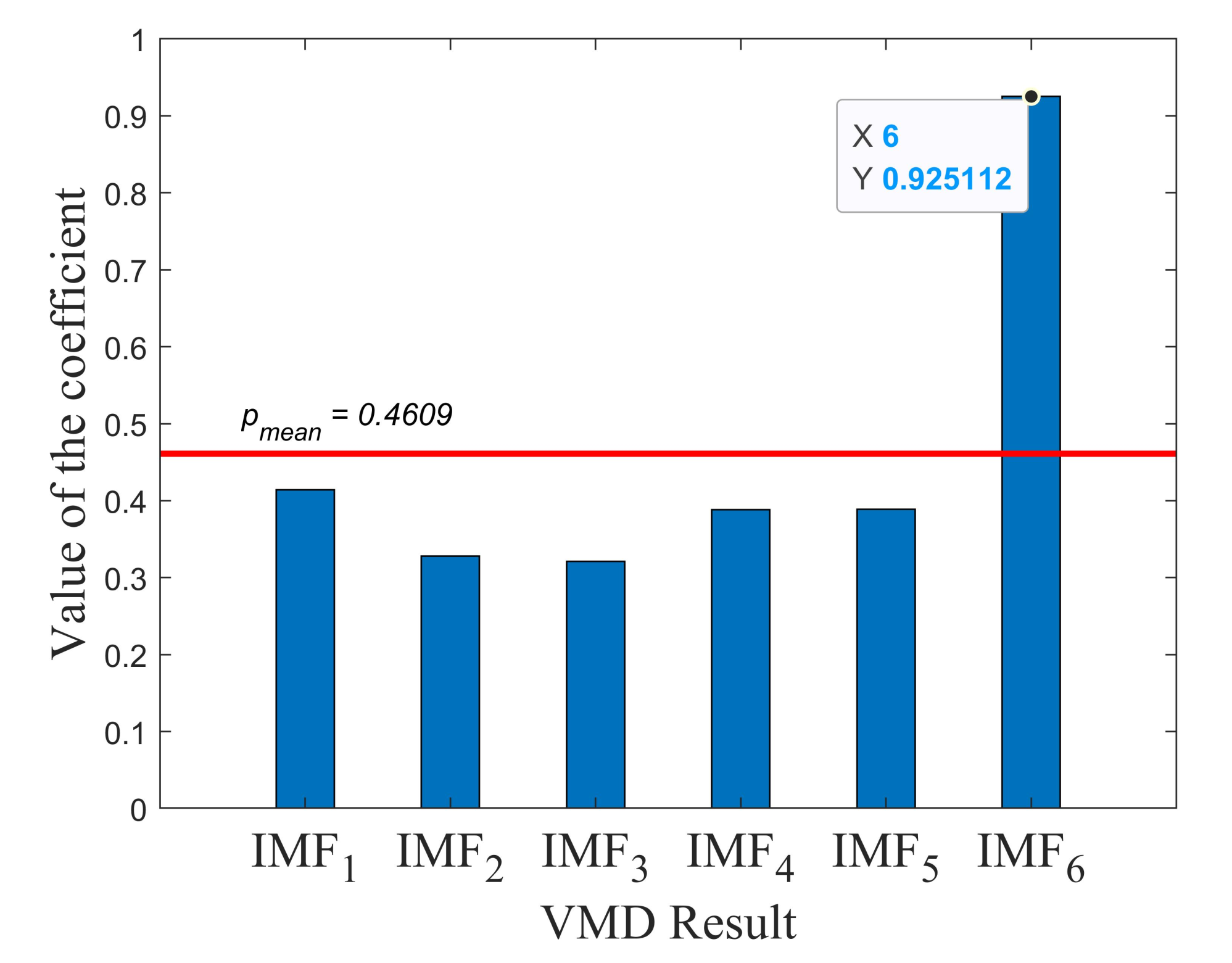
2.1.1. Principle of Evaluation
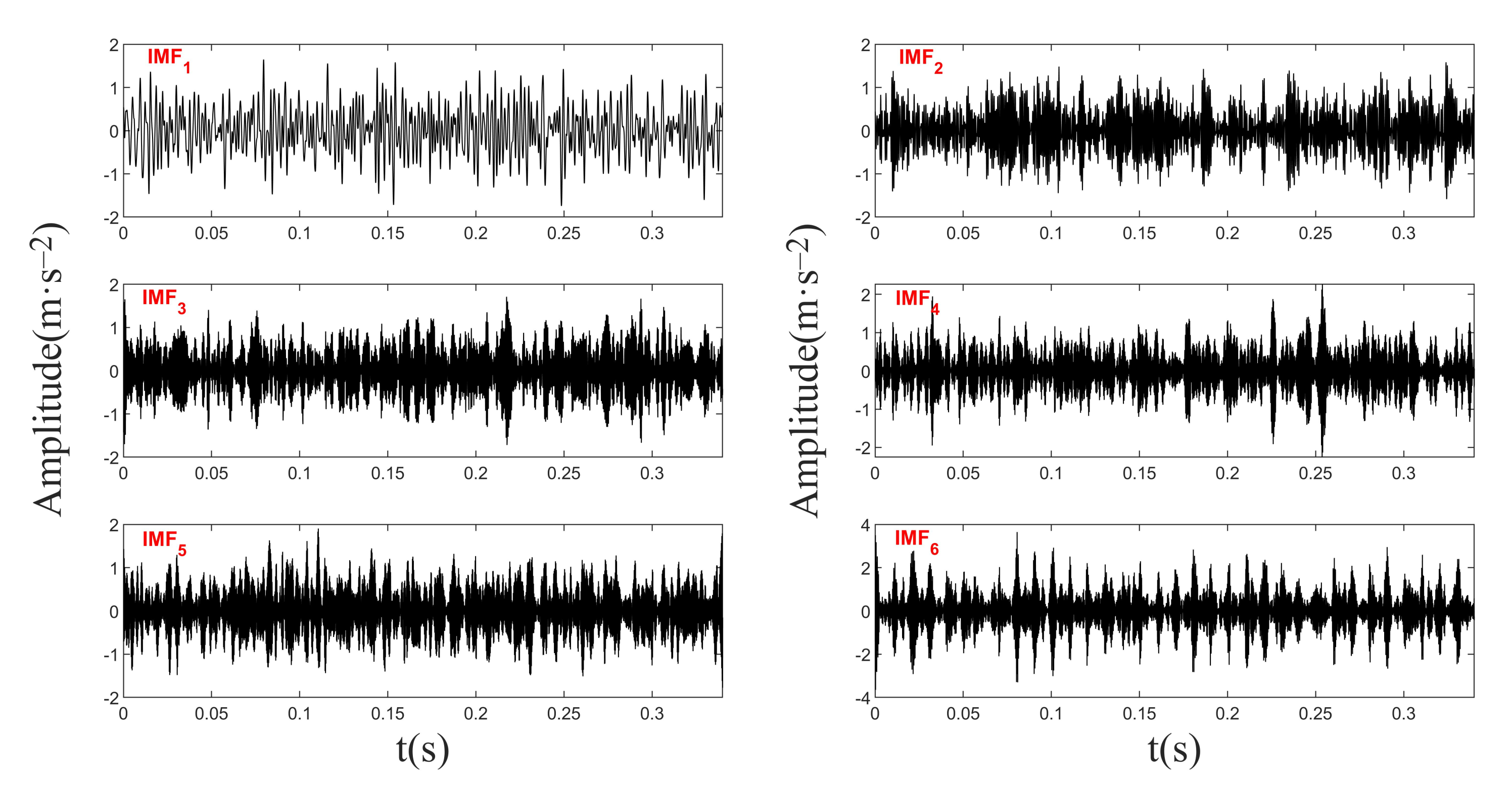
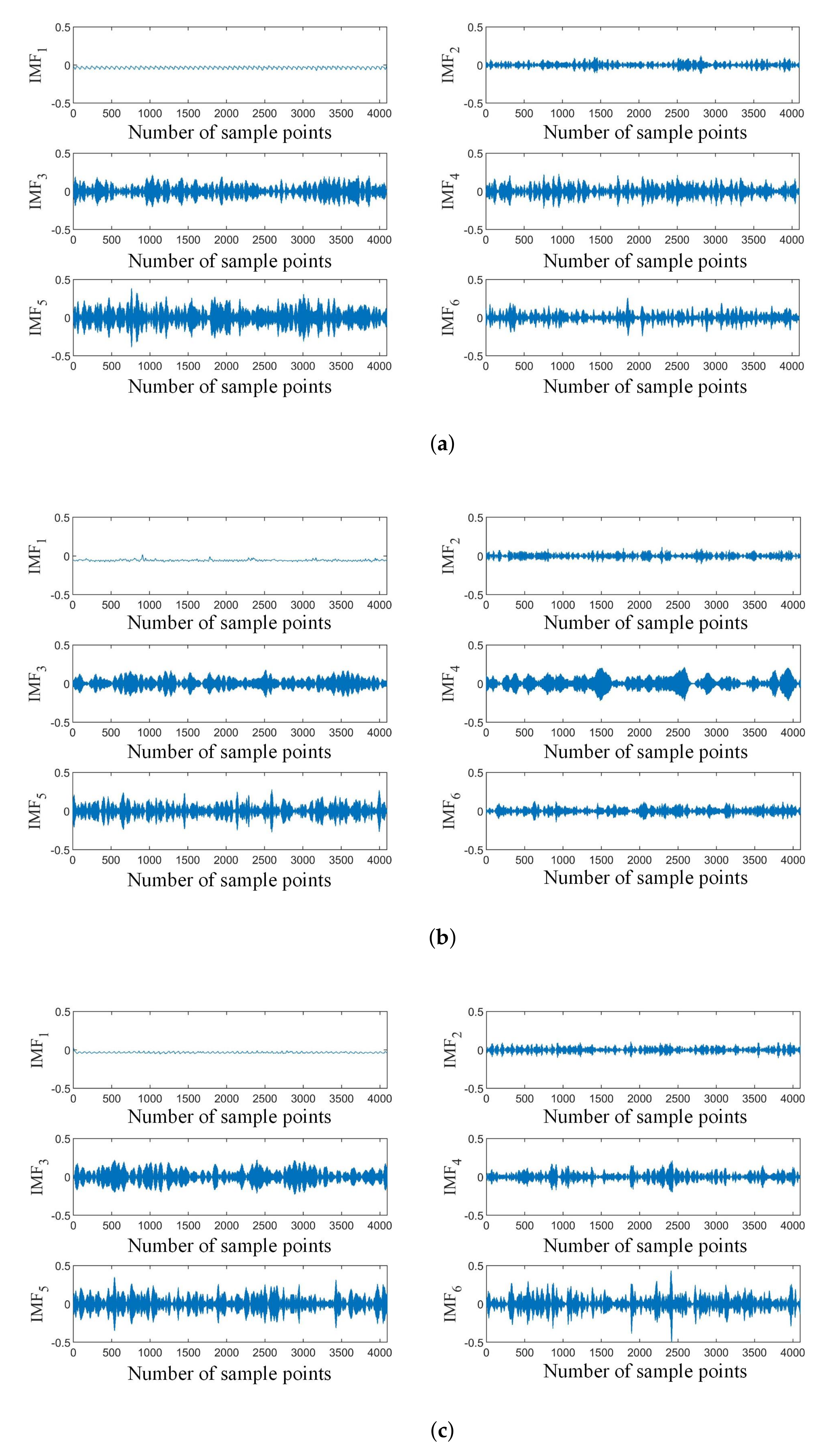
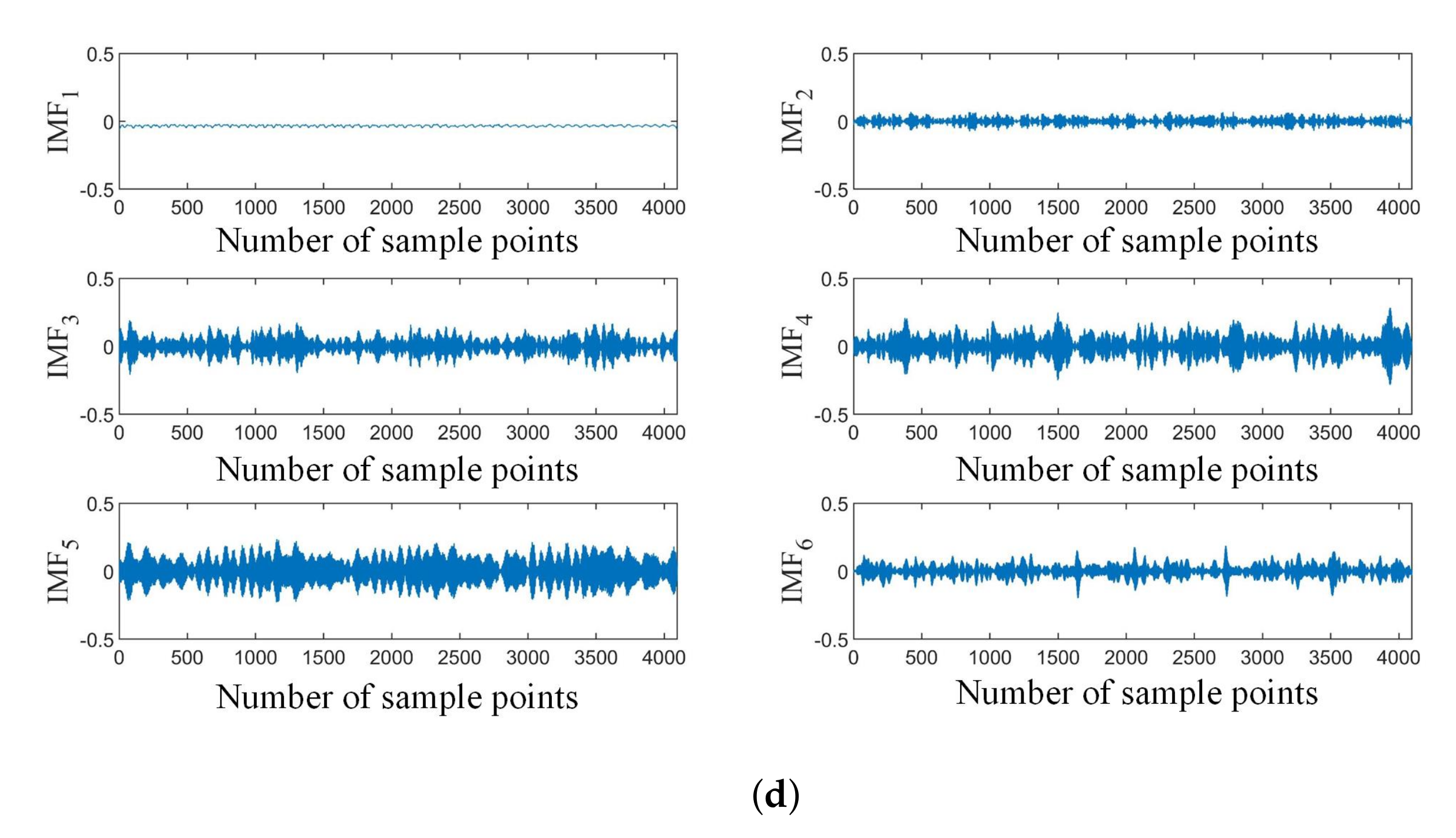
2.1.2. Screening and Reconstruction of IMF Components
2.2. Intelligent Diagnosis Model
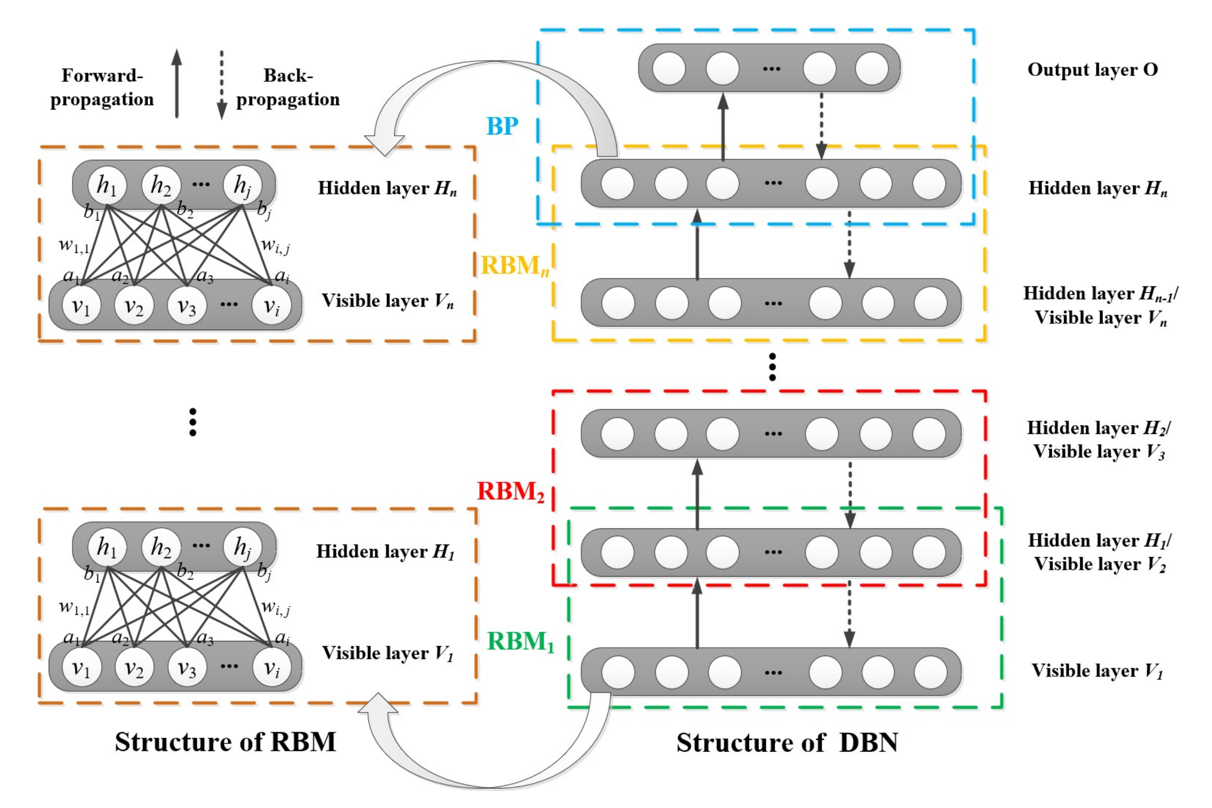
2.2.1. DBN Network Model
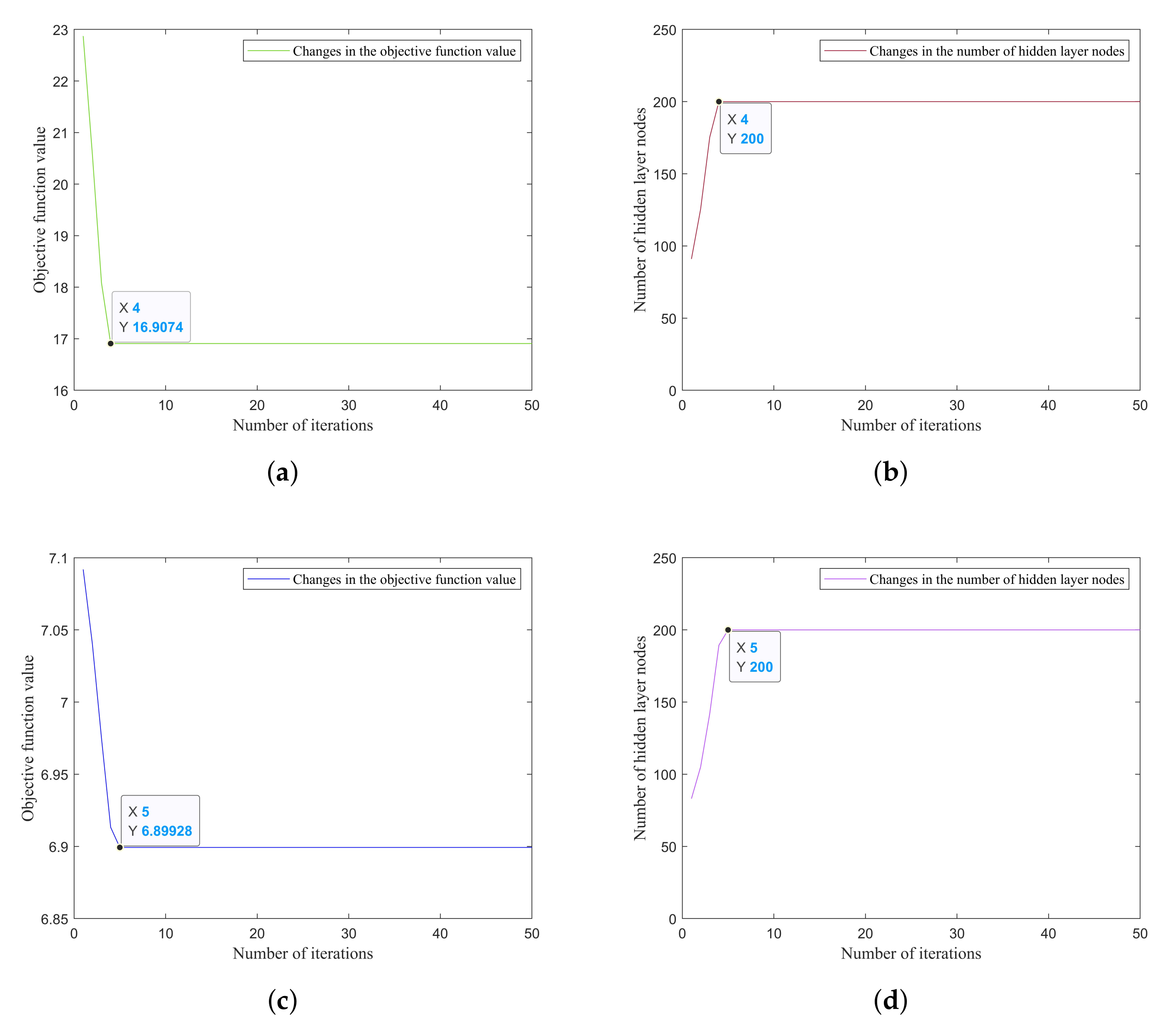
2.2.2. IPSO Optimizes the Structure Parameters of DBN
3. Experimental Analysis and Validation
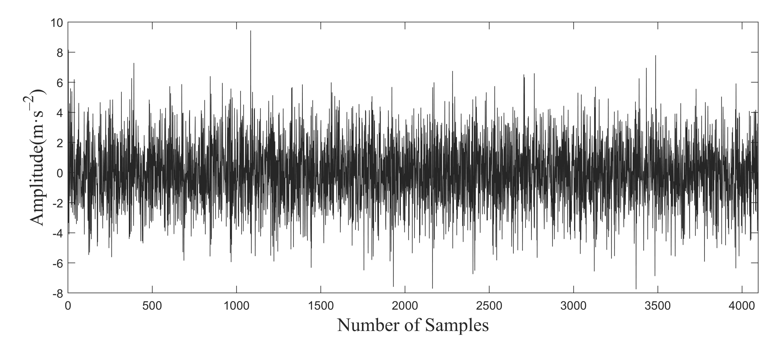
3.1. Validation by Simulated Signal
3.2. Validation by Bench Test
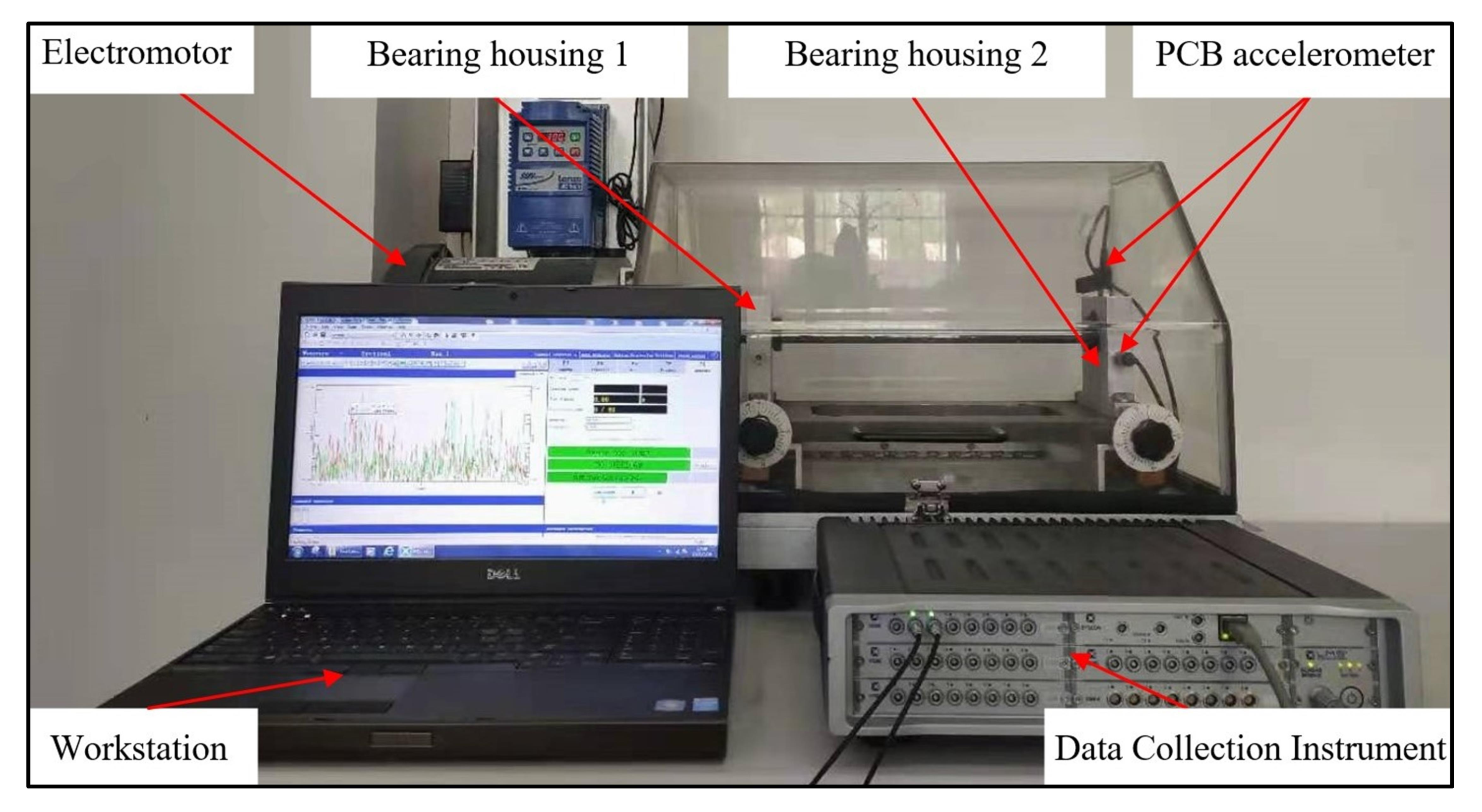
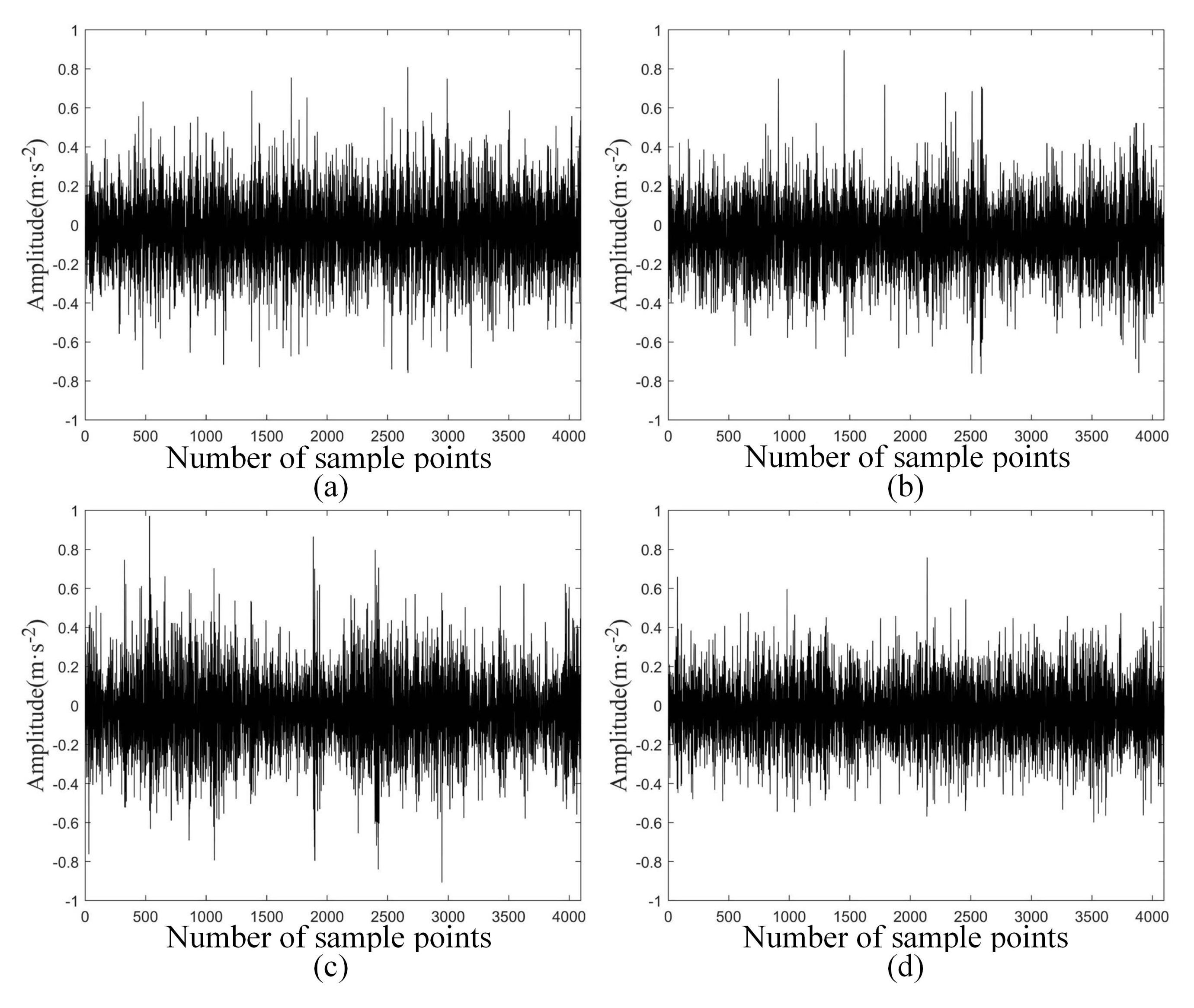
3.2.1. Test System Construction and Signal Acquisition
3.2.2. Data Cleaning of Bench Test
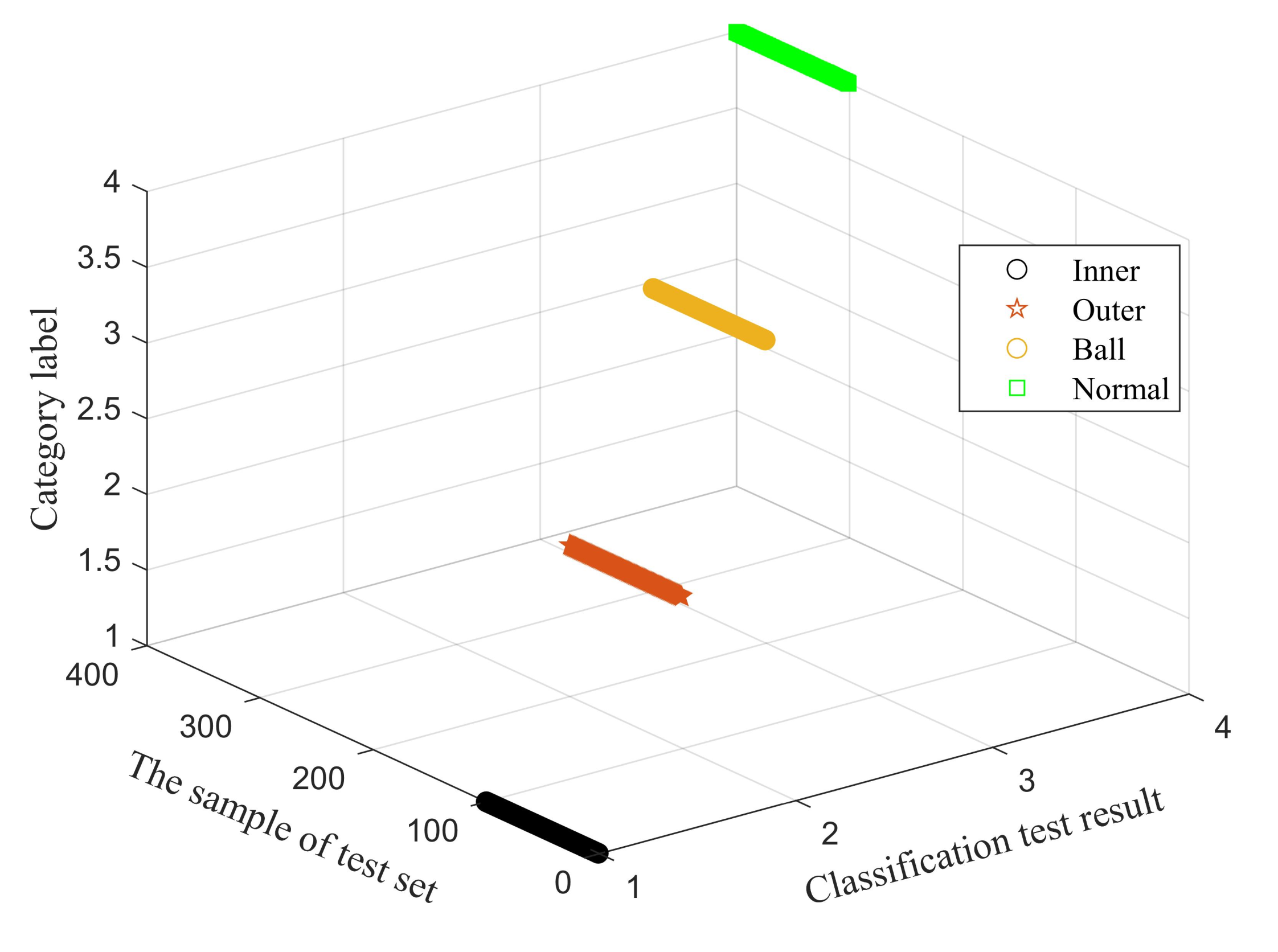
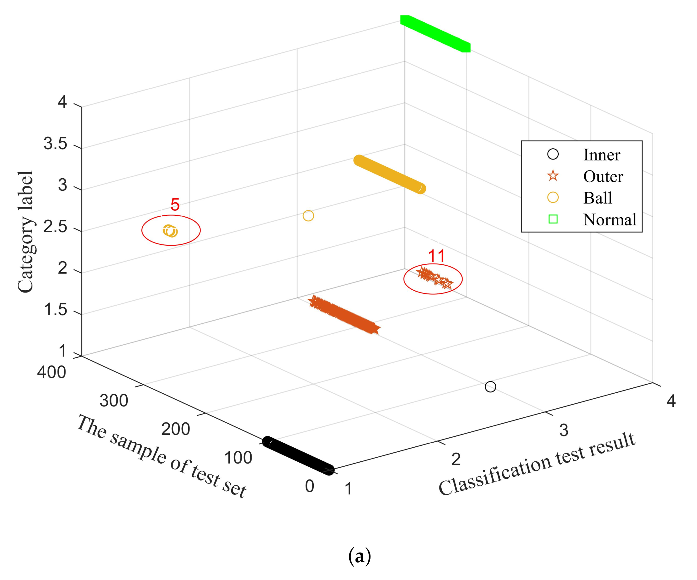
3.2.3. Intelligent State Identification of Bearing Based on DBN Optimized by IPSO
4. Conclusions
Author Contributions
Funding
Acknowledgments
Conflicts of Interest
References
- Liu, J.; Xu, Z.; Zhou, L.; Yu, W.; Shao, Y. A statistical feature investigation of the spalling propagation assessment for a ball bearing. Mech. Mach. Theory 2019, 131, 336–350. [Google Scholar] [CrossRef]
- Rubini, R. Application of the envelope and wavelet transform analyses for the diagnosis of incipient faults in ball bearing. Mech. Syst. Signal Process. 2001, 15, 287–302. [Google Scholar] [CrossRef]
- Qin, Y.; Li, W.T.; Yuen, C.; Tushar, W.; Saha, T. IIoT-enabled health monitoring for integrated heat pump system using Mixture Slow Feature Analysis. IEEE Trans. Inf. Inform. 2021. [Google Scholar] [CrossRef]
- Huang, N.E.; Shen, Z.; Long, S.R.; Wu, M.C.; Shih, H.H.; Zheng, Q.; Yen, N.-C.; Tung, C.C.; Liu, H.H. The empirical mode decomposition and the Hilbert speetrum for nonlinear and nonstationary time series analysis. Proc. Math. Phys. Eng. Sci. 1998, 454, 903–995. [Google Scholar] [CrossRef]
- Wu, Z.; Huang, N.E. Ensemble empirical mode decomposition: A noise-assisted data analysis method. Adv. Adapt. Data Anal. 2009, 1, 1–41. [Google Scholar] [CrossRef]
- Smith, J.S. The local mean decomposition and its application to EEG perception data. J. R. Soc. Interface 2005, 2, 443–454. [Google Scholar] [CrossRef]
- Dragomiretskiy, K.; Zosso, D. Variational mode decomposition. IEEE Trans. Signal Process. 2014, 62, 531–544. [Google Scholar] [CrossRef]
- Li, H.; Liu, T.; Wu, X.; Chen, Q. Application of EEMD and improved frequency band entropy in bearing fault feature extraction. ISA Trans. 2019, 88, 170–185. [Google Scholar] [CrossRef]
- Li, H.; Liu, T.; Wu, X.; Chen, Q. Application of optimized variational mode decomposition based on kurtosis and resonance frequency in bearing fault feature extraction. Trans. Inst. Meas. Control 2019, 42, 518–527. [Google Scholar] [CrossRef]
- Zhao, L.; Yu, W.; Yan, R. Rolling Bearing Fault Diagnosis Based on CEEMD and Time Series Modeling. Math. Probl. Eng. 2014, 2014, 101867. [Google Scholar] [CrossRef]
- Zhang, C.; Yao, W.; Deng, W. Fault Diagnosis for Rolling Bearings Using Optimized Variational Mode Decomposition and Resonance Demodulation. Entropy 2020, 22, 739. [Google Scholar] [CrossRef]
- Wang, H.D.; Deng, S.E.; Yang, J.X.; Liao, H.; Li, W.B. Parameter-Adaptive VMD Method Based on BAS Optimization Algorithm for Incipient Bearing Fault Diagnosis. Math. Probl. Eng. 2020, 2020, 5659618. [Google Scholar] [CrossRef] [Green Version]
- Li, X.; Yang, Y.; Pan, H.; Cheng, J.; Cheng, J. A novel deep stacking least squares support vector machine for rolling bearing fault diagnosis. Comput. Ind. 2019, 110, 36–47. [Google Scholar] [CrossRef]
- Zhou, S.; Qian, S.; Chang, W.; Xiao, Y.; Cheng, Y. A Novel Bearing Multi-Fault Diagnosis Approach Based on Weighted Permutation Entropy and an Improved SVM Ensemble Classifier. Sensors 2018, 18, 1934. [Google Scholar] [CrossRef] [PubMed] [Green Version]
- Dong, W.; Zhang, S.; Jiang, A.; Jiang, W.; Zhang, L.; Hu, M. Intelligent Fault Diagnosis of Rolling Bearings Based on Refined Composite Multi-Scale Dispersion q-Complexity and Adaptive Whale Algorithm-Extreme Learning Machine. Measurement 2021, 176, 108977. [Google Scholar] [CrossRef]
- Luo, M.; Li, C.; Zhang, X.; Li, R.; An, X. Compound feature selection and parameter optimization of ELM for fault diagnosis of rolling element bearings. ISA Trans. 2016, 65, 556–566. [Google Scholar] [CrossRef] [PubMed]
- Li, J.; Yao, X.; Wang, X.; Yu, Q.; Zhang, Y. Multiscale local features learning based on BP neural network for rolling bearing intelligent fault diagnosis. Measurement 2019, 153, 107419. [Google Scholar] [CrossRef]
- Hinton, G.E.; Salakhutdinov, R.R. Reducing the dimensionality of data with neural networks. Science 2006, 313, 504–507. [Google Scholar] [CrossRef] [PubMed] [Green Version]
- Hinton, G.E.; Osindero, S.; Teh, Y.W. A fast learning algorithm for deep belief nets. Neural Comput. 2006, 18, 1527–1554. [Google Scholar] [CrossRef] [PubMed]
- Li, Y.; Wang, L.; Jiang, L. Rolling bearing fault diagnosis based on DBN algorithm improved with PSO. J. Vib. Shock 2020, 39, 89–96. [Google Scholar]
- Qin, B.; Sun, G.D.; Zhang, L.Q.; Liu, Y.L.; Zhang, C.; Wang, J.G. Study on the Rolling Bearing Fault Diagnosis based on the Hilbert Envelope Spectrum Singular Value and IPSO-SVM. J. Mech. Transm. 2017, 41, 166–171. [Google Scholar]


| Amplitude of shock at bearing fault location (A) | 5 |
| Amplitude of Gaussian noise () | 2 |
| Natural frequency of bearing vibration (Hz) () | 4500 |
| Attenuation coefficient () | 800 |
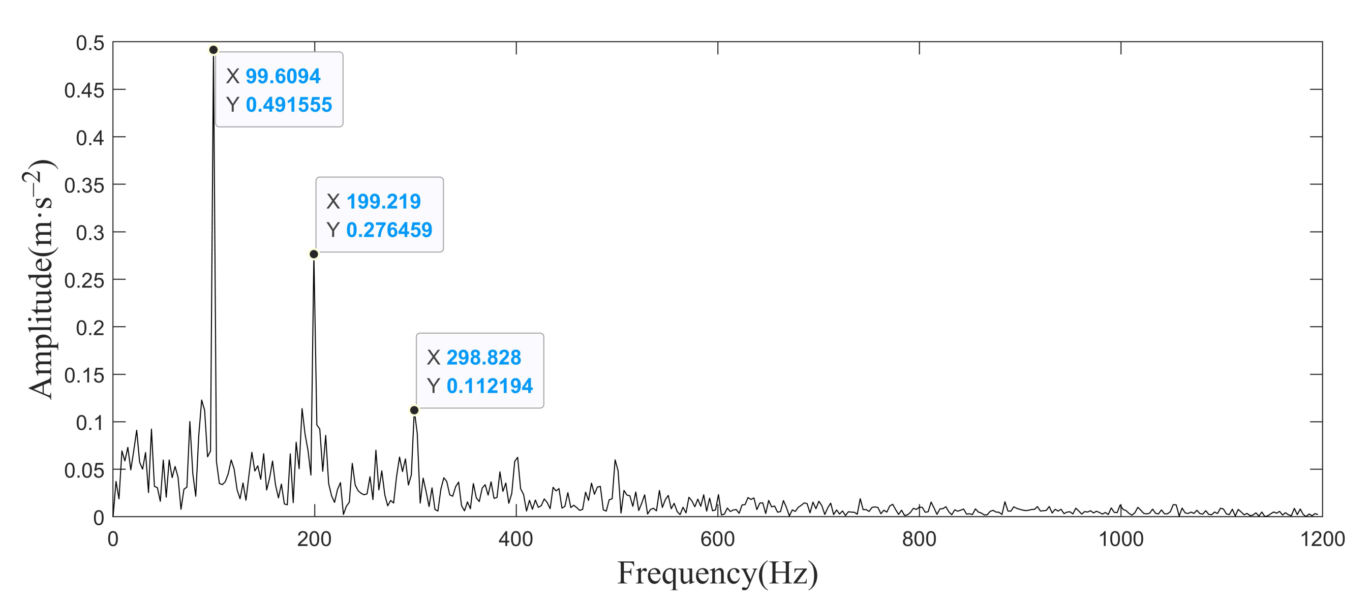
| Characteristic frequency (Hz) () | 100 |
| Sampling frequency (Hz) () | 12,000 |
| Sampling points | 4096 |
| IMF | 0.4140 |
| IMF | 0.3281 |
| IMF | 0.3211 |
| IMF | 0.3884 |
| IMF | 0.3889 |
| IMF | 0.9251 |
| Bearing inner diameter (mm) | 19 |
| Bearing outer diameter (mm) | 47 |
| Number of rolling elements | 8 |
| Rolling element diameter (mm) | 7.9 |
| Pitch circle diameter (mm) | 33.5 |
| Contact angle (deg.) | 0 |
| State Type | Sample Number | Sample Data Volume | ||||||
|---|---|---|---|---|---|---|---|---|
| 1 | 2 | 3 | ··· | 2046 | 2047 | 2048 | ||
| Inner | 1 | 2.939 × | 5.375 × | 7.977 × | 1.800 × | 1.700 × | 1.800 × | |
| ··· | ||||||||
| 300 | 1.479 × | 4.698 × | 4.898 × | 1.637 × | 1.102 × | 5.767 × | ||
| Outer | 1 | 3.167 × | 6.216 × | 1.001 × | 2.743 × | 4.496 × | 5.377 × | |
| ··· | ||||||||
| 300 | 1.123 × | 1.681 × | 2.521 × | 7.721 × | 6.835 × | 6.333 × | ||
| Ball | 1 | 1.001 × | 2.001 × | 2.921 × | 2.335 × | 8.175 × | 1.297 × | |
| ··· | ||||||||
| 300 | 2.881 × | 5.758 × | 8.707 × | 1.600 × | 1.500 × | 1.400 × | ||
| Normal | 1 | 1.042 × | 2.093 × | 3.048 × | 7.573 × | 7.707 × | 7.095 × | |
| ··· | ||||||||
| 300 | 3.142 × | 6.281 × | 9.567 × | 1.200 × | 1.100 × | 1.100 × | ||
| Method | Type | Average | |||
|---|---|---|---|---|---|
| Inner | Outer | Ball | Normal | ||
| After preprocessing and the node combination is [200, 200] | 100% | 100% | 100% | 100% | 100% |
| Without preprocessing and the node combination is [200, 200] | 99% | 91% | 99% | 100% | 97.25% |
| Without preprocessing and the node combination is [100, 100] | 99% | 89% | 94% | 100% | 95.5% |
| Without preprocessing and the node combination is [150, 150] | 100% | 92% | 96% | 100% | 97% |
| Without preprocessing and the node combination is [250, 250] | 100% | 97% | 91% | 100% | 97% |
Publisher’s Note: MDPI stays neutral with regard to jurisdictional claims in published maps and institutional affiliations. |
© 2022 by the authors. Licensee MDPI, Basel, Switzerland. This article is an open access article distributed under the terms and conditions of the Creative Commons Attribution (CC BY) license (https://creativecommons.org/licenses/by/4.0/).
Share and Cite
Qin, B.; Luo, Q.; Li, Z.; Zhang, C.; Wang, H.; Liu, W. Data Screening Based on Correlation Energy Fluctuation Coefficient and Deep Learning for Fault Diagnosis of Rolling Bearings. Energies 2022, 15, 2707. https://doi.org/10.3390/en15072707
Qin B, Luo Q, Li Z, Zhang C, Wang H, Liu W. Data Screening Based on Correlation Energy Fluctuation Coefficient and Deep Learning for Fault Diagnosis of Rolling Bearings. Energies. 2022; 15(7):2707. https://doi.org/10.3390/en15072707
Chicago/Turabian StyleQin, Bo, Quanyi Luo, Zixian Li, Chongyuan Zhang, Huili Wang, and Wenguang Liu. 2022. "Data Screening Based on Correlation Energy Fluctuation Coefficient and Deep Learning for Fault Diagnosis of Rolling Bearings" Energies 15, no. 7: 2707. https://doi.org/10.3390/en15072707
APA StyleQin, B., Luo, Q., Li, Z., Zhang, C., Wang, H., & Liu, W. (2022). Data Screening Based on Correlation Energy Fluctuation Coefficient and Deep Learning for Fault Diagnosis of Rolling Bearings. Energies, 15(7), 2707. https://doi.org/10.3390/en15072707