Article

Driving Factors of CO2 Emissions in China’s Power Industry: Relative Importance Analysis Based on Spatial Durbin Model

1
School of Economics and Management, Beijing University of Technology, Beijing 100124, China
2
Economic School, Shandong Technology and Business University, Yantai 264005, China
*
Author to whom correspondence should be addressed.
Energies 2022, 15(7), 2631; https://doi.org/10.3390/en15072631
Submission received: 10 March 2022 / Revised: 24 March 2022 / Accepted: 1 April 2022 / Published: 3 April 2022
(This article belongs to the Special Issue New Insights into Energy Economics and Sustainable Development)

Abstract

:
The low-carbon transformation of the power industry is of great significance to realize the carbon peak in advance. However, almost a third of China’s CO2 emissions came from the power sector in 2019. This paper aimed to identify the key drivers of CO2 emissions in China’s power industry with the consideration of spatial autocorrelation. The spatial Durbin model and relative importance analysis were combined based on Chinese provincial data from 2003 to 2019. This combination demonstrated that GDP, the power supply structure and energy intensity are the key drivers of CO2 emissions in China’s power industry. The self-supply ratio of electricity and the spatial spillover effect have a slight effect on increasing CO2 emissions. The energy demand structure and CO2 emission intensity of thermal power have a positive effect, although it is the lowest. Second, the positive impact of GDP on CO2 emissions is decreasing, but that of the power supply structure and energy intensity is increasing. Third, the energy demand of the industrial and residential sectors has a greater impact on CO2 emissions than that of construction and transportation. For achieving the CO2 emission peak in advance, governments should give priority to developing renewable power and regional electricity trade rather than upgrading thermal power generation. They should also focus on promoting energy-saving technology, especially tapping the energy-saving potential of the industry and resident sectors.

Graphical Abstract

1. Introduction

There was 32.29 billion tons of global CO2 emissions in 2020, while electricity generation and heating accounted for 43 percent of the total CO2 emissions [1]. All countries are promoting the low-carbon transformation of the power industry to alleviate the greenhouse effect. For example, the draft amendment to Germany’s Renewable Energy Law was launched in 2020. It announced a focus on offshore wind power projects. Japan plans to quadruple its renewable energy supply between 2020 and 2050. The largest power supply is thermal power generation in China. The massive consumption of coal leads to huge CO2 emissions in the power industry [2]. In 2020, China’s CO2 emissions reached 10.251 billion tons, of which coal-fired power plants accounted for 34.11%. Because of the unreasonable power supply structure, the contradiction has been intensified between economic development and CO2 emissions [3,4]. Therefore, it is crucial for China’s carbon peak to be reached by 2030 to accelerate the low-carbon transformation of the power industry.
China has made great efforts to promote the low-carbon transformation of the power industry. On the power supply side, the Renewable Energy Law published in 2006 opened the road to large-scale energy development. It drove governments to shut down small thermal power plants and focus on the development of large coal power units. Because of the Environmental Protection Tax Law and the new power system reform, China’s renewable energy has entered a phase of rapid development since 2016. China has achieved diversified energy development including renewable energy, coal power, hydropower and nuclear power at present. China also has the largest efficiency of thermal power generation in the world. On the demand side, China is pushing ahead with electrification reforms in the industry, construction and transportation sectors. The rise in the proportion of electricity consumption will inevitably increase the demand and supply of electricity [5]. As a result, CO2 emissions will increase in the power industry. Furthermore, China has published the Action Plan to Peak Carbon by 2030. It takes energy conservation as the main strategy for the low-carbon transition of energy consumption in the future. However, what are the main driving factors that affect CO2 emissions in the power industry? Which energy strategy is more effective in peaking carbon in the power industry?
For answering the above two questions, the spatial Durbin model (SDM) was constructed to study the influencing factors of CO2 emissions in the power industry. Then, the relative importance (RI) was analyzed based on the SDM so that we could identify the key driving factors of CO2 emissions in the power industry. In addition, this paper explored the variation in the main drivers of CO2 emissions in the power industry in different periods and sectors.

2. Literature Review

Many scholars have studied the influencing factors of CO2 emissions in the power industry. On the power supply side, scholars mainly focus on eliminating outdated coal power generation, improving energy generation efficiency, developing renewable energy, etc. Tang et al. pointed out that the faster the progress of renewable energy technology, the earlier and lower the carbon peak in the power industry [6]. Li et al. held that the improvement of power plant operation efficiency and the development of renewable energy are the main factors that contribute to the decline in CO2 emissions in China’s power industry [7]. Zhang et al. predicted that, by 2060, photovoltaic power generation could contribute 36.8% to the realization of zero carbon emission in China’s power industry [8]. Lin and Bega found that coal power has higher power generation efficiency and can guarantee flexible integration of renewable energy. However, it is more important to promote innovation in energy efficiency, energy storage and clean energy in the long term [9].
The low-carbon transformation of the power industry should not only optimize the power supply side but also consider the impact of terminal sectors such as industry and transportation. Many scholars have also proved that energy efficiency, the industrial scale and electrification are important factors of CO2 emissions in the power industry [10]. Yang and Lin found that power intensity, economic activity and energy efficiency are the main drivers of carbon emissions in the power industry based on the logarithmic mean Divisia index (LMDI) method [11]. Economic activities contributed the most and accounted for 57.05% of CO2 emissions from 1985 to 2011. Cui et al. found that per capita GDP has the greatest impact on CO2 emissions in China’s power industry, followed by power generation efficiency and power consumption efficiency based on the extended STIRPAT model [12]. Ling et al. also held that total demand is the main driving factor for CO2 emissions in the thermal electricity and heating industry. Energy intensity has less impact on CO2 emissions [13]. Jiang et al. demonstrated that the energy consumption structure is the main driver for the increasing carbon emissions in China’s power industry based on the input–output method [14].
The LMDI and structural decomposition analysis (SDA) are commonly used to analyze the driving factors of CO2 emissions. For example, Quan et al. applied the LMDI to study the influencing factors of CO2 emissions in China’s logistics industry. They found that economic growth is the main factor that promotes CO2 emissions in the logistics industry [15]. Liu et al. analyzed the driving factors of CO2 emissions in the transportation sector of China’s core cities based on the LMDI method. They found that energy intensity and traffic intensity play major roles in inhibiting CO2 emissions [16]. Tang et al. studied the embodied carbon emissions in China’s exports based on the SDA model. They held that production substitution leads to a reduction in China’s embodied carbon emissions [17]. Ninpanit et al. used SDA to investigate factors of CO2 emissions in Thailand from traded and non-traded parts. They found that the increasing per capital consumption in Thailand and abroad is the main driving factor [18]. Cai et al. applied SDA to study the CO2 emissions of Chongming Island in China. They also found that the final demand and its structure are the main drivers for the rapid growth of CO2 emissions in Chongming [19].
Many existing papers have discussed the driving factors of CO2 emissions in the power industry. These factors include the energy utilization structure, power supply structure, energy intensity and total demand. However, these studies did not consider the spatial spillover effect of CO2 emissions in the power industry, and thus their conclusions may not be accurate. The theoretical methods of the LMDI and SDA have been developed well and used widely. However, they cannot expose the contribution of CO2 emissions in neighboring provinces to CO2 emissions in the local area. They also cannot solve the problem of collinearity among variables.
Compared with the above literature, the main innovations of this paper are as follows. First, this paper considers the contribution of the spatial spillover effect to carbon emissions from the power industry. It is found that CO2 emissions have a significant spatial spillover effect in China’s power industry. The contribution of the spatial spillover effect must be considered in the analysis of carbon emission drivers. Therefore, this paper’s conclusions are more accurate than previous papers. Second, this paper presents a new research framework that explores the key driving factors of CO2 emissions. This paper combines a spatial econometric model with relative importance analysis. This method can take more factors into account than the LMDI method, such as individual fixed effects. Our study expands the analysis method of driving factors of carbon emissions.

3. Materials and Methods

Many scholars have used spatial econometric models to study the influencing factors of carbon emissions. For example, Zhao et al. used the SDM to demonstrate the spatial spillover effect of CO2 emission efficiency in China’s transportation industry [20]. Li and Li applied the SDM to explore the significant spatial spillover effect of CO2 emissions in energy consumption [21]. Espoir and Sunge built a dynamic SDM based on an inverse distance matrix to study the non-linear relationship between Africa’s economic development and carbon emissions [22]. Because of the spatial correlation of power supply and demand, there is a significant spatial imbalance in the CO2 emissions in the power industry [23,24]. The CO2 emissions in the neighboring region’s power industry may affect those in the local power industry [25]. Therefore, it is appropriate to use a spatial econometric model to study the key factors of CO2 emissions in China’s power industry.

3.1. Kaya Decomposition

The based model was constructed based on Kaya identity to decompose the CO2 emissions in the power industry. The decomposition process of the based model is shown in Equation (1):
C = C S × S E S × E S E C × E C T C × T C Y × Y .
where C , S and E S represent the CO2 emissions of the power industry (104 t), thermal power generation (104 tce) and total power generation (104 tce), respectively; E C , T C and Y are total electricity consumption (104 tce), total energy consumption (104 tce) and GDP (108 CNY), respectively.
The main sectors of energy consumption include the industry, construction, transportation and resident sectors. The total amount of local power supply can be significantly affected by the energy consumption structure and energy efficiency of these sectors [26]. This paper further decomposed the total output into four sectors: the industry, construction, transportation and resident sectors. The decomposition process of the sector models is shown in the following equations.
The model of the industry sector is written as Equation (2):
C = C S × S E S × E S E C × E C E C I × E C I T C I × T C I Y I × Y I .
The model of the construction sector is written as Equation (3):
C = C S × S E S × E S E C × E C E C C × E C C T C C × T C C Y C × Y C .
The model of the transportation sector is written as Equation (4):
C = C S × S E S × E S E C × E C E C T × E C T T C T × T C T Y T × Y T .
The model of the resident sector is written as Equation (5):
C = C S × S E S × E S E C × E C E C P × E C P T C P × T C P P × P .
where E C I , T C I and Y I are power consumption (104 tce), energy consumption (104 tce) and added value in industry (108 CNY), respectively; E C C , T C C and Y C represent power consumption (104 tce), energy consumption (104 tce) and added value in construction (108 CNY), respectively; E C T , T C T and Y T are power consumption (104 tce), energy consumption (104 tce) and added value in transportation (102 million CNY), respectively; E C P , T C P and P are power consumption (104 tce), energy consumption (104 tce) and population in the resident sector (104), respectively.

3.2. The Spatial Econometric Model

Following Chen and Lee [27], the based model is written as Equation (6). It was constructed as a general spatial econometric model based on Equation (1):
{ ln C i t = τ ln C i , t 1 + ρ W ln C t + r = 1 3 β 1 r ln X r , i t + j = 1 2 β 2 j ln S j , i t + β 3 ln Y i t + k = 1 K δ k W ln G k , i t + μ i + γ t + ε i t ε i t = λ W ε i t + ν i t
where i and t represent province and year, respectively; τ is the parameter of the time lag of ln C ; ρ , β , δ and λ are regression coefficients; ρ and λ show the spatial correlation coefficients; ε and ν are two column vectors for the error terms; μ and γ represent an individual effect and a time effect; X 1 is the CO2 emission intensity of thermal power; X 2 is the power supply structure defined by the proportion of the thermal power supply in the regional power supply; X 3 is the self-supply ratio of electricity defined by the proportion of total electricity generation in total electricity consumption; S 1 is the energy demand structure defined by the proportion of electricity consumption in total energy consumption; S 2 represents energy intensity defined by the energy consumption per unit of GDP; G is an independent variable with a spatial effect; W is an inverse distance matrix and is normalized to the row.
The model of sector m is written as Equation (7):
{ ln C i t = τ ln C i , t 1 + ρ W ln C i t + r = 1 3 β 1 r ln X r , i t + j = 1 3 β 2 j ln S X j , i m t + β 3 ln Y X i t m + k = 1 K δ k W ln G k , i t m + μ i + γ t + ε i t ε i t = λ W ε i t + ν i t .
where S X 1 m , S X 2 m and S X 3 m represent characteristics of the sectoral energy demand, including the proportion of sectoral power consumption in the regional power consumption, the sectoral energy demand structure and the sectoral energy intensity; sector m represents the industry, construction, transportation and resident sectors; S X 1 respects S I 1 , S C 1 , S T 1 and S P 1 in the corresponding sector; S X 2 respects S I 2 , S C 2 , S T 2 and S P 2 ; S X 3 respects S I 3 , S C 3 , S T 3 and S P 3 ; Y X respects Y I , Y C , Y T and P . The specific definition of each variable is shown in Table 1.

3.3. Spatial Autocorrelation Analysis

Spatial autocorrelation analysis can be used to describe the spatial distribution feature of CO2 emissions in the power industry. The spatial autocorrelation tests include Moran’s I index, Geary’s C index and the Getis–Ord G index. For example, Lv et al. used the global Moran I index to demonstrate the spatial autocorrelation of China’s energy consumption [28]. Zhao et al. used Geary’s C index to explore the positive spatial autocorrelation of per capita CO2 emissions in China [29]. Zhang and Li used the Getis–Ord G index to analyze the spatial agglomeration effect of greenhouse gas emissions in buildings [30]. This paper chose Geary’s C index to explore the spatial correlation of CO2 emissions in China’s power industry. Geary’s C index is written as Equation (8):
C = ( n 1 ) i = 1 n j = 1 n w i j ( x i x j ) 2 2 ( i = 1 n j = 1 n w i j ) [ i = 1 n ( x i x ¯ ) 2 ]
where 0 C 2 . If C > 1 , this shows that the CO2 emissions in the power industry have a negative correlation. If C < 1 , this indicates a positive correlation. If C = 1 , all variables do not have a spatial correlation.

3.4. Data Sources and Variable Description

This paper selected industry data of 30 provinces in China from 2003 to 2019. The provincial CO2 emission data and provincial energy consumption data come from the Carbon Emission Accounts and Datasets. All other data are from the National Bureau of Statistics, including GDP, thermal power generation, power generation and total energy consumption. Table 1 shows the definitions and descriptive statistics for the variables in all models.

4. Results and Discussion

4.1. The Unit Root Tests

Table 2 shows the results of unit root tests. Unsteady sequences may lead to pseudo-regression problems in spatial econometric models. Three types of unit root tests were used to explore the stationarity of each variable. They include the LLC test, the IPS test and the Fisher test. The results of the unit root tests show that all variables are stationary. Therefore, these variables can be used for regressions of spatial econometric models.

4.2. Spatial Autocorrelation Test

Table 3 shows the results of the spatial autocorrelation tests of CO2 emissions in the power industry. All Geary C indexes are less than 1 under the inverse distance matrix from 2003 to 2019. All Geary C indexes are also highly significant at the 10% significance level at least. This shows that CO2 emissions in China’s power industry have a significantly positive spatial correlation. The CO2 emissions in the local power industry can be affected by those in the neighboring region to some degree. Therefore, the spatial spillover effect must be considered in the analysis of driving factors of CO2 emissions in the power industry.

4.3. Regression and Discussion of Spatial Econometric Models

4.3.1. Regression and Discussion of Based Model

Based on the design of the based model, this paper carried out five regressions including the OLS model, panel model (PM), spatial autoregression model (SAR), spatial error model (SEM) and SDM. Table 4 shows the results of all regressions. The Hausman test results of the PM and the SDM are 113.65 and 13.84, respectively. They support the individual fixed effect of the PM and the SDM significantly. The spatial autoregressive coefficients in the SEM and SDM are significant at the level of 5%. This indicates that the power industry has a significant spatial correlation. The likelihood ratio test result based on the SDM and SAR is 22.78. The likelihood ratio test result based on the SDM and SEM is 22.78. This shows that the SDM with an individual fixed effect is more reasonable. The coefficients of the independent variables in these models are highly consistent in sign and significance. The goodness-of-fit R2 also exceeds 0.92 in these models. Therefore, the result of the SDM regression is robust.
In the SDM, ρ is 0.2460 at the 5% significance level. This indicates that there is a significantly positive spatial spillover effect of CO2 emissions in the power industry. An increase in CO2 emissions in the power industry in neighboring areas will lead to an increase in those in local areas. Because of the regional power trade, developed regions transfer part of their power supply to neighboring regions. This will lead to the transfer of CO2 emissions to the power industry of neighboring provinces.
The coefficients of ln X 1 , ln X 2 and ln X 3 are significantly positive at the 1% level on the power supply side. This indicates that there is a significantly positive relationship between CO2 emission intensity of thermal power, the power supply structure, the self-supply proportion of electricity and CO2 emissions in the power industry. On the power demand side, the coefficients of ln S 1 , ln S 2 and ln Y are significantly positive at the 1% level. This shows that the energy demand structure, energy intensity and GDP are also significantly positive factors of CO2 emissions in China’s power industry. These results are the same as those of Tan et al. and Liao et al. [31,32].
GDP and electrification rose from 2003 to 2019. The economic growth and energy substitution promoted the increase in CO2 emissions in the power industry significantly. However, the technology progress in thermal power generation and conservation has reduced CO2 emissions in the power sector. Because of local protectionism, the number of regional power cooperation projects increased slowly in China between 2003 and 2019. This is not conducive to the development of the regional energy trade and the reduction in local CO2 emissions.
Therefore, it is necessary to keep focusing on the improvement of factors, including the efficiency of thermal power, the development of renewable power, the regional electricity trade and energy-saving technology innovation. Furthermore, the CO2 emissions in the local power industry will be increasingly positively driven by those in the neighboring power industry. Governments should pay more attention to the spatial spillover effects of CO2 emissions.

4.3.2. Regressions and Discussions of Sector Models

Table 5 shows the SDM regression results of the industry, construction, transportation and resident sectors. All signs and significances of the variable coefficients in the four sector models are highly consistent with those in the based model. The robustness of the based model, which was carried out by the SDM, is verified again. ln S X 1 is not the key variable, so it will not be analyzed.
The coefficients of ln S X 2 in the four sector models are all significantly positive at the 1% level. This indicates that the CO2 emissions in the power industry have a positive correlation with electrification. The ratios of power replacing other types of energy were 0.074, 0.051, 0.016 and 0.181 in the four sectors between 2003 and 2019, respectively. These sectors transfer a lot of CO2 emissions to the power industry in the electrification process. The electrification of the resident sector has the largest promoting effect on the CO2 emissions in the power industry.
The coefficients of ln S X 3 in the four sector models are also significantly positive at the 1% level. There is a significant and positive relationship between the energy intensity and CO2 emissions in the power industry. The energy intensities of these sectors decreased by 1.059, 0.330, 0.367 and −0.193 from 2003 to 2019, respectively. This shows that the progress of energy-saving technology has significantly reduced the total amount of CO2 emission transfer from industry, construction and transportation to the power industry. However, the increase in per capita energy consumption in the residential sector hinders the low-carbon transformation of the power industry.
The coefficients of ln Y X in the four sector models are also significantly positive at the 5% level. This indicates that CO2 emissions in China’s power industry have a significantly positive correlation with sector size. The larger the industry, construction and transportation sectors and population, the more difficult it is to reduce CO2 emissions in the regional power industry.
In summary, CO2 emissions in China’s power industry have been promoted by the electrification of industry, construction and transportation but decreased by the progress in energy-saving technology. The resident sector has a great negative impact on the “carbon peak” of the power industry because its electrification has led to an increasing energy demand.

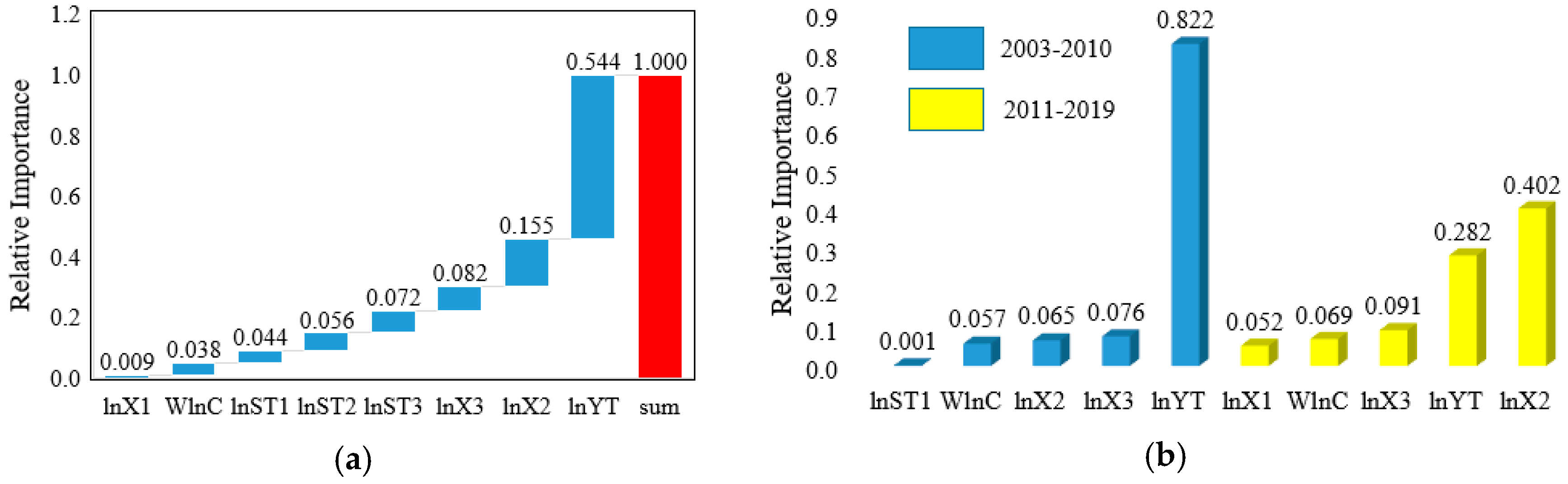
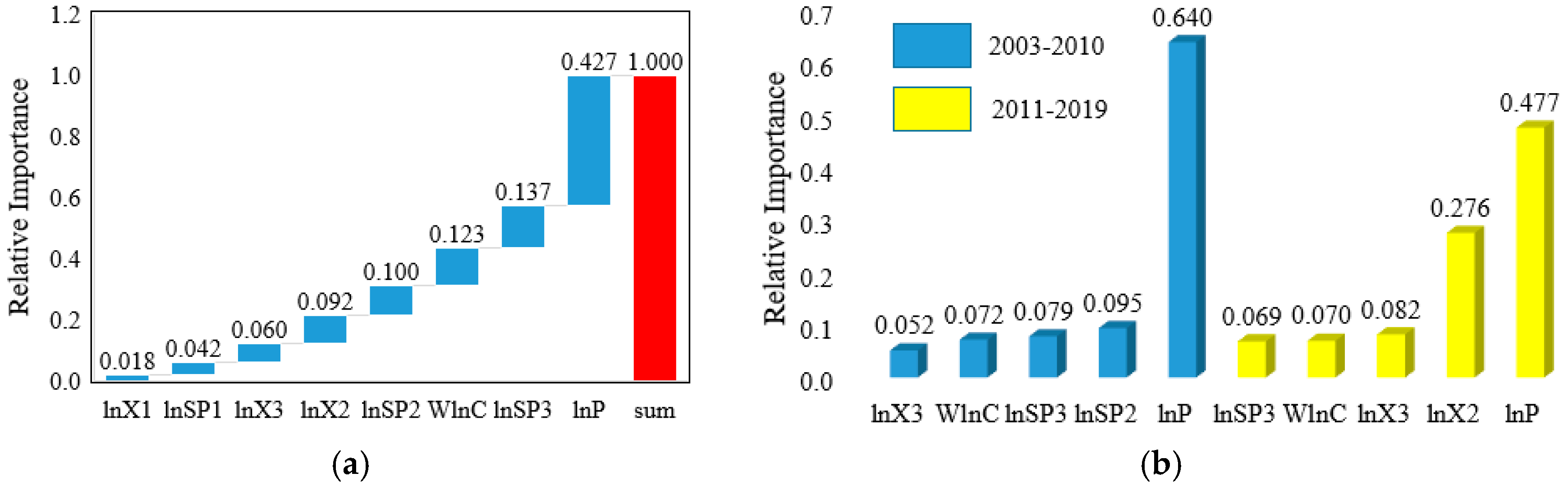
5. Relative Importance Analysis of Influencing Factors of CO2 Emissions in the Power Industry

The SDM can explore significant influencing factors of CO2 emissions in China’s power industry. However, it cannot demonstrate which factors are the key driving forces. Therefore, relative importance (RI) analysis was used to study the relative contributions of significant factors based on the SDM.

5.1. RI Analysis

RI analysis is used to compare the relative contribution of different independent variables to the dependent variable based on regression models. RI analysis is widely used in management, psychology and sociology. For example, Kantakumar et al. applied RI analysis to study the driving factors of urban growth in Pune [33]. Tang and He used RI analysis to explore the influence factors of total energy efficiency of the Yangtze River Economic Belt based on a panel model [34]. This paper chose the RI method of Ye et al. to discuss the main driving factors of CO2 emissions in the power industry [35].
For explaining the RI method better, a linear model is shown in Equation (9).
y = α + β 1 x 1 + β 2 x 2 + ε
For studying the contribution of x2 to y, two subset models were considered, as shown in Equations (10) and (11).
The   subset   model   1 :   y = α + β 2 x 2 + ε
The   subset   model   2 :   y = α + β 1 x 1 + ε
where R I 1 = R 2 ( x 2 ) represents the contribution of x 2 in subset model 1. The contribution of x2 can also be estimated as R I 2 = R 2 ( x 1 , x 2 ) R 2 ( x 1 ) based on the based model and subset model 2. Then, the contribution of x2 can be used as R I = ( R I 1 + R I 2 ) / 2 .
However, according to the SDM setting, there are eight independent variables in the based model, which can be written as Equation (12).
ln C i t = ρ W ln C t + r = 1 3 β 1 r ln X r , i t + j = 1 2 β 2 j ln S j , i t + β 3 ln Y i t + μ i + ε i t
There are also nine independent variables in each sector model, which can be written as Equation (13).
ln C i t = ρ W ln C i t + r = 1 3 β 1 r ln X r , i t + j = 1 3 β 2 j ln S X j , i m t + β 3 ln Y X i t m + μ i + ε i t
We needed to construct 2 8 1 subset models in the based model and 2 9 1 subset models in each sector model. We used Stata software to carry out RI analysis.

5.2. Results of RI Analysis

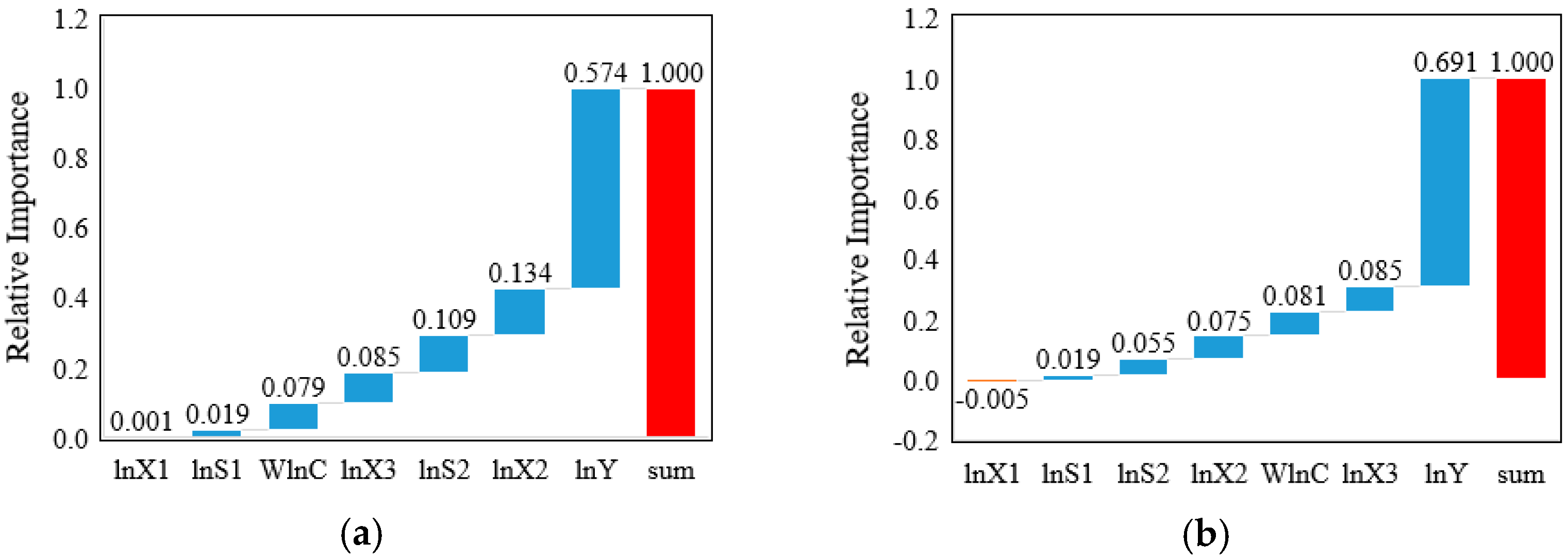
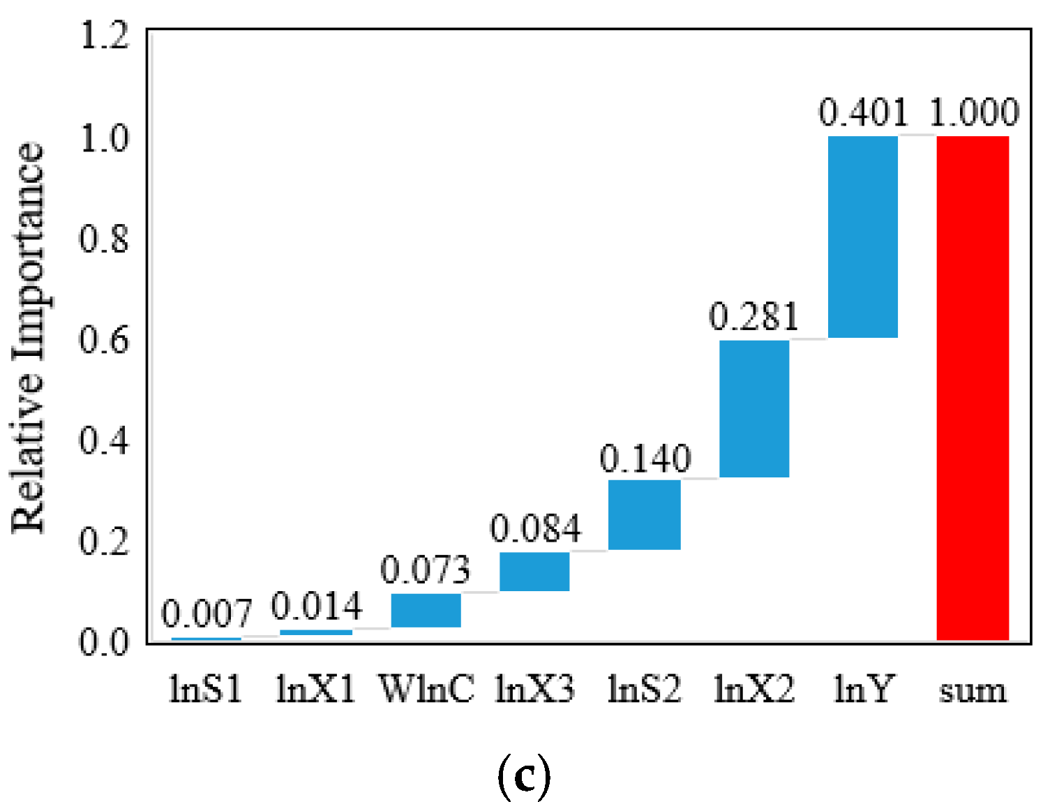
5.2.1. RI Analysis of the Based Model

Figure 1 shows the RI analysis of the based model. From 2003 to 2019, factors of CO2 emissions in China’s power industry can be ordered based on the RI analysis, as shown in Equation (14).
ln Y > ln X 2 > ln S 2 > ln X 3 > W ln C > ln S 1 > ln X 1
GDP is the most important factor for CO2 emissions in the power industry, followed by the power supply structure and energy intensity. Our conclusions are similar to those of He et al. [36] and Liao et al. [37], who used the LMDI method. The relative importance of ln Y between 2011 and 2019 decreased by 0.29 compared with that between 2003 and 2010. The relative importance of ln X 2 and ln S 2 increased by 0.166 and 0.065, respectively. On the one hand, the concept of “sustainable development” has been popular in China since 2011. Renewable power generation was accelerated by government subsidies [38]. Governments also shut down a large amount of outdated thermal power capacity. On the other hand, China’s energy intensity has continued to decline since 2011. It dropped by 14% during the 13th Five-Year Plan period. Because renewable energy and energy-saving technology are developing rapidly, the marginal contribution of economic development to CO2 emissions in the power industry is getting increasingly smaller. China’s economic development has been shifting to low-carbon development.
The self-supply ratio of electricity and the spatial spillover effect make a small positive contribution to CO2 emissions in the power industry. The relative importance of ln X 3 and W ln C between 2011 and 2019 was smaller than that between 2003 and 2010. Increasing power outsourcing can reduce the total CO2 emissions in the local power industry through inter-provincial energy trade. However, inter-provincial energy trade has little effect on the reduction in CO2 emissions in the local power industry due to inter-provincial trade barriers, such as local protectionism [39] and infrastructure differences [40].
ln S 1 and ln X 1 had the lowest relative importance in all periods. This shows that the energy demand structure and carbon emission intensity of thermal power make little contribution to CO2 emissions in the power industry. First, thermal power generating units have a design life of 30 years generally, so the relevant equipment and technology update slowly. Second, China’s thermal power efficiency has reached a high level, meaning that there is little room for improvement. Therefore, the relative importance of the CO2 emission intensity of thermal power is small. The proportion of electricity in energy consumption in 2019 increased by only 0.074 compared with that in 2003. The slow rate of electrification indicates there are few CO2 emissions transferred from consumption to the power industry.
In summary, it is more important for the low-carbon transformation of the power industry to promote renewable power and inter-provincial power trade than to improve thermal power efficiency. On the demand side, the importance of energy-saving technology progress is significantly greater than that of electrification.

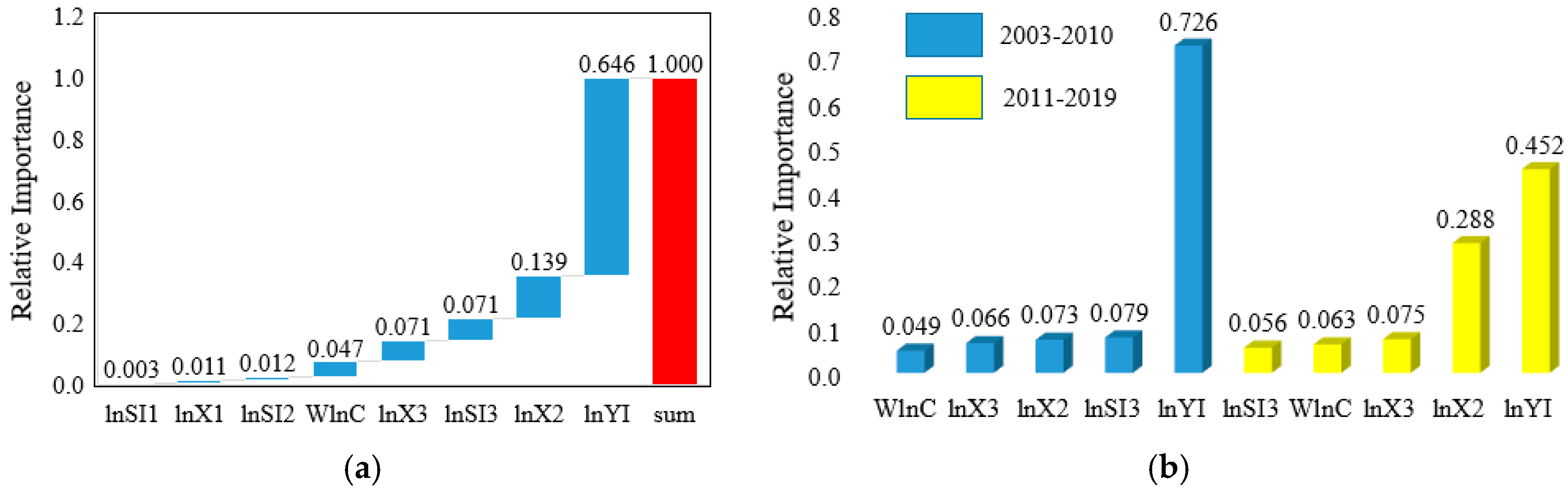
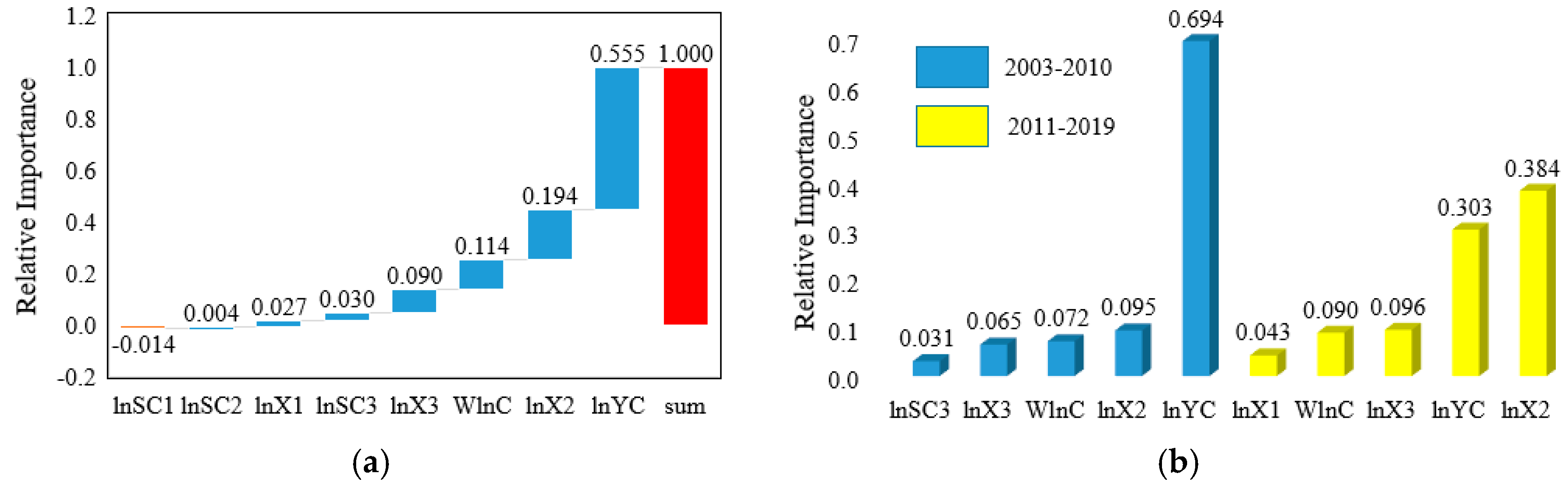
5.2.2. RI Analysis of Sector Models

The RI analysis results of the sector models are shown in Figure 2, Figure 3, Figure 4 and Figure 5. ln Y I , ln Y C , ln Y T and ln P had a larger relative importance between 2003 and 2019. This also indicates that the expansion of the sector scale is the main driving force for the increase in CO2 emissions in the power industry. The contributions of the four sector sizes between 2011 and 2019 decreased by 0.274, 0.391, 0.540 and 0.163 compared with those between 2003 and 2010, respectively. The marginal contribution of the sector size to the CO2 emissions in the power industry is getting increasingly smaller. The conclusion is the same as that of the based model and can be credible. The scale contribution of the transport and construction sectors declined faster than that of the industry and resident sectors. Their scale contribution was even below the contribution of the power supply structure between 2011 and 2019. This shows that CO2 emissions in the power industry are mainly caused by the energy demand of the industrial sector and the residential sector at present.
The relative importance of ln S I 3 was larger than that of ln S I 2 in all periods. Compared with electrification, the improvement of energy-saving technology in the industrial sector has a greater impact on the CO2 emissions in the power industry. Energy intensity in all provinces dropped significantly from 2003 to 2019. The progress of energy-saving technology in the industrial sector has reduced the total power demand effectively. The progress of energy-saving technology has played a positive role in promoting the reduction in CO2 emissions in the power industry. However, the contribution of energy-saving technology progress is decreasing, because it is getting harder to improve energy efficiency in the industrial sector.
The relative importance of ln S P 3 was larger than that of ln S P 2 between 2003 and 2019. This indicates that the contribution of per capita energy consumption to CO2 emissions in the power industry is greater than that of electrification. However, ln S P 3 had less relative importance than ln S P 2 between 2003 and 2010. With income increasing, people have an increasing demand for energy consumption. They prefer cleaner and more convenient electricity [41]. As a result, the residential sector has transferred a large amount of CO2 emissions to the power industry. At present, the growth of per capita energy consumption demand is still fast in China. The residential sector will put more pressure on CO2 emissions in the power industry.
In summary, the industry and residential sectors contribute more to CO2 emissions in the power industry than construction and transportation. The contribution of energy-saving technology to CO2 emissions is also greater than that of electrification in each sector. Therefore, it is of great importance for the low-carbon transformation of the power industry to give priority to promoting the progress of the industry’s energy-saving technology and the green living concept.

6. Conclusions

The low-carbon transformation of the power industry is of great significance to realize the “carbon peak” in advance. For exploring the main driving factors, the Kaya equation was used to decompose the CO2 emissions in the power industry into seven factors. These factors included the carbon emission intensity of thermal power, power supply structure, self-supply ratio of electricity, energy demand structure, energy intensity and GDP. Then, the spatial Durbin model and relative importance analysis were constructed based on the provincial data of China from 2003 to 2019. Based on the relative importance, these factors can be ranked in the order GDP, power supply structure, energy intensity, self-supply ratio of electricity, spatial spillover effect, energy demand structure and CO2 emission intensity of thermal power. GDP is the main driver of carbon emissions from China’s power sector. Economic development was responsible for almost 60% of CO2 emissions in China’s power industry between 2003 and 2019. With China’s low-carbon development, economic development has increasingly less impact on CO2 emissions in the power industry. The relative importance of the power supply structure and energy intensity increased between 2003 and 2019. This indicates that renewable energy power development and energy-saving technology progress are becoming increasingly important for the low-carbon development of the power industry. The self-supply ratio and spatial spillover effect make a positive contribution to CO2 emissions in the local power industry, but their contributions are very small. This shows that the expansion of inter-regional power trade will not promote the CO2 emissions in the regional power industry significantly. In the sector analysis, the impact of energy-saving technology progress was greater than that of electrification on CO2 emissions in the power industry. It is necessary to promote energy-saving technology progress in the demand sectors. This also shows that the sector size of industry and residents has a greater impact than that of construction and transportation on the CO2 emissions in the power industry.
With high-quality economic development, there will be increasing pressure on the CO2 emission reduction in the power industry. Based on the conclusions, three policy suggestions are put forward to promote the low-carbon transformation of the power industry. First, on the power supply side, the main strategy is the low-carbon transformation of the power supply structure. The auxiliary strategy is to reduce the carbon emission intensity of thermal power. Governments should make more efforts to develop renewable power and reduce outdated coal-fired power as opposed to improving the efficiency of thermal power generation. Second, based on the premise of regional CO2 emission equity, regional electricity trade should be encouraged to promote the rapid development of the power industry. Third, on the energy demand side, governments should make energy-saving technology innovation as the main strategy and electrification as the auxiliary strategy. The energy saving potential of the industry and resident sectors should be tapped deeply to reduce the regional power demand in particular. These suggestions will lead to increasingly less impact of economic development on the CO2 emissions in the power industry.

Author Contributions

Conceptualization, W.Z. and Y.C.; methodology, W.Z. and Y.H.; software, W.Z.; validation, W.Z., Y.C. and S.T.; formal analysis, W.Z.; investigation, W.Z.; resources, W.Z.; data curation, W.Z. and Y.H.; writing—original draft preparation, W.Z.; writing—review and editing, W.Z. and S.T.; visualization, Y.C.; supervision, Y.C. and S.T.; project administration, Y.C.; funding acquisition, Y.C. All authors have read and agreed to the published version of the manuscript.

Funding

This paper was supported by the Humanities and Social Sciences Planning Fund Project of the Ministry of Education (21YJA790009). The funder is Yuanying Chi.

Institutional Review Board Statement

This study did not involve humans or animals.

Informed Consent Statement

Not applicable.

Data Availability Statement

The analysis data were taken from the China Statistical Yearbook, the China Energy Statistical Yearbook and the Carbon Emission Accounts and Datasets.

Conflicts of Interest

The authors declare no conflict of interest.

References

  1. BP. BP Statistical Review of World Energy 2021, 70th ed.; BP: London, UK, 2021. [Google Scholar]
  2. Li, W.; Zhang, Y.; Lu, C. The impact on electric power industry under the implementation of national carbon trading market in China: A dynamic CGE analysis. J. Clean. Prod. 2018, 200, 511–523. [Google Scholar] [CrossRef]
  3. Xie, P.; Yang, F.; Mu, Z.; Gao, S. Influencing factors of the decoupling relationship between CO2 emission and economic development in China’s power industry. Energy (Oxford) 2020, 209, 118341. [Google Scholar] [CrossRef]
  4. Jia, Z.; Lin, B. The impact of removing cross subsidies in electric power industry in China: Welfare, economy, and CO2 emission. Energy Policy 2021, 148, 111994. [Google Scholar] [CrossRef]
  5. Wu, H.; Xu, L.; Ren, S.; Hao, Y.; Yan, G. How do energy consumption and environmental regulation affect carbon emissions in China? New evidence from a dynamic threshold panel model. Resour. Policy 2020, 67, 101678. [Google Scholar]
  6. Tang, B.; Li, R.; Yu, B.; An, R.; Wei, Y. How to peak carbon emissions in China’s power sector: A regional perspective. Energy Policy 2018, 120, 365–381. [Google Scholar] [CrossRef]
  7. Li, J.; Zhang, Y.; Tian, Y.; Cheng, W.; Yang, J.; Xu, D.; Wang, Y.; Xie, K.; Ku, A.Y. Reduction of carbon emissions from China’s coal-fired power industry: Insights from the province-level data. J. Clean. Prod. 2020, 242, 118518. [Google Scholar] [CrossRef]
  8. Zhang, L.; Du, Q.; Zhou, D.; Zhou, P. How does the photovoltaic industry contribute to China’s carbon neutrality goal? Analysis of a system dynamics simulation. Sci. Total Environ. 2022, 808, 151868. [Google Scholar]
  9. Lin, B.; Bega, F. China’s Belt & Road Initiative coal power cooperation: Transitioning toward low-carbon development. Energy Policy 2021, 156, 112438. [Google Scholar]
  10. Yu, Y.; Jin, Z.; Li, J.; Jia, L. Low-carbon development path research on China’s power industry based on synergistic emission reduction between CO2 and air pollutants. J. Clean. Prod. 2020, 275, 123097. [Google Scholar] [CrossRef]
  11. Yang, L.; Lin, B. Carbon dioxide-emission in China’s power industry: Evidence and policy implications. Renew. Sustain. Energy Rev. 2016, 60, 258–267. [Google Scholar] [CrossRef]
  12. Cui, H.; Zhao, T.; Wu, R. CO2 emissions from China’s power industry: Policy implications from both macro and micro perspectives. J. Clean. Prod. 2018, 200, 746–755. [Google Scholar] [CrossRef]
  13. Ling, Y.; Xia, S.; Cao, M.; He, K.; Lim, M.K.; Sukumar, A.; Yi, H.; Qian, X. Carbon emissions in China’s thermal electricity and heating industry: An input-output structural decomposition analysis. J. Clean. Prod. 2021, 329, 129608. [Google Scholar] [CrossRef]
  14. Jiang, T.; Yang, J.; Huang, S. Evolution and driving factors of CO2 emissions structure in China’s heating and power industries: The supply-side and demand-side dual perspectives. J. Clean. Prod. 2020, 264, 121507. [Google Scholar] [CrossRef]
  15. Quan, C.; Cheng, X.; Yu, S.; Ye, X. Analysis on the influencing factors of carbon emission in China’s logistics industry based on LMDI method. Sci. Total Environ. 2020, 734, 138473. [Google Scholar] [CrossRef] [PubMed]
  16. Liu, X.; Peng, R.; Zhong, C.; Wang, M.; Guo, P. What drives the temporal and spatial differences of CO2 emissions in the transport sector? Empirical evidence from municipalities in China. Energy Policy 2021, 159, 112607. [Google Scholar] [CrossRef]
  17. Tang, Z.; Yu, H.; Zou, J. How does production substitution affect China’s embodied carbon emissions in exports? Renew. Sustain. Energy Rev. 2022, 156, 111957. [Google Scholar] [CrossRef]
  18. Ninpanit, P.; Malik, A.; Wakiyama, T.; Geschke, A.; Lenzen, M. Thailand’s energy-related carbon dioxide emissions from production-based and consumption-based perspectives. Energy Policy 2019, 133, 110877. [Google Scholar] [CrossRef]
  19. Cai, W.; Song, X.; Zhang, P.; Xin, Z.; Zhou, Y.; Wang, Y.; Wei, W. Carbon emissions and driving forces of an island economy: A case study of Chongming Island, China. J. Clean. Prod. 2020, 254, 120028. [Google Scholar] [CrossRef]
  20. Zhao, P.; Zeng, L.; Li, P.; Lu, H.; Hu, H.; Li, C.; Zheng, M.; Li, H.; Yu, Z.; Yuan, D.; et al. China’s transportation sector carbon dioxide emissions efficiency and its influencing factors based on the EBM DEA model with undesirable outputs and spatial Durbin model. Energy 2022, 238, 121934. [Google Scholar] [CrossRef]
  21. Li, J.; Li, S. Energy investment, economic growth and carbon emissions in China—Empirical analysis based on spatial Durbin model. Energy Policy 2020, 140, 111425. [Google Scholar] [CrossRef]
  22. Espoir, D.K.; Sunge, R. CO2 emissions and economic development in Africa: Evidence from a dynamic spatial panel model. J. Environ. Manag. 2021, 300, 113617. [Google Scholar] [CrossRef] [PubMed]
  23. Croonenbroeck, C.; Palm, M. A spatio-temporal Durbin fixed effects IV-Model for ENTSO-E electricity flows analysis. Renew. Energy 2020, 148, 205–213. [Google Scholar] [CrossRef]
  24. Park, J.; Yun, S. Social determinants of residential electricity consumption in Korea: Findings from a spatial panel model. Energy (Oxford) 2022, 239, 122272. [Google Scholar] [CrossRef]
  25. Yan, D.; Lei, Y.; Li, L.; Song, W. Carbon emission efficiency and spatial clustering analyses in China’s thermal power industry: Evidence from the provincial level. J. Clean. Prod. 2017, 156, 518–527. [Google Scholar] [CrossRef]
  26. Wang, Z.; Zhu, H.; Ding, Y.; Zhu, T.; Zhu, N.; Tian, Z. Energy efficiency evaluation of key energy consumption sectors in China based on a macro-evaluating system. Energy 2018, 153, 65–79. [Google Scholar] [CrossRef]
  27. Chen, Y.; Lee, C. Does technological innovation reduce CO2 emissions? Cross-country evidence. J. Clean. Prod. 2020, 263, 121550. [Google Scholar] [CrossRef]
  28. Lv, Y.; Chen, W.; Cheng, J. Modelling dynamic impacts of urbanization on disaggregated energy consumption in China: A spatial Durbin modelling and decomposition approach. Energy Policy 2019, 133, 110841. [Google Scholar] [CrossRef]
  29. Zhao, J.; Jiang, Q.; Dong, X.; Dong, K.; Jiang, H. How does industrial structure adjustment reduce CO2 emissions? Spatial and mediation effects analysis for China. Energy Econ. 2022, 105, 105704. [Google Scholar]
  30. Zhang, L.; Li, R. Impacts of green certification programs on energy consumption and GHG emissions in buildings: A spatial regression approach. Energy Build. 2022, 256, 111677. [Google Scholar] [CrossRef]
  31. Tan, Z.; Li, L.; Wang, J.; Wang, J. Examining the driving forces for improving China’s CO2 emission intensity using the decomposing method. Appl. Energy 2011, 88, 4496–4504. [Google Scholar] [CrossRef]
  32. Liao, C.; Wang, S.; Zhang, Y.; Song, D.; Zhang, C. Driving forces and clustering analysis of provincial-level CO2 emissions from the power sector in China from 2005 to 2015. J. Clean. Prod. 2019, 240, 118026. [Google Scholar] [CrossRef]
  33. Kantakumar, L.N.; Kumar, S.; Schneider, K. What drives urban growth in Pune? A logistic regression and relative importance analysis perspective. Sustain. Cities Soc. 2020, 60, 102269. [Google Scholar]
  34. Tang, L.; He, G. How to improve total factor energy efficiency? An empirical analysis of the Yangtze River economic belt of China. Energy 2021, 235, 121375. [Google Scholar]
  35. Ye, D.; Ng, Y.; Lian, Y. Culture and Happiness. Soc. Indic. Res. 2015, 123, 519–547. [Google Scholar] [CrossRef] [Green Version]
  36. He, Y.; Xing, Y.; Zeng, X.; Ji, Y.; Hou, H.; Zhang, Y.; Zhu, Z. Factors influencing carbon emissions from China’s electricity industry: Analysis using the combination of LMDI and K-means clustering. Environ. Impact Assess. 2022, 93, 106724. [Google Scholar] [CrossRef]
  37. Liao, C.; Wang, S.; Fang, J.; Zheng, H.; Liu, J.; Zhang, Y. Driving forces of provincial-level CO2 emissions in China’s power sector based on LMDI method. Energy Procedia 2019, 158, 3859–3864. [Google Scholar] [CrossRef]
  38. Tang, S.; Zhou, W.; Li, X.; Chen, Y.; Zhang, Q.; Zhang, X. Subsidy strategy for distributed photovoltaics: A combined view of cost change and economic development. Energy Econ. 2021, 97, 105087. [Google Scholar] [CrossRef]
  39. Zhu, X.; He, C.; Gu, Z. How do local policies and trade barriers reshape the export of Chinese photovoltaic products? J. Clean. Prod. 2021, 278, 123995. [Google Scholar] [CrossRef]
  40. Xu, J.; Yi, B.; Fan, Y. Economic viability and regulation effects of infrastructure investments for inter-regional electricity transmission and trade in China. Energy Econ. 2020, 91, 104890. [Google Scholar] [CrossRef]
  41. Pellini, E. Estimating income and price elasticities of residential electricity demand with Autometrics. Energy Econ. 2021, 101, 105411. [Google Scholar] [CrossRef]
Figure 1. RI analysis of the based model in different periods. (a) RI analysis between 2003 and 2019; (b) RI analysis between 2003 and 2010; (c) RI analysis between 2011 and 2019.
Energies 15 02631 g001aEnergies 15 02631 g001b
Figure 2. RI analysis of the industry sector. (a) RI analysis between 2003 and 2019; (b) RI analysis in different periods. Note: For a better analysis, this paper only shows the top 5 factors that have a larger relative importance in (b). In (b), blue represents 2003–2010, and yellow represents 2011–2019.
Energies 15 02631 g002
Figure 3. RI analysis of the construction sector. (a) RI analysis between 2003 and 2019; (b) RI analysis in different periods. Note: For a better analysis, this paper only shows the top 5 factors that have a larger relative importance in (b). In (b), blue represents 2003–2010, and yellow represents 2011–2019.
Energies 15 02631 g003
Figure 4. RI analysis of the transportation sector. (a) RI analysis between 2003 and 2019; (b) RI analysis in different periods. Note: For a better analysis, this paper only shows the top 5 factors that have a larger relative importance in (b). In (b), blue represents 2003–2010, and yellow represents 2011–2019.
Energies 15 02631 g004
Figure 5. RI analysis of the resident sector. (a) RI analysis between 2003 and 2019; (b) RI analysis in different periods. Note: For a better analysis, this paper only shows the top 5 factors that have a larger relative importance in (b). In (b), blue represents 2003–2010, and yellow represents 2011–2019.
Energies 15 02631 g005
Table 1. Definitions and descriptive statistics for all variables.
TypeVariableVariable DefinitionFormulaMeanStdMinMaxMedian
Based model ln C CO2 emissions ln C = ln ( C ) 4.56800.89411.84226.40384.6026
ln X 1 CO2 emission intensity of thermal power ln X 1 = ln ( C / S × 100 ) 2.50150.21801.96733.22862.4744
ln X 2 Power supply structure ln X 2 = ln ( S / E S × 100 ) 4.26050.45522.09314.60514.4278
ln X 3 Self-supply ratio of electricity ln X 3 = ln ( E S / E C × 100 ) 4.60550.29903.46585.26284.6051
ln S 1 Energy demand structure ln S 1 = ln ( E C / T C × 100 ) 3.24020.27850.49113.97073.2255
ln S 2 Energy intensity ln S 2 = ln ( T C / Y × 100 ) 4.28360.55462.80146.21084.3065
ln Y GDP ln Y = ln ( Y ) 9.23741.06495.953211.58989.3536
Industry model ln S X 1 Proportion of industrial power consumption ln S I 1 = ln ( E C I / E C × 100 + 1 ) 4.07430.25112.72884.49544.1061
ln S X 2 Industrial energy demand structure ln S I 2 = ln ( E C I / T C I × 100 + 1 ) 3.31340.36230.48014.24873.2551
ln S X 3 Industrial energy intensity ln S I 3 = ln ( T C I / Y I × 100 + 1 ) 4.69790.64592.87976.72624.7563
ln Y X Industrial added value ln Y I = ln ( Y I ) 8.18931.15504.369410.57498.2675
Construction model ln S X 1 Proportion of construction’s power consumption ln S C 1 = ln ( E C C / E C × 100 + 1 ) 0.72340.272901.82640.6750
ln S X 2 Construction’s energy demand structure ln S C 2 = ln ( E C C / T C C × 100 + 1 ) 2.97450.591604.49283.0118
ln S X 3 Construction’s energy intensity ln S C 3 = ln ( T C C / Y C × 100 + 1 ) 2.72410.63511.02716.50792.7680
ln Y X Added value in construction ln Y C = ln ( Y C ) 6.52851.03283.72818.75316.5476
Transportation model ln S X 1 Proportion of transportation’s power consumption ln S T 1 = ln ( E C T / E C × 100 + 1 ) 1.01640.35330.29762.24890.9647
ln S X 2 Transportation’s energy demand structure ln S T 2 = ln ( E C T / T C T × 100 + 1 ) 1.70330.51180.09653.20811.6483
ln S X 3 Transportation’s energy intensity ln S T 3 = ln ( T C T / Y T × 100 + 1 ) 4.85440.43453.63885.80434.8721
ln Y X Added value in transportation ln Y T = ln ( Y T ) 6.29430.94163.22288.20476.3846
Resident model ln S X 1 Proportion of residents’ power consumption ln S P 1 = ln ( E C P / E C × 100 + 1 ) 2.73240.42250.19723.83922.7492
ln S X 2 Residents’ energy demand structure ln S P 2 = ln ( E C P / T C P × 100 + 1 ) 3.56720.45580.06814.30673.6043
ln S X 3 Per capita energy consumption ln S P 3 = ln ( T C P / P × 100 + 1 ) 3.09900.53921.29254.33213.1294
ln Y X Population ln P = ln ( P ) 8.17350.75226.28049.43268.2506
Table 2. Unit root tests.
VariableLLC TestIPS TestFisher TestConclusionVariableLLC TestIPS TestFisher TestConclusion
ln C −3.30 ***−3.49 ***165.20 ***Stationary ln S C 2 −10.84 ***−2.80 ***155.20 ***Stationary
ln X 1 −4.20 ***−2.95 ***118.86 ***Stationary ln S C 3 −14.36 ***−3.23 ***145.13 ***Stationary
ln X 2 −2.67 ***−4.33 ***96.85 ***Stationary ln Y C −1.49 *−4.89 ***242.27 ***Stationary
ln X 3 −2.75 ***−4.59 ***151.41 ***Stationary ln S T 1 −8.15 ***−2.99 ***111.09 ***Stationary
ln S 1 −5.17 ***−4.63 ***101.90 ***Stationary ln S T 2 −6.77 ***−3.56 ***123.10 ***Stationary
ln S 2 −2.06 **−2.25 **105.38 ***Stationary ln S T 3 −4.74 ***−4.06 ***149.72 ***Stationary
ln Y −2.94 ***−4.84 ***248.95 ***Stationary ln Y T −4.29 ***−3.64 ***164.47 ***Stationary
ln S I 1 −5.75 ***−1.37 *119.88 ***Stationary ln S P 1 −4.54 ***−4.40 ***151.38 ***Stationary
ln S I 2 −14.27 ***−4.38 ***152.56 ***Stationary ln S P 2 −14.19 ***−3.54 ***163.20 ***Stationary
ln S I 3 −3.19 ***−4.75 ***144.14 ***Stationary ln S P 3 −11.69 ***−3.63 ***145.82 ***Stationary
ln Y I −4.58 ***−6.77 ***246.85 ***Stationary ln P −2.51 ***0.63136.47 ***Stationary
ln S C 1 −5.29 ***−3.18 ***133.51 ***Stationary
Note: *, ** and *** indicate statistical significance at 10%, 5% and 1%, respectively.
Table 3. Geary’s C index of CO2 emissions in the power industry.
Year200320042005200620072008200920102011
Geary’s C0.760 **
(−2.33)
0.778 **
(−2.168)
0.793 **
(−1.992)
0.807 **
(−1.860)
0.817 **
(−1.764)
0.798 **
(−1.954)
0.798 **
(−1.958)
0.807 **
(−1.846)
0.835 *
(−1.589)
Year20122013201420152016201720182019
Geary’s C0.834 *
(−1.608)
0.826 **
(−1.688)
0.821 **
(−1.754)
0.803 **
(−1.951)
0.790 **
(−2.098)
0.802 **
(−1.986)
0.815 **
(−1.834)
0.827 **
(−1.705)
Note: * and ** indicate statistical significance at 10% and 5%, respectively. The values in parentheses represent z statistics.
Table 4. Results of five regressions.
VariableOLSPMSARSEMSDM
ln X 1 0.2853 ***
(6.26)
0.7277 ***
(3.86)
0.7218 ***
(14.08)
0.7084 ***
(13.96)
0.6974 ***
(13.83)
ln X 2 0.8214 ***
(39.59)
0.9921 ***
(14.21)
0.9828 ***
(27.55)
0.9941 ***
(28.51)
1.0209 ***
(28.40)
ln X 3 1.0312 ***
(31.03)
1.0374 ***
(7.85)
1.0304 ***
(17.50)
1.0274 ***
(17.59)
1.0382 ***
(17.45)
ln S 1 0.4728 ***
(14.89)
0.1463
(0.88)
0.1451 ***
(5.08)
0.1345 ***
(4.82)
0.1432 ***
(5.12)
ln S 2 0.9594 ***
(34.36)
0.6241 ***
(2.99)
0.6126 ***
(14.34)
0.6494 ***
(15.43)
0.6415 ***
(15.20)
ln Y 0.9722 ***
(78.57)
0.9082 ***
(10.13)
0.8768 ***
(27.46)
0.9281 ***
(40.96)
0.8045 ***
(11.06)
ρ 0.0616
(1.30)
0.2812 ***
(3.67)
0.2460 **
(3.84)
σ 0.0105 ***
(15.97)
0.0102 ***
(15.84)
0.0100 ***
(15.90)
R 2 0.95910.92880.92520.92320.9211
Note: The table does not show constant terms or interaction terms of the inverse distance matrix and explanatory variables. ** and *** indicate statistical significance at 5% and 1%, respectively. The values in parentheses represent z statistics.
Table 5. Regression results of sector models.
VariableIndustryConstructionTransportationResidents
ln X 1 0.6451 ***
(12.78)
0.8457 ***
(15.69)
0.8892 ***
(18.65)
0.8254 ***
(16.42)
ln X 2 0.9976 ***
(27.46)
1.0146 ***
(24.19)
1.0420 ***
(27.41)
1.0313 ***
(25.95)
ln X 3 1.0015 ***
(16.31)
0.9984 ***
(14.38)
1.0359 ***
(16.16)
1.0549 ***
(15.52)
ln S X 1 −0.0227
(−0.39)
−0.3050 ***
(−6.70)
−0.5271 ***
(−12.68)
−0.4298 ***
(−12.26)
ln S X 2 0.1521 ***
(6.68)
0.1443 ***
(7.27)
0.3281 ***
(11.16)
0.2770 ***
(11.48)
ln S X 3 0.4071 ***
(12.38)
0.1809 ***
(7.99)
0.2658 ***
(8.20)
0.3553 ***
(11.37)
ln Y X 0.3853 ***
(9.58)
0.3695 ***
(9.11)
0.4452 ***
(9.77)
0.4347 ***
(3.90)
ρ 0.2936 ***
(4.02)
0.2203 ***
(3.57)
0.0911 *
(1.74)
0.4655 ***
(8.26)
σ 0.0106 ***
(15.84)
0.0135 ***
(15.92)
0.0114 ***
(15.96)
0.0122 ***
(15.72)
R 2 0.77730.75650.79870.8228
Note: The table does not show constant terms or interaction terms of the inverse distance matrix and explanatory variables. * and *** indicate statistical significance at 10% and 1%, respectively. The values in parentheses represent z statistics.
Publisher’s Note: MDPI stays neutral with regard to jurisdictional claims in published maps and institutional affiliations.

